import os

for v_ in ("OMP_NUM_THREADS", "OPENBLAS_NUM_THREADS", "MKL_NUM_THREADS"):
    os.environ[v_] = "1"  # nutpie runs chains as threads: a BLAS pool per chain would fight over the cores

import itertools
import logging
import sys
import time
import warnings

import arviz as az
import matplotlib.pyplot as plt
import numpy as np
import pandas as pd
import pymc as pm
from scipy import special, stats

from pymc_challenges import data

RANDOM_SEED = 101
rng = np.random.default_rng(RANDOM_SEED)
az.style.use("arviz-variat")
logging.getLogger("pymc").setLevel(logging.WARNING)
warnings.filterwarnings("ignore", category=FutureWarning)
warnings.filterwarnings("ignore", category=UserWarning, module="arviz")
sys.modules.pop("jax", None)  # arviz leaves a lazy jax stub that makes matplotlib import all of JAX
pd.set_option("display.width", 160)
T_START = time.time()

BLUE, ORANGE, AQUA, PURPLE, RED = "#2a78d6", "#eb6834", "#1baf7a", "#8c5ac8", "#c8384e"
INK, MUTED, LIGHT = "#222222", "#8a8984", "#d9d8d3"
KPIS = ["visit", "conversion"]
print(f"PyMC {pm.__version__}, ArviZ {az.__version__}")
PyMC 6.3.2, ArviZ 1.3.0
The setting
A brand manager has just run a campaign and asks the question every campaign ends with: did the ads work, and by how much? The usual tool is a brand lift study. A survey vendor recruits people who saw the ads and people who did not, asks both groups the same questions (do you know the brand, would you consider it, do you intend to buy), and reports the difference as the campaign's lift. Done well, the "did not see the ads" group is a randomised holdout: people the platform deliberately kept away from the campaign. Done the cheap way, it is everyone else - people who simply happened not to be reached - and the vendor tries to make the two groups comparable after the fact, by matching or weighting on what it knows about the respondents.
That after-the-fact correction is propensity score analysis (Rosenbaum & Rubin 1983): model each person's probability of being exposed from their characteristics, then compare exposed and unexposed people who had the same probability. If everything that drives both exposure and the outcome is among the characteristics, the comparison is as good as an experiment. Advertising is a hard place for that "if". Ad platforms deliver ads to the people most likely to respond - active users, people who recently visited the advertiser's site, people already in the market - so exposure is tangled up with intent. Gordon, Zettelmeyer, Bhargava & Chapsky (2019) tested this directly on 15 large Facebook campaigns that had been run as randomised experiments: they reran each one as an observational study with Facebook's rich user data, and the propensity-based methods often overstated the lift, in some campaigns several times over. Lewis & Rao (2015) explained why ad effects are so hard to measure at all: the effect of one campaign on one person is tiny next to the noise in their behaviour.
This notebook repeats that test on public data. No respondent-level brand lift survey is public, so we use the closest real thing: Criteo's uplift dataset (Diemert et al. 2018), assembled from randomised incrementality tests. Each user was assigned at random to a test arm, where the campaign could show them ads, or a control arm, where it could not; the file records whether each test user was actually shown an ad, and what they did over the next two weeks. That gives us both halves of the comparison in one data set: the observational "exposed versus unexposed" study a vendor would run, and the randomised experiment that grades it. The brand KPI is a stand-in. Criteo records a visit to the advertiser's site and a conversion, not a survey answer. We use the visit as the upper-funnel KPI (it is what consideration surveys try to measure: did the person engage with the brand) and the conversion as the lower-funnel one, and we treat each user as a respondent. Nothing in the statistics depends on how the outcome was collected; what matters is that the people who saw the ads differ from those who did not in ways that also drive the outcome.
C09 asked the same question of a job-training programme with LaLonde's data, and E63 used instrumental variables for quasi-experiments; here the treatment is an ad, the experiment lives inside the same file, and we can also replay the study at the size of a real survey.
| part | question | tool |
|---|---|---|
| A | What is in the data? | three cells: control, test-unexposed, test-exposed; the naive comparison |
| B | What does the experiment say? | intent-to-treat, the Wald estimate as a Bayesian principal-strata model; a balance check of the randomisation; regression adjustment from sufficient statistics |
| C | Why is exposure not random? | standardised mean differences; who gets an ad |
| D | Can we model exposure? | a Bayesian propensity model on a respondent file that oversamples the exposed; prior predictive, calibration, overlap, balance |
| E | What do propensity methods say? | IPW, stratification, outcome regression, AIPW, with propagated uncertainty; one figure against the experiment |
| F | Why do they miss? | the imputed baseline; adding features; flexibility |
| G | How strong is the hidden confounder? | E-values; a bias parameter in PyMC |
| H | What happens at survey size? | replayed surveys of 2,000-60,000 respondents; coverage; ghost ads |
| I | What should the brand manager report? | the decision and the next study |
A · The data
data.describe("e101_criteo_uplift")
raw = np.load(data.path("e101_criteo_uplift"))
cells = ["control", "test, unexposed", "test, exposed"]
full = pd.DataFrame({"users": raw["cell_n"], "visits": raw["cell_visit"], "conversions": raw["cell_conversion"]},
                    index=cells)
full["visit rate"] = full.visits / full.users
full["conversion rate"] = full.conversions / full.users
print(f"\nall {int(raw['n_total']):,} users in the file:")
print(full.to_string(formatters={"users": "{:,}".format, "visits": "{:,}".format, "conversions": "{:,}".format,
                                 "visit rate": "{:.4f}".format, "conversion rate": "{:.5f}".format}))
n_test = full.users.iloc[1:].sum()
print(f"\ntest share {n_test / full.users.sum():.3f}; exposed share of the test arm {full.users.iloc[2] / n_test:.4f}")
for k in KPIS:
    r = full[f"{k} rate"]
    print(f"{k:10s}: exposed {r.iloc[2]:.4f} vs unexposed {r.iloc[1]:.4f} -> difference {r.iloc[2] - r.iloc[1]:+.4f}, "
          f"ratio {r.iloc[2] / r.iloc[1]:.1f}x")
e101_criteo_uplift: npz. A simple random sample of 300,000 of the 13,979,592 users in Criteo's pooled incrementality tests (randomised holdouts; several advertisers' tests sub-sampled to one treatment ratio): X (300000, 12) float32 anonymised features f0-f11 (float64 in the source), treatment (1 = test arm, randomised, ~85%), exposure (1 = the user was actually shown an ad; only possible in test), visit (visited the advertiser's site), conversion, row (row in the source). Plus EXACT full-data counts for the cells control / test-unexposed / test-exposed: cell_n, cell_visit, cell_conversion (3,), and per-cell feature sums cell_xsum, cell_xsq (3, 12); full-data sufficient statistics of a 91-column basis of the features' normal scores (1, r, r^2, pairwise products): basis_zz (arm, 91, 91), basis_zy (arm, outcome, 91), basis_cell_sum (3, 91); n_total, seed. Absolute rates are not the campaign's: Criteo down-sampled negatives non-uniformly.
  source: Criteo Uplift Prediction Dataset v2.1: Diemert, Betlei, Renaudin & Amini (2018), 'A Large Scale Benchmark for Uplift Modeling', AdKDD workshop at KDD 2018. Licence CC BY-NC-SA 4.0 (non-commercial, share-alike; this extract carries the same licence). Criteo's original link (http://go.criteo.net/criteo-research-uplift-v2.1.csv.gz) answered 404 in November 2026; the file came from Criteo's own Hugging Face repository (311,422,618 bytes, sha256 2716e1bf0fd157a93b5bf86924d9088419dfbac2022c6cd90030220634f616dc). DERIVED by tools/build_e101_data.py (seed 101): the url is the 300 MB source, not this file - keep the cached npz in data/ (md5 9d7dee707a79e8a09bac50fafd96a299).
  url:    https://huggingface.co/datasets/criteo/criteo-uplift/resolve/main/criteo-research-uplift-v2.1.csv.gz

all 13,979,592 users in the file:
                     users  visits conversions visit rate conversion rate
control          2,096,937  80,105       4,063     0.0382         0.00194
test, unexposed 11,454,443 399,314      13,680     0.0349         0.00119
test, exposed      428,212 177,510      23,031     0.4145         0.05378

test share 0.850; exposed share of the test arm 0.0360
visit     : exposed 0.4145 vs unexposed 0.0349 -> difference +0.3797, ratio 11.9x
conversion: exposed 0.0538 vs unexposed 0.0012 -> difference +0.0526, ratio 45.0x
The campaign file has three cells. 2.1 million users were held out in control; 11.9 million were in the test arm, of whom only 428,212 (3.6%) were actually shown an ad. The ad server reaches a user only when they show up somewhere it can bid; most test users never did. No control user was exposed. (The file pools several advertisers' tests, as part B explains; we treat it as one campaign, as a brand manager's study would.)
The naive brand lift report compares the last two rows: exposed users visited at 41.5% against 3.5% for the unexposed, 11.9 times as often, and converted at 5.4% against 0.12%, 45 times as often. Those are the numbers a vendor without a holdout starts from.
For modelling, the cached file holds a fixed random sample of 300,000 users, which keeps the arms' proportions (85% test, 3.58% of test exposed). The features are anonymised and randomly projected by Criteo, so they have no names; the table shows they are a mixed bag, from a nearly continuous f0 to an f1 with 25 values, most with a large point mass at one end.
X = raw["X"].astype(float)
T = raw["treatment"].astype(int)
D = raw["exposure"].astype(int)
Y = {"visit": raw["visit"].astype(float), "conversion": raw["conversion"].astype(float)}
FEATS = [f"f{i}" for i in range(12)]
N = len(T)
print(f"cached random sample: {N:,} users; {T.sum():,} test ({T.mean():.3f}), {(1 - T).sum():,} control; "
      f"{D.sum():,} exposed ({D[T == 1].mean():.4f} of test)")
print(pd.DataFrame({f: [len(np.unique(X[:, j])), *np.round(np.percentile(X[:, j], [0, 50, 90, 100]), 2)]
                    for j, f in enumerate(FEATS)}, index=["distinct", "min", "median", "p90", "max"]).to_string())
cached random sample: 300,000 users; 254,900 test (0.850), 45,100 control; 9,122 exposed (0.0358 of test)
                 f0     f1         f2      f3     f4     f5      f6        f7       f8      f9       f10    f11
distinct  206512.00  25.00  127979.00  306.00  87.00  47.00  799.00  16016.00  1473.00  651.00  12808.00  41.00
min           12.62  10.06       8.21   -5.78  10.28  -7.55  -26.79      4.83     3.64   13.19      5.30  -1.23
median        21.92  10.06       8.21    4.68  10.28   4.12   -2.41      4.83     3.97   13.19      5.30  -0.17
p90           25.99  10.06       8.95    4.68  10.28   4.12    0.29      4.83     3.97   25.24      5.30  -0.17
max 26.75 15.45 9.05 4.68 20.26 4.12 0.29 12.00 3.97 68.15 6.47 -0.17B · The answer key: what the experiment says
Call $Z_i$ the arm a user was randomised to ($Z = 1$ test), $D_i$ whether they were actually shown an ad, and $Y_i$ the outcome. Control users cannot be shown the campaign's ads, so $D = 0$ whenever $Z = 0$: this is one-sided noncompliance. Users fall into two latent types (principal strata; Angrist, Imbens & Rubin 1996): compliers, whom the campaign reaches if they are in the test arm (a share $\pi_c$), and never-takers, whom it would not reach either way. In the test arm we see who is who ($D$); in the control arm we do not.
Randomisation makes the two arms the same mix of types. If being assigned to test matters only through the ad itself (the exclusion restriction: a never-taker in test behaves like one in control), then the difference in mean outcomes between the arms, the intent-to-treat effect, comes entirely from the compliers:
$$\text{ITT} = \bar Y_{Z=1} - \bar Y_{Z=0} = \pi_c\,\big(p_{c1} - p_{c0}\big),$$
where $p_{c1}$ and $p_{c0}$ are the compliers' outcome rates with and without ads. Dividing by the exposure rate gives the Wald (instrumental-variable) estimate (Bloom 1984) of $p_{c1} - p_{c0}$. Because nobody in control is exposed, the compliers are exactly the exposed, so this is the effect on the exposed - the average treatment effect on the treated, the quantity the brand manager wants and the one the exposed-versus-unexposed study claims to measure.
As a Bayesian model (Imbens & Rubin 1997) this is four binomials: the number exposed in test with rate $\pi_c$, outcomes of exposed test users with rate $p_{c1}$, outcomes of unexposed test users with rate $p_n$ (never-takers), and outcomes in control with the mixture rate $\pi_c p_{c0} + (1 - \pi_c) p_n$. The mixture is what identifies $p_{c0}$, what the exposed would have done without ads - the number every method below is really trying to estimate. We fit it twice, to the counts of all 14 million users and to the 300,000-user sample, with flat Beta(1, 1) priors on every rate.
def wald(n_c, y_c, n_t, n_te, y_t):
    """Plug-in Wald (IV) estimate of the effect on the exposed and its large-sample sd."""
    pc, pt_, e = y_c / n_c, y_t / n_t, n_te / n_t
    itt = pt_ - pc
    v_itt = pc * (1 - pc) / n_c + pt_ * (1 - pt_) / n_t
    return itt / e, np.sqrt(v_itt) / e, itt, e


truth_unadj = {}
for k, col in [("visit", "visits"), ("conversion", "conversions")]:
    att, sd, itt, e = wald(full.users.iloc[0], full[col].iloc[0], n_test, full.users.iloc[2], full[col].iloc[1:].sum())
    truth_unadj[k] = att
    print(f"{k:10s}: ITT {itt:+.5f}, exposure rate {e:.4f} -> effect on the exposed {att:.4f} (sd {sd:.4f})")
visit     : ITT +0.01034, exposure rate 0.0360 -> effect on the exposed 0.2870 (sd 0.0041)
conversion: ITT +0.00115, exposure rate 0.0360 -> effect on the exposed 0.0320 (sd 0.0010)
def counts(idx_c, idx_t):
    """Cell counts for the IV model from row indices of control and test users."""
    out = {"n_c": len(idx_c), "n_t": len(idx_t), "n_te": int(D[idx_t].sum())}
    for k in KPIS:
        out[f"y_c_{k}"] = Y[k][idx_c].sum()
        out[f"y_te_{k}"] = Y[k][idx_t][D[idx_t] == 1].sum()
        out[f"y_tu_{k}"] = Y[k][idx_t][D[idx_t] == 0].sum()
    return out


def iv_model(c):
    """Bayesian IV with one-sided noncompliance (Imbens & Rubin 1997): compliers are the users the
    campaign reaches if assigned to test; never-takers are not reached in either arm."""
    with pm.Model(coords={"kpi": KPIS}) as m:
        pi_c = pm.Beta("pi_c", 1.0, 1.0)                         # share of compliers (reachable users)
        p_n = pm.Beta("p_n", 1.0, 1.0, dims="kpi")              # never-takers' rate, same in both arms
        p_c0 = pm.Beta("p_c0", 1.0, 1.0, dims="kpi")            # compliers without ads (control)
        p_c1 = pm.Beta("p_c1", 1.0, 1.0, dims="kpi")            # compliers with ads (test, exposed)
        pm.Binomial("reached", n=c["n_t"], p=pi_c, observed=c["n_te"])
        pm.Binomial("y_te", n=c["n_te"], p=p_c1, observed=[c["y_te_visit"], c["y_te_conversion"]], dims="kpi")
        pm.Binomial("y_tu", n=c["n_t"] - c["n_te"], p=p_n, observed=[c["y_tu_visit"], c["y_tu_conversion"]],
                    dims="kpi")
        pm.Binomial("y_c", n=c["n_c"], p=pi_c * p_c0 + (1 - pi_c) * p_n,
                    observed=[c["y_c_visit"], c["y_c_conversion"]], dims="kpi")
        pm.Deterministic("att", p_c1 - p_c0, dims="kpi")
        pm.Deterministic("lift", p_c1 / p_c0, dims="kpi")
    return m


c_full = {"n_c": int(full.users.iloc[0]), "n_t": int(n_test), "n_te": int(full.users.iloc[2]),
          "y_c_visit": int(full.visits.iloc[0]), "y_te_visit": int(full.visits.iloc[2]),
          "y_tu_visit": int(full.visits.iloc[1]), "y_c_conversion": int(full.conversions.iloc[0]),
          "y_te_conversion": int(full.conversions.iloc[2]), "y_tu_conversion": int(full.conversions.iloc[1])}
idx_c_all, idx_t_all = np.flatnonzero(T == 0), np.flatnonzero(T == 1)
with iv_model(c_full):
    idata_iv_full = pm.sample(random_seed=RANDOM_SEED, progressbar=False)
with iv_model(counts(idx_c_all, idx_t_all)):
    idata_iv = pm.sample(random_seed=RANDOM_SEED, progressbar=False)
for name, idt in [("all 14.0M users", idata_iv_full), ("300k sample", idata_iv)]:
    print(f"--- {name}: divergences {int(idt.sample_stats['diverging'].sum())}, "
          f"warm-up {idt.posterior.attrs.get('tuning_steps')} steps")
    print(az.summary(idt, var_names=["att", "lift", "p_c0", "p_c1"], ci_prob=0.9, round_to=4))
pc1_true = idata_iv_full.posterior["p_c1"].mean(("chain", "draw")).to_series()
--- all 14.0M users: divergences 0, warm-up 400 steps
                    mean      sd  eti90_lb  eti90_ub   ess_bulk   ess_tail   r_hat  mcse_mean  mcse_sd
att[visit]        0.2870  0.0039    0.2805    0.2933  4204.3836  3728.3957  1.0006     0.0001   0.0001
att[conversion]   0.0320  0.0009    0.0305    0.0335  4992.6087  3336.8208  1.0044     0.0000   0.0000
lift[visit]       3.2534  0.0988    3.0937    3.4165  4267.4992  3648.7193  1.0011     0.0015   0.0013
lift[conversion]  2.4702  0.1012    2.3138    2.6406  4815.5624  3314.1550  1.0039     0.0015   0.0014
p_c0[visit]       0.1275  0.0039    0.1212    0.1340  4316.8926  3474.5253  1.0008     0.0001   0.0001
p_c0[conversion]  0.0218  0.0009    0.0204    0.0232  4796.6318  3344.7217  1.0023     0.0000   0.0000
p_c1[visit]       0.4145  0.0008    0.4133    0.4158  5753.3090  3337.8647  1.0021     0.0000   0.0000
p_c1[conversion]  0.0538  0.0003    0.0532    0.0544  5725.7085  3125.0541  1.0014     0.0000   0.0000
--- 300k sample: divergences 0, warm-up 400 steps
                    mean      sd  eti90_lb  eti90_ub   ess_bulk   ess_tail   r_hat  mcse_mean  mcse_sd
att[visit]        0.3053  0.0277    0.2595    0.3505  3699.6041  2318.2391  1.0019     0.0005   0.0005
att[conversion]   0.0371  0.0062    0.0267    0.0470  3522.3335  2548.5095  1.0001     0.0001   0.0001
lift[visit]       4.4031  1.6534    2.7887    7.1930  3711.6786  2194.3240  1.0022     0.0346   0.1078
lift[conversion]  3.2622  1.5557    1.9483    5.5206  3471.4176  2381.6457  0.9999     0.0346   0.1569
p_c0[visit]       0.1009  0.0270    0.0564    0.1456  3720.3162  2244.7958  1.0022     0.0004   0.0004
p_c0[conversion]  0.0194  0.0057    0.0103    0.0291  3537.4208  2418.8419  0.9998     0.0001   0.0001
p_c1[visit]       0.4061  0.0051    0.3977    0.4144  4723.5261  3086.1176  0.9998     0.0001   0.0001
p_c1[conversion]  0.0565  0.0024    0.0525    0.0604  5146.2583  3256.3105  0.9998     0.0000   0.0000
On all users the campaign raised the visit rate in the test arm by 1.03 percentage points and the conversion rate by 0.115 points. Only 3.6% of test users were shown an ad, so per exposed user these are large effects: the Wald estimate is 28.7 points for visits (90% interval 28.1-29.3) and 3.20 points for conversions (3.05-3.35). Exposed users visited at 41.5%; the model says they would have visited at 12.75% without the ads (a lift of 3.25 times), and would have converted at 2.18% instead of 5.38% (2.47 times). Compare that with the naive gap between exposed and unexposed users, 38.0 and 5.26 points: the unexposed visited at only 3.49% and converted at 0.12%, far below what the exposed would have done anyway. Sampling diagnostics are clean (no divergences, r_hat at most 1.005).
On the 300,000-user sample the same model is honest but wide: 30.5 points (25.9-35.1) for visits and 3.7 points (2.7-4.7) for conversions. The width comes from dilution. The arms differ only through the 3.6% who saw an ad, so the experiment has to find a 1-point signal in the visit rate of 255,000 test users against 45,000 controls, and then scale it up 28 times. We come back to this in part H, because at survey sizes it decides everything.
B2 · Check the randomisation before trusting it
An experiment is only an answer key if the randomisation held. The usual check is balance: compare the arms on characteristics measured before assignment. A standardised mean difference (SMD, the difference in means divided by the pooled standard deviation; Austin 2009) below 0.1 is the common rule of thumb. Criteo's features were logged before assignment, and the file stores their exact sums in each cell for all 14 million users.
xs, xq, cn = raw["cell_xsum"], raw["cell_xsq"], raw["cell_n"][:, None]
mean_full = xs / cn
sd_full = np.sqrt(xq / cn - mean_full ** 2)
pooled = lambda a, b: np.sqrt((sd_full[a] ** 2 + sd_full[b] ** 2) / 2)
mean_test = (xs[1] + xs[2]) / (cn[1] + cn[2])
sd_test = np.sqrt((xq[1] + xq[2]) / (cn[1] + cn[2]) - mean_test ** 2)
smd = pd.DataFrame({"test vs control": (mean_test - mean_full[0]) / np.sqrt((sd_test ** 2 + sd_full[0] ** 2) / 2),
                    "exposed vs unexposed": (mean_full[2] - mean_full[1]) / pooled(2, 1)}, index=FEATS)
print("standardised mean differences, all 14.0M users:")
print(smd.round(3).T.to_string())
print(f"largest |SMD|: test vs control {smd.iloc[:, 0].abs().max():.4f}; "
      f"exposed vs unexposed {smd.iloc[:, 1].abs().max():.2f}")
standardised mean differences, all 14.0M users:
                         f0     f1     f2     f3     f4     f5     f6     f7     f8     f9    f10    f11
test vs control      -0.007  0.024 -0.006 -0.049  0.008 -0.031 -0.040  0.021 -0.022  0.024  0.011 -0.005
exposed vs unexposed -0.852  0.433  0.032 -1.469  0.454 -0.640 -1.389  0.593 -1.019  0.882  0.415 -0.334
largest |SMD|: test vs control 0.0488; exposed vs unexposed 1.47
def normal_scores(A):
"""Rank-based normal scores per column (ties share a rank): heavy tails and point masses become tame."""
return np.column_stack([stats.norm.ppf((stats.rankdata(a) - 0.5) / len(a)) for a in A.T])
R = normal_scores(X) # on the whole 300k sample
Q = R ** 2
Zall = np.column_stack([R, Q])
Zall = (Zall - Zall.mean(0)) / Zall.std(0) # 24 standardised terms
def fit_map(Z, y, prior_sd=0.5, a0=0.0, a_sd=1.5, iters=60):
"""Posterior mode of a logistic regression with N(a0, a_sd) intercept and N(0, prior_sd) slopes (Newton)."""
Z1 = np.column_stack([np.ones(len(Z)), Z])
prec = np.r_[1 / a_sd ** 2, np.full(Z.shape[1], 1 / prior_sd ** 2)]
mu0 = np.r_[a0, np.zeros(Z.shape[1])]
b = mu0.copy()
for _ in range(iters):
p = special.expit(Z1 @ b)
g = Z1.T @ (y - p) - prec * (b - mu0)
H = (Z1 * (p * (1 - p))[:, None]).T @ Z1 + np.diag(prec)
step = np.linalg.solve(H, g)
step *= min(1.0, 2.0 / max(np.abs(step).max(), 1e-12)) # damped: never move a log-odds by more than 2
b += step
if np.abs(step).max() < 1e-8:
break
return b
tst = T == 1
b_exp = fit_map(Zall[tst], D[tst], a0=special.logit(D[tst].mean()))
pe = special.expit(np.column_stack([np.ones(N), Zall]) @ b_exp) # who WOULD be exposed, from features
dec_e = pd.qcut(pe, 10, labels=False)
nv = Y["visit"] == 0
share = pd.DataFrame({"test share, all": pd.Series(T).groupby(dec_e).mean(),
"test share, non-visitors": pd.Series(T[nv]).groupby(dec_e[nv]).mean(),
"predicted exposure": pd.Series(pe).groupby(dec_e).mean()})
print("by decile of predicted exposure (300k sample):")
print(share.round(3).T.to_string())
print(f"mean predicted exposure: test {pe[tst].mean():.4f}, control {pe[~tst].mean():.4f}")
by decile of predicted exposure (300k sample):
                              0      1      2      3      4      5      6      7      8      9
test share, all           0.846  0.850  0.848  0.848  0.844  0.848  0.847  0.847  0.851  0.868
test share, non-visitors  0.846  0.850  0.848  0.848  0.844  0.847  0.846  0.846  0.849  0.860
predicted exposure        0.001  0.003  0.004  0.005  0.007  0.008  0.011  0.016  0.046  0.249
mean predicted exposure: test 0.0358, control 0.0310
By the rule of thumb the arms are balanced: the largest SMD is 0.049 (f3), against 1.47 between exposed and unexposed users. By the standard of 14 million users they are not. With 2.1 million controls, chance alone would give SMDs of about 0.001, so differences of 0.03-0.05 on f3, f5 and f6 are real, and they point the same way as the exposed-unexposed differences. The second table shows where they sit. Sorting the sample by a model's predicted chance of being exposed, the test share is 84.4-85.1% in the bottom nine deciles and 86.8% in the top one - the users the campaign tends to reach are over-represented in the test arm. It is still 86.0% among users who never visited, so this is not an artefact of the outcome. The averaged predicted exposure is 3.58% in test and 3.10% in control.
The data paper explains a likely cause. The file was built by assembling several advertisers' tests with different treatment ratios, then sub-sampling each to a common 85%, and Criteo also down-sampled negative labels non-uniformly so that the true incrementality could not be recovered (Diemert et al. 2021). Their own check, a classifier trying to predict the arm from the features, did not flag the imbalance; 14 million rows do. Two consequences follow. The absolute rates in this file are not the campaign's real ones, so we read every effect as an effect in this file. And the plain Wald estimate compares a control arm that holds slightly fewer exposure-prone users, who visit far more, with a test arm that holds slightly more: it overstates the effect. One assumption we cannot test sits under everything that follows: that Criteo's down-sampling of negatives did not differ between the arms (or by exposure) given the features. If it did, it would be selection on the outcome, which no covariate adjustment repairs. The non-visitor check above is consistent with the assumption but cannot prove it.
B3 · Adjusting the experiment
The standard remedy in a randomised experiment is regression adjustment (Lin 2013): model the outcome on the pre-assignment features in the control arm, predict what each test user would have done without the campaign, and compare. The adjusted effect on the exposed is
$$\hat\tau_{\text{adj}} = \frac{\bar Y_{Z=1} - \bar z_{Z=1}^{\top}\hat\beta_{0}}{\bar D_{Z=1}},$$
with $\hat\beta_0$ from a regression of $Y$ on a basis $z(x)$ in control. A linear model in the basis needs only sums: $Z^\top Z$ and $Z^\top y$ in control and the mean of $z$ in test. The data builder stored them for all 14 million users, for a basis of 91 columns (each feature's rank-based normal score, its square, and all 66 pairwise products). With a flat prior the posterior for $\beta_0$ is Gaussian around least squares, so we write it down instead of sampling it. Three nested bases show how much the answer depends on the choice.
def basis(Rm):
    """[1, r, r^2, r_i r_j (i < j)]: the 91 columns whose full-data sums the data builder stored."""
    pairs_ = [Rm[:, i] * Rm[:, j] for i in range(12) for j in range(i + 1, 12)]
    return np.column_stack([np.ones(len(Rm)), Rm, Rm ** 2, *pairs_])


def adjusted_att(zz_c, zy_c, y_c, n_c, zbar_t, ybar_t, e, n_t, cols):
    """Effect on the exposed after regression adjustment: a linear model of the outcome fitted on the
    CONTROL arm (flat prior, so its posterior is Gaussian around least squares) predicts what test users
    would have done without ads; the difference, divided by the exposure rate, is the adjusted Wald estimate."""
    A, bvec = zz_c[:cols, :cols], zy_c[:cols]
    beta = np.linalg.solve(A, bvec)
    s2 = (y_c - beta @ bvec) / n_c                                   # residual variance (binary y: y'y = sum y)
    m0 = zbar_t[:cols] @ beta
    v_m0 = s2 * zbar_t[:cols] @ np.linalg.solve(A, zbar_t[:cols])
    return (ybar_t - m0) / e, np.sqrt(v_m0 + ybar_t * (1 - ybar_t) / n_t) / e


zz, zy, zsum = raw["basis_zz"], raw["basis_zy"], raw["basis_cell_sum"]
Zb = basis(R)                                                        # the same basis on the sample rows
ctl = ~tst
truth, truth_sd, rows_adj = {}, {}, []
for kk, (k, col) in enumerate([("visit", "visits"), ("conversion", "conversions")]):
    rows_adj.append({"kpi": k, "adjustment": "none (Wald)", "all users": truth_unadj[k]})
    for name, cols in [("linear", 13), ("+ squares", 25), ("+ squares + interactions", 91)]:
        a_full, s_full = adjusted_att(zz[0], zy[0, kk], full[col].iloc[0], full.users.iloc[0],
                                      (zsum[1] + zsum[2]) / n_test, full[col].iloc[1:].sum() / n_test,
                                      full.users.iloc[2] / n_test, n_test, cols)
        Zc = Zb[ctl]
        a_s, s_s = adjusted_att(Zc.T @ Zc, Zc.T @ Y[k][ctl], Y[k][ctl].sum(), ctl.sum(), Zb[tst].mean(0),
                                Y[k][tst].mean(), D[tst].mean(), tst.sum(), cols)
        rows_adj.append({"kpi": k, "adjustment": name, "all users": a_full, "sd": s_full,
                         "300k sample": a_s, "sd (sample)": s_s})
    truth[k], truth_sd[k] = a_full, s_full                           # the richest adjustment is our benchmark
adj = pd.DataFrame(rows_adj)
print(adj.round(4).to_string(index=False))
# the spread across the three adjusted bases: how well the answer key is known beyond its sampling sd
truth_rng = {k: (adj[(adj.kpi == k) & (adj.adjustment != "none (Wald)")]["all users"].min(),
                 adj[(adj.kpi == k) & (adj.adjustment != "none (Wald)")]["all users"].max()) for k in KPIS}
exp_s = {k: adj[(adj.kpi == k) & (adj.adjustment == "+ squares + interactions")].iloc[0] for k in KPIS}
pc0_true = pd.Series({k: pc1_true[k] - truth[k] for k in KPIS})
print("benchmark: " + "; ".join(f"{k} {truth[k]:.4f} (sd {truth_sd[k]:.4f}), no-ad rate of the exposed "
                               f"{pc0_true[k]:.4f}, lift {pc1_true[k] / pc0_true[k]:.2f}x" for k in KPIS))
       kpi               adjustment  all users     sd  300k sample  sd (sample)
     visit              none (Wald)     0.2870    NaN          NaN          NaN
     visit                   linear     0.2221 0.0037       0.2249       0.0250
     visit                + squares     0.2170 0.0036       0.2209       0.0247
     visit + squares + interactions     0.2117 0.0035       0.2239       0.0242
conversion              none (Wald)     0.0320    NaN          NaN          NaN
conversion                   linear     0.0275 0.0009       0.0318       0.0062
conversion                + squares     0.0282 0.0009       0.0319       0.0062
conversion + squares + interactions     0.0278 0.0009       0.0315       0.0061
benchmark: visit 0.2117 (sd 0.0035), no-ad rate of the exposed 0.2028, lift 2.04x; conversion 0.0278 (sd 0.0009), no-ad rate of the exposed 0.0260, lift 2.07x
Adjustment moves the experiment's answer a long way: from 28.7 to 21.2 points for visits and from 3.20 to 2.78 points for conversions, with posterior sds of 0.35 and 0.09. The three bases agree to within one point for visits (22.2, 21.7, 21.2) and 0.07 points for conversions. The 300,000-user sample gives the same picture with the noise of its size (22.4 and 3.15, sds 2.4 and 0.6). The features only have to explain a gap of 0.05 standard deviations between two arms that randomisation made nearly identical, which is a much easier job than the one the propensity methods face below, where the gap is 1.5 standard deviations. Still, the adjusted number rests on the features capturing what drove the imbalance, and the visit estimate drifts down by half a point with each richer basis. We take the richest adjustment, 21.2 points for visits and 2.78 for conversions, as the benchmark, and we show the unadjusted 28.7 and 3.20 alongside it in every figure. Under the benchmark the exposed would have visited at 20.3% and converted at 2.60% without ads: lifts of 2.04 and 2.07 times.
C · Why exposure is not random
# who visits among CONTROL users (no ads at all): an "activity" score from the features
b_act = fit_map(Zall[T == 0], Y["visit"][T == 0], a0=special.logit(Y["visit"][T == 0].mean()))
act = np.column_stack([np.ones(N), Zall]) @ b_act
print(f"\nbaseline visit propensity learned on control users, applied to test users:")
for lab, m in [("exposed", tst & (D == 1)), ("unexposed", tst & (D == 0))]:
    print(f"  {lab:9s}: mean predicted no-ad visit rate {special.expit(act[m]).mean():.4f}")
dec = pd.qcut(act[tst], 10, labels=False)
by_dec = pd.DataFrame({"exposed share": pd.Series(D[tst]).groupby(dec).mean(),
                       "predicted visit rate": pd.Series(special.expit(act[tst])).groupby(dec).mean()})
print(by_dec.round(4).T.to_string())
baseline visit propensity learned on control users, applied to test users:
  exposed  : mean predicted no-ad visit rate 0.1664
  unexposed: mean predicted no-ad visit rate 0.0358
                           0       1       2       3       4       5       6       7       8       9
exposed share         0.0067  0.0061  0.0056  0.0064  0.0100  0.0435  0.0206  0.0329  0.0723  0.1539
predicted visit rate 0.0012 0.0017 0.0019 0.0020 0.0021 0.0023 0.0048 0.0151 0.0604 0.3129fig, axes = plt.subplots(1, 2, figsize=(13, 4.6), gridspec_kw={"width_ratios": [1.1, 1]})
ax = axes[0]
yy = np.arange(12)
ax.axvspan(-0.1, 0.1, color=LIGHT, alpha=0.6, lw=0)
ax.scatter(smd.iloc[:, 0], yy, color=BLUE, s=36, label="test vs control (randomised)", zorder=3)
ax.scatter(smd.iloc[:, 1], yy, color=ORANGE, s=36, label="exposed vs unexposed, within test", zorder=3)
ax.set(yticks=yy, yticklabels=FEATS, xlabel="standardised mean difference", ylim=(-0.7, 11.7),
title="Test vs control; exposed vs unexposed")
ax.axvline(0, color=INK, lw=0.8)
ax.legend(loc="lower left", fontsize=8.5)
ax.invert_yaxis()
ax = axes[1]
ax.plot(by_dec.index + 1, by_dec["exposed share"] * 100, "o-", color=ORANGE, label="share of test users exposed")
ax.set(xlabel="decile of no-ad visit propensity (learned on control users)", ylabel="exposed (%)",
title="Ads go to users who would visit anyway", xticks=range(1, 11))
ax2 = ax.twinx()
ax2.plot(by_dec.index + 1, by_dec["predicted visit rate"] * 100, "s--", color=MUTED, label="predicted no-ad visit rate")
ax2.set_ylabel("predicted visit rate without ads (%)", color=MUTED)
ax2.grid(False)
h1, l1 = ax.get_legend_handles_labels()
h2, l2 = ax2.get_legend_handles_labels()
ax.legend(h1 + h2, l1 + l2, loc="upper left", fontsize=8.5);
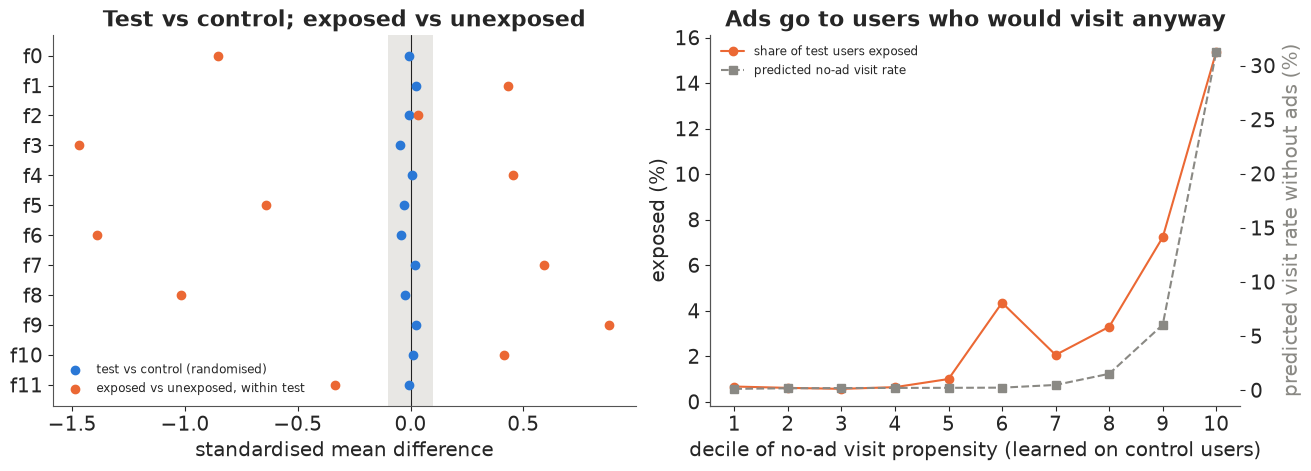
The left panel puts the two comparisons side by side on the same scale. Between the randomised arms every SMD is inside the grey band of $\pm 0.1$; between exposed and unexposed users, eleven of twelve features are outside it, five of them by more than 0.8 standard deviations. Exposed users are a different population.
The right panel shows what kind of difference. We fit a logistic model of visiting to the control arm, where nobody saw an ad, so its prediction is a user's no-ad visit propensity: a measure of how active and interested they already are. Applied to test users, it predicts a no-ad visit rate of 16.6% for those who were later exposed and 3.6% for those who were not. Ranking test users by it, the share exposed is at most 1% in the bottom half and 15.4% in the top decile. The campaign delivers its ads to the users who would have visited anyway. (The bump at the sixth decile is probably a point mass in the features: many users share the same values, so the decile cuts cannot split them.) That is the selection the propensity methods must undo, and the visit rate of the unexposed (3.5%) says nothing about what the exposed would have done.
D · A Bayesian propensity model for exposure
D1 · The respondent file
A vendor's survey file is not a random sample of the audience: it fills a quota of exposed respondents and a quota of unexposed ones. We mimic that by keeping every exposed test user in the sample and one unexposed test user in five. Such choice-based sampling changes the exposure rate in the file, but in a logistic model it changes only the intercept: if unexposed users are kept with probability $f$,
$$\operatorname{logit} P(D = 1 \mid x, \text{in file}) = \operatorname{logit} P(D = 1 \mid x) - \log f$$
(Prentice & Pyke 1979). We fit the model on the file and add $\log f$ back to get each user's propensity in the population. For the effect on the exposed the correction cancels anyway: unexposed respondents are weighted by the odds $e(x)/(1 - e(x))$ times $1/f$ for the sampling, and that product is exactly the odds the model predicts in the file.
F_UNEXP = 0.2
keep = tst & ((D == 1) | (rng.random(N) < F_UNEXP))
S = np.flatnonzero(keep)                         # the respondent file: all exposed + 1 in 5 unexposed, test arm
Zs, Ds = Zall[S], D[S]
Ys = {k: Y[k][S] for k in KPIS}
print(f"respondent file: {len(S):,} rows = {Ds.sum():,} exposed + {(1 - Ds).sum():,} unexposed "
      f"(sampling fraction {F_UNEXP} for the unexposed)")
for k in KPIS:
    print(f"  {k:10s}: {int(Ys[k][Ds == 1].sum()):5d} among exposed, {int(Ys[k][Ds == 0].sum()):5d} among unexposed")
respondent file: 58,161 rows = 9,122 exposed + 49,039 unexposed (sampling fraction 0.2 for the unexposed)
  visit     :  3705 among exposed,  1682 among unexposed
  conversion:   514 among exposed,    63 among unexposed
D2 · The model and its prior
The twelve features are awkward: f0 has 206,512 distinct values while f1 has 25, and most of them have a large point mass at one end and a long tail. We replace each by its rank-based normal score (ties share a rank), so a coefficient means the same thing for every feature, and we let each feature act through a linear and a quadratic term:
$$\operatorname{logit} P(D_i = 1) = a + \sum_j \beta_j\, r_{ij} + \sum_j \gamma_j\,(r_{ij}^2)^\ast, \qquad \beta_j \sim N(0, 0.5),\quad \gamma_j \sim N(0, \tau_q),\quad \tau_q \sim \text{HalfNormal}(0.5),$$
with every column standardised. The quadratic terms share a scale $\tau_q$ learned from the data, so the model can switch curvature off as a group (a small hierarchical touch), and $a \sim N(\operatorname{logit} \bar D_{\text{file}}, 1)$. The slopes' prior is deliberately modest: twelve standardised features with N(0, 1) slopes would put many users at propensities of 0 or 1 before seeing any data. We check what this prior implies for the population propensity by pushing prior draws through the design.
coords = {"feature": FEATS}
share = Ds.mean()


def propensity_model(Z, d):
    with pm.Model(coords=coords) as m:
        a = pm.Normal("a", special.logit(share), 1.0)
        b_lin = pm.Normal("b_lin", 0.0, 0.5, dims="feature")
        tau_q = pm.HalfNormal("tau_q", 0.5)
        b_quad = pm.Normal("b_quad", 0.0, tau_q, dims="feature")
        eta = a + Z[:, :12] @ b_lin + Z[:, 12:] @ b_quad
        pm.Bernoulli("exposed", logit_p=eta, observed=d)
    return m


prop_model = propensity_model(Zs, Ds)
with prop_model:
    prior = pm.sample_prior_predictive(draws=500, var_names=["a", "b_lin", "b_quad"], random_seed=RANDOM_SEED)
pa = prior.prior["a"].values.ravel()
pb = np.concatenate([prior.prior["b_lin"].values.reshape(-1, 12), prior.prior["b_quad"].values.reshape(-1, 12)], 1)
sub = rng.choice(len(Zs), 4000, replace=False)
eta_prior = pa[:, None] + pb @ Zs[sub].T + np.log(F_UNEXP)          # population propensity, logit scale
e_prior = special.expit(eta_prior)
print(f"prior predictive, population propensity: median {np.median(e_prior):.3f}; "
      f"share of users below 0.001 {np.mean(e_prior < 1e-3):.2f}, above 0.5 {np.mean(e_prior > 0.5):.2f}; "
      f"implied exposure rate 5-95%: {np.percentile(e_prior.mean(1), [5, 95]).round(3)}")
prior predictive, population propensity: median 0.039; share of users below 0.001 0.06, above 0.5 0.08; implied exposure rate 5-95%: [0.029 0.292]
The prior predictive puts the median user's propensity at 0.04, with 6% of users below 0.001 and 8% above 0.5, and an implied campaign-wide exposure rate anywhere between 3% and 29%. That is wide but not absurd: it allows extreme propensities without insisting on them. We sample with nutpie and a low-rank mass matrix (the 26 parameters are correlated through the features), and with 400 warm-up and 500 kept draws per chain instead of the default 1,000, because the 58,000-row likelihood is the slowest step in the notebook and the effective sample sizes below are ample.
t0 = time.time()
with prop_model:
    idata_prop = pm.sample(tune=400, draws=500, random_seed=RANDOM_SEED, progressbar=False,
                           nuts={"adaptation": "low_rank"})
print(f"sampled in {time.time() - t0:.0f} s; divergences {int(idata_prop.sample_stats['diverging'].sum())}; "
      f"warm-up {idata_prop.posterior.attrs.get('tuning_steps')}; "
      f"mean tree depth {float(idata_prop.sample_stats['depth'].mean()):.1f}")
summ = az.summary(idata_prop, ci_prob=0.9, round_to=3)
print(f"max r_hat {summ['r_hat'].max():.3f}, min bulk ESS {summ['ess_bulk'].min():.0f}")
print(summ.loc[["a", "tau_q"]])
bl = idata_prop.posterior["b_lin"].mean(("chain", "draw")).to_series()
bq = idata_prop.posterior["b_quad"].mean(("chain", "draw")).to_series()
print(pd.DataFrame({"linear": bl, "quadratic": bq}).round(2).T.to_string())
sampled in 67 s; divergences 0; warm-up 400; mean tree depth 3.0
max r_hat 1.008, min bulk ESS 3527
        mean     sd  eti90_lb  eti90_ub  ess_bulk  ess_tail  r_hat  mcse_mean  mcse_sd
a     -3.011  0.025    -3.053    -2.968  3526.704  1680.384  1.002      0.000    0.001
tau_q  0.205  0.051     0.137     0.301  3918.022  1638.453  1.001      0.001    0.001
feature      f0    f1    f2    f3    f4    f5    f6    f7    f8    f9   f10   f11
linear    -0.97 -0.05 -0.44 -0.72  0.02 -0.13 -1.17 -0.00 -0.77  0.12  0.02  0.02
quadratic  0.25  0.07  0.09 -0.27  0.09 -0.04 -0.21 -0.01 -0.37  0.05 -0.09  0.04
The fit is clean: no divergences, r_hat at most 1.008, bulk ESS at least 3,500, mean tree depth 3. The quadratic scale $\tau_q$ is about 0.2 (0.14-0.30), so curvature matters but is modest. The strongest signals are f6, f0, f8 and f3, four of the five features that differ most between exposed and unexposed users.
Now the checks. A propensity model is a prediction model, so we can ask whether its predictions are calibrated: sort the file into 20 bins by predicted probability, compare the observed share exposed with the prediction, and compare the gap with the posterior predictive spread.
post = az.extract(idata_prop, var_names=["a", "b_lin", "b_quad"], num_samples=400, random_seed=RANDOM_SEED)
A_draw = post["a"].values
B_draw = np.concatenate([post["b_lin"].values, post["b_quad"].values], 0)       # (24, draws)
eta_s = A_draw[None, :] + Zs @ B_draw                                           # sample-scale logit, (rows, draws)
eta_mean = eta_s.mean(1)
e_pop = special.expit(eta_mean + np.log(F_UNEXP))                               # population propensity
odds_s = np.exp(eta_s)                                                          # ATT weights for unexposed rows
w_mean = np.exp(eta_mean)

# calibration in the file: predicted vs observed exposure share in 20 bins
p_s = special.expit(eta_mean)
bins = pd.qcut(p_s, 20, labels=False, duplicates="drop")
calib = pd.DataFrame({"pred": pd.Series(p_s).groupby(bins).mean(), "obs": pd.Series(Ds).groupby(bins).mean(),
                      "n": pd.Series(Ds).groupby(bins).size()})
# posterior predictive spread of the observed share per bin
ppc_share = np.stack([pd.Series(rng.random(len(Ds)) < special.expit(eta_s[:, j])).groupby(bins).mean().values
                      for j in range(0, 400, 4)])
print(f"calibration: largest |obs - pred| over 20 bins {np.abs(calib.obs - calib.pred).max():.3f}; "
      f"bins outside the 90% predictive band: "
      f"{np.sum((calib.obs.values < np.percentile(ppc_share, 5, 0)) | (calib.obs.values > np.percentile(ppc_share, 95, 0)))}")
ue = Ds == 0
w_u = w_mean[ue]
ess_u = w_u.sum() ** 2 / (w_u ** 2).sum()
print(f"population propensity: exposed median {np.median(e_pop[Ds == 1]):.3f} "
      f"(1-99%: {np.percentile(e_pop[Ds == 1], 1):.4f}-{np.percentile(e_pop[Ds == 1], 99):.3f}); unexposed median "
      f"{np.median(e_pop[ue]):.4f} (99%: {np.percentile(e_pop[ue], 99):.3f})")
print(f"exposed with propensity above 0.9: {np.sum(e_pop[Ds == 1] > 0.9)} of {Ds.sum()}; "
      f"unexposed with weight share: top 1% of unexposed carry {np.sort(w_u)[-len(w_u) // 100:].sum() / w_u.sum():.2f} "
      f"of the weight; effective sample size {ess_u:,.0f} of {ue.sum():,}")
calibration: largest |obs - pred| over 20 bins 0.054; bins outside the 90% predictive band: 16
population propensity: exposed median 0.209 (1-99%: 0.0035-0.787); unexposed median 0.0066 (99%: 0.391)
exposed with propensity above 0.9: 1 of 9122; unexposed with weight share: top 1% of unexposed carry 0.28 of the weight; effective sample size 3,736 of 49,039
Xs = X[S]


def smd_w(Xm, d, w):
    m1 = Xm[d == 1].mean(0)
    m0 = np.average(Xm[d == 0], axis=0, weights=w)
    sd = np.sqrt((Xm[d == 1].var(0) + Xm[d == 0].var(0)) / 2)
    return (m1 - m0) / sd


bal = pd.DataFrame({"before": smd_w(Xs, Ds, np.ones(ue.sum())), "after weighting": smd_w(Xs, Ds, w_u)}, index=FEATS)
Rs = R[S]
bal["scores, after"] = smd_w(Rs, Ds, w_u)
print(bal.round(3).T.to_string())
print(f"max |SMD| before {bal.before.abs().max():.2f}, after (raw features) {bal['after weighting'].abs().max():.3f}, "
      f"after (normal scores) {bal['scores, after'].abs().max():.3f}")

fig, axes = plt.subplots(1, 3, figsize=(15, 4.4), gridspec_kw={"width_ratios": [1.2, 1, 1]})
ax = axes[0]
lb = np.linspace(-3.5, 0, 57)
ax.hist(np.log10(e_pop[ue]), bins=lb, density=True, color=BLUE, alpha=0.55, label="unexposed (test arm)")
ax.hist(np.log10(e_pop[Ds == 1]), bins=lb, density=True, color=ORANGE, alpha=0.55, label="exposed")
ax.set(xlabel="log10 propensity to be exposed (posterior mean)", ylabel="density",
       title="Overlap of the propensities")
ax.legend(fontsize=8.5)
ax = axes[1]
lo, hi = np.percentile(ppc_share, [5, 95], 0)
ax.fill_between(calib.pred, lo, hi, color=LIGHT, step="mid", label="90% posterior predictive")
ax.plot([0, 1], [0, 1], color=MUTED, lw=0.8)
ax.plot(calib.pred, calib.obs, "o", color=PURPLE, ms=4, label="observed share")
ax.set(xscale="log", yscale="log", xlim=(3e-3, 1), ylim=(3e-3, 1), xlabel="predicted P(exposed) in the file",
       ylabel="observed share exposed", title="Calibration (20 bins)")
ax.legend(fontsize=8.5)
ax = axes[2]
ax.scatter(bal.before, yy, color=ORANGE, s=30, label="before")
ax.scatter(bal["after weighting"], yy, color=AQUA, s=30, label="after ATT weighting")
ax.axvspan(-0.1, 0.1, color=LIGHT, alpha=0.6, lw=0)
ax.axvline(0, color=INK, lw=0.8)
ax.set(yticks=yy, yticklabels=FEATS, xlabel="standardised mean difference", title="Balance in the file")
ax.invert_yaxis()
ax.legend(fontsize=8.5);
                    f0     f1     f2     f3     f4     f5     f6     f7     f8     f9    f10    f11
before          -0.854  0.437  0.031 -1.475  0.456 -0.647 -1.389  0.592 -1.007  0.885  0.413 -0.340
after weighting -0.074  0.016 -0.008 -0.021  0.038 -0.013 -0.016 -0.021  0.049 -0.062 -0.017 -0.031
scores, after   -0.019  0.003 -0.010 -0.012  0.006  0.005 -0.021 -0.015  0.041 -0.061 -0.009 -0.005
max |SMD| before 1.47, after (raw features) 0.074, after (normal scores) 0.061
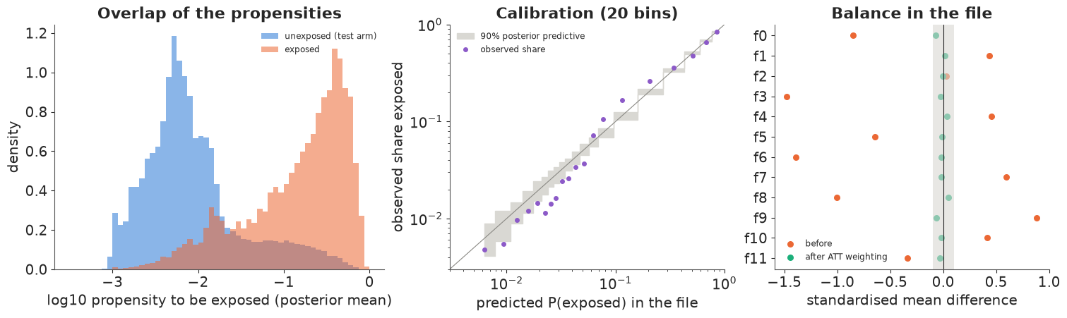
The calibration check fails. In 16 of 20 bins the observed share lies outside the 90% posterior predictive band; the model is too low in the middle of the range (around 0.1-0.3) and too high below 0.05, by up to 5 points. We keep the model anyway for now, because the question is whether the misfit matters for the answer, and part F tests exactly that with richer models.
Overlap is the other check. Positivity requires every exposed user to have comparable unexposed users, which on the propensity scale means unexposed users with similar propensities. The left panel shows the two distributions sitting thirty-fold apart: most unexposed mass lies between $10^{-3}$ and $10^{-1.5}$, most exposed mass between $10^{-1.5}$ and 1, and the exposed's long left tail reaches deep into the unexposed range. The median exposed user has a population propensity of 0.21, the median unexposed user 0.0066. The overlap is not broken - only 1 of 9,122 exposed users is above 0.9, and the unexposed reach 0.39 at their 99th percentile - but it is thin, and thin overlap is expensive: once reweighted to look like the exposed, the top 1% of unexposed users carry 28% of the weight, and the 49,039 unexposed respondents count as 3,736 effective ones.
Balance is the check the method is built for, and it passes. Weighting each unexposed respondent by their odds of exposure brings the largest SMD from 1.47 to 0.074 on the raw features (0.061 on the normal scores), every feature inside the 0.1 band. By the standard diagnostics of the propensity literature, the weighted unexposed now look like the exposed. Keep that in mind when we see the estimates.
E · Four estimates of the effect on the exposed
Every estimator of the effect on the exposed has the same shape: the exposed users' own outcome rate, which we observe, minus an estimate of the rate they would have had without ads, which we do not:
$$\tau = \bar Y_{D=1} - \widehat{E}\big[Y(0) \mid D = 1\big].$$
They differ in how they build that counterfactual from the unexposed:
- IPW weights unexposed respondents by their odds of exposure, $w_i = e(x_i)/(1 - e(x_i))$ (times $1/f$), and takes the weighted mean of their outcomes. We do not trim the weights: the unexposed propensities stay below about 0.4 at their 99th percentile, so the odds stay bounded.
- Stratification cuts the propensity scale into ten bands at the deciles of the exposed and compares exposed and unexposed within each band, weighting bands by their exposed counts (Rosenbaum & Rubin 1984).
- Outcome regression fits a model $m_0(x)$ of the outcome among the unexposed and averages its predictions over the exposed.
- AIPW (doubly robust; Robins, Rotnitzky & Zhao 1994) starts from outcome regression and corrects it with the weighted residuals of the unexposed: $\hat\tau = \overline{(Y - m_0)}_{D=1} - \sum_{D=0} w_i (Y_i - m_0(x_i)) / \sum_{D=0} w_i$. It is consistent if either the propensity or the outcome model is right.
The outcome models are Bayesian logistic regressions with the same 24 terms, fitted to the 49,039 unexposed respondents of each KPI.
Propagating uncertainty. A fully joint Bayesian model of exposure and outcome sounds natural, but it has a known flaw: the outcome model then feeds back into the propensity coefficients, which start to fit the outcome instead of the exposure, and the balancing property is lost (McCandless, Gustafson & Austin 2009; Zigler et al. 2013). The usual answer is a cut: fit the propensity model on exposure alone, then push each of its posterior draws through the estimator. That covers uncertainty about the propensities, but not the sampling variability of the outcomes themselves, which a plug-in estimator treats as fixed. For that we add the Bayesian bootstrap (Rubin 1981): for each draw, give every respondent an Exponential(1) weight - a draw from a Dirichlet posterior over the population of respondents. Pairing 400 propensity draws, 400 outcome-model draws and 400 bootstrap weightings gives 400 draws of each estimate. The rows marked "mean model" hold the propensity and outcome models at their posterior means, to show how much each source contributes.
def outcome_model(Z, y, name):
    with pm.Model(coords=coords, name=name) as m:
        a = pm.Normal("a", special.logit(max(y.mean(), 1e-3)), 1.5)
        b_lin = pm.Normal("b_lin", 0.0, 0.5, dims="feature")
        b_quad = pm.Normal("b_quad", 0.0, 0.5, dims="feature")
        pm.Bernoulli("y", logit_p=a + Z[:, :12] @ b_lin + Z[:, 12:] @ b_quad, observed=y)
    return m


m0_draws = {}
for k in KPIS:
    t0 = time.time()
    with outcome_model(Zs[ue], Ys[k][ue], k):
        idt = pm.sample(tune=400, draws=500, random_seed=RANDOM_SEED, progressbar=False,
                        nuts={"adaptation": "low_rank"})
    s_ = az.summary(idt, round_to=3)
    print(f"{k:10s} outcome model on {ue.sum():,} unexposed rows: {time.time() - t0:.0f} s, divergences "
          f"{int(idt.sample_stats['diverging'].sum())}, max r_hat {s_['r_hat'].max():.3f}, "
          f"min bulk ESS {s_['ess_bulk'].min():.0f}")
    po = az.extract(idt, var_names=[f"{k}::a", f"{k}::b_lin", f"{k}::b_quad"], num_samples=400,
                    random_seed=RANDOM_SEED + 1)
    Bo = np.concatenate([po[f"{k}::b_lin"].values, po[f"{k}::b_quad"].values], 0)
    m0_draws[k] = special.expit(po[f"{k}::a"].values[None, :] + Zs @ Bo)        # (rows, draws)
    del idt
visit outcome model on 49,039 unexposed rows: 53 s, divergences 0, max r_hat 1.013, min bulk ESS 4209
conversion outcome model on 49,039 unexposed rows: 46 s, divergences 0, max r_hat 1.010, min bulk ESS 3359
def estimators(y, d, w, m0, g, n_strata=10, e_rank=None):
    """ATT estimates for one draw: w = ATT weights (sample odds), m0 = predicted no-ad outcome,
    g = Bayesian-bootstrap weights over respondents."""
    t, u = d == 1, d == 0
    y1 = np.average(y[t], weights=g[t])
    out = {"naive": y1 - np.average(y[u], weights=g[u])}
    out["IPW"] = y1 - np.average(y[u], weights=g[u] * w[u])
    cuts = np.quantile(e_rank[t], np.linspace(0, 1, n_strata + 1)[1:-1])
    st = np.searchsorted(cuts, e_rank)
    est = tot = 0.0
    for s in range(n_strata):
        a_, b_ = t & (st == s), u & (st == s)
        if b_.any():
            est += g[a_].sum() * (np.average(y[a_], weights=g[a_]) - np.average(y[b_], weights=g[b_]))
            tot += g[a_].sum()
    out["stratification"] = est / tot
    out["outcome regression"] = np.average(y[t] - m0[t], weights=g[t])
    out["AIPW"] = out["outcome regression"] - np.average(y[u] - m0[u], weights=g[u] * w[u])
    out["AIPW baseline"] = y1 - out["AIPW"]           # the imputed no-ad rate of the exposed
    return out


rows = []
for j in range(400):
    g = rng.exponential(size=len(S))                       # Bayesian bootstrap (Rubin 1981)
    for k in KPIS:
        r_ = estimators(Ys[k], Ds, odds_s[:, j], m0_draws[k][:, j], g, e_rank=eta_s[:, j])
        rows += [{"kpi": k, "estimator": e_, "draw": j, "att": v} for e_, v in r_.items()]
    # the same quantities with the propensity draw held at its mean (bootstrap only)
    for k in KPIS:
        r_ = estimators(Ys[k], Ds, w_mean, m0_draws[k].mean(1), g, e_rank=eta_mean)
        rows += [{"kpi": k, "estimator": e_ + " [mean model]", "draw": j, "att": v} for e_, v in r_.items()]
est = pd.DataFrame(rows)
ORDER = ["naive", "IPW", "stratification", "outcome regression", "AIPW"]
tab = est.groupby(["kpi", "estimator"]).att.agg(mean="mean", lo=lambda v: v.quantile(0.05),
                                                 hi=lambda v: v.quantile(0.95), sd="std").reset_index()
for k in KPIS:
    t_ = tab[tab.kpi == k].set_index("estimator").loc[ORDER + [o + " [mean model]" for o in ORDER[1:]]]
    t_["vs truth"] = t_["mean"] - truth[k]
    print(f"--- {k}: experimental truth {truth[k]:.4f}")
    print(t_.drop(columns="kpi").round(4).to_string())
--- visit: experimental truth 0.2117
                                   mean      lo      hi      sd  vs truth
estimator
naive                            0.3718  0.3632  0.3801  0.0051    0.1601
IPW                              0.2516  0.2373  0.2666  0.0091    0.0399
stratification                   0.2552  0.2429  0.2692  0.0084    0.0435
outcome regression               0.2587  0.2475  0.2713  0.0073    0.0470
AIPW                             0.2605  0.2473  0.2740  0.0080    0.0488
IPW [mean model]                 0.2518  0.2380  0.2662  0.0084    0.0401
stratification [mean model]      0.2556  0.2422  0.2682  0.0081    0.0439
outcome regression [mean model]  0.2587  0.2515  0.2661  0.0043    0.0470
AIPW [mean model]                0.2605  0.2475  0.2735  0.0077    0.0488
--- conversion: experimental truth 0.0278
                                   mean      lo      hi      sd  vs truth
estimator
naive                            0.0551  0.0510  0.0595  0.0025    0.0273
IPW                              0.0469  0.0399  0.0529  0.0041    0.0191
stratification                   0.0478  0.0419  0.0534  0.0036    0.0200
outcome regression               0.0449  0.0391  0.0503  0.0034    0.0171
AIPW                             0.0455  0.0392  0.0518  0.0037    0.0177
IPW [mean model]                 0.0470  0.0402  0.0531  0.0039    0.0192
stratification [mean model]      0.0479  0.0419  0.0535  0.0035    0.0201
outcome regression [mean model]  0.0449  0.0410  0.0489  0.0024    0.0171
AIPW [mean model]                0.0454  0.0396  0.0512  0.0034    0.0176
iv_post = {k: idata_iv.posterior["att"].sel(kpi=k).values.ravel() for k in KPIS}
adj_post = {k: rng.normal(exp_s[k]["300k sample"], exp_s[k]["sd (sample)"], 4000) for k in KPIS}
fig, axes = plt.subplots(1, 2, figsize=(14, 4.8))
labels = ORDER + ["experiment, unadjusted (300k)", "experiment, adjusted (300k)"]
for ax, k in zip(axes, KPIS):
for i, e_ in enumerate(labels):
if e_.startswith("experiment"):
v = iv_post[k] if "unadjusted" in e_ else adj_post[k]
else:
v = est[(est.kpi == k) & (est.estimator == e_)].att.values
lo, hi = np.percentile(v, [5, 95])
col = (LIGHT if "unadjusted" in e_ else BLUE) if e_.startswith("experiment") else (
MUTED if e_ == "naive" else ORANGE)
ax.plot([lo * 100, hi * 100], [i, i], color=col, lw=3, solid_capstyle="round")
ax.plot(v.mean() * 100, i, "o", color=col if col != LIGHT else MUTED, ms=7)
ax.axvspan((truth[k] - 1.645 * truth_sd[k]) * 100, (truth[k] + 1.645 * truth_sd[k]) * 100, color=BLUE,
alpha=0.25)
ax.axvspan(truth_rng[k][0] * 100, truth_rng[k][1] * 100, color=BLUE, alpha=0.1) # range across bases
ax.axvline(truth[k] * 100, color=BLUE, lw=1.2)
ax.axvline(truth_unadj[k] * 100, color=MUTED, lw=1, ls=":")
ax.text(truth[k] * 100, -0.75, " experiment, all users, adjusted", color=BLUE, fontsize=8.5, va="center")
ax.text(truth_unadj[k] * 100, -0.35, " unadjusted", color=MUTED, fontsize=8, va="center")
ax.set(yticks=range(len(labels)), yticklabels=labels, ylim=(len(labels) - 0.4, -1.1),
xlabel=f"effect of the ad on the exposed: {k} (percentage points)", title=f"{k.capitalize()}")
fig.suptitle("Propensity estimates (orange) against the randomised answer (blue); 90% intervals");
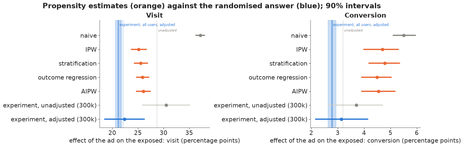
The four estimators agree with each other and disagree with the experiment.
For visits, every propensity estimate lands between 25.2 and 26.1 points, with 90% intervals about 3 points wide; the experiment's benchmark is 21.2, so they are 4-5 points (19-23%) too high, and none of their intervals reaches it. For conversions they give 4.5-4.8 points against a benchmark of 2.78, 61-72% too high, again with intervals that exclude the truth by a wide margin. The adjustment removed most of the naive bias for visits (37.2 points) and less of it for conversions (5.5 points). The experiment run on the same 300,000 users, adjusted as in part B, gives 22.4 and 3.15 with wide intervals that cover the benchmark; even unadjusted, its intervals are about three times wider than the propensity intervals for visits and half again as wide for conversions, and centred elsewhere. Against the unadjusted experimental answer (dotted), the propensity methods would look slightly low for visits and still far too high for conversions. The darker blue band in this and later figures is the benchmark's sampling uncertainty only; the lighter one spans the three adjusted bases of part B, a reminder that the answer key itself is known to about a point for visits.
Most of the posterior width comes from the respondents, not from the models. Holding the propensity model at its mean barely narrows IPW (sd 0.91 to 0.84 points for visits); holding the outcome model at its mean halves the width of outcome regression (0.73 to 0.43). Either way, the uncertainty that the Bayesian machinery propagates is the uncertainty given that the features contain every confounder. It says nothing about the error that matters here.
F · Why it fails
F1 · The disagreement lives in one number: what the exposed would have done anyway
p1_file = {k: Ys[k][Ds == 1].mean() for k in KPIS}
base = []
for k in KPIS:
    imp = est[(est.kpi == k) & (est.estimator == "AIPW baseline")].att.values
    base.append({"kpi": k, "exposed, with ads": p1_file[k], "unexposed (naive)": Ys[k][ue].mean(),
                 "propensity (AIPW)": imp.mean(),
                 "experiment, unadjusted": pc1_true[k] - truth_unadj[k],
                 "experiment, adjusted": pc0_true[k]})
base = pd.DataFrame(base).set_index("kpi")
print(base.round(4).to_string())
for k in KPIS:
    print(f"{k:10s}: selection bias of the naive baseline {base.loc[k, 'experiment, adjusted'] - base.loc[k, 'unexposed (naive)']:+.4f}; "
          f"left after propensity adjustment {base.loc[k, 'experiment, adjusted'] - base.loc[k, 'propensity (AIPW)']:+.4f}; "
          f"implied lift: experiment {pc1_true[k] / pc0_true[k]:.2f}x, propensity "
          f"{p1_file[k] / base.loc[k, 'propensity (AIPW)']:.1f}x")
            exposed, with ads  unexposed (naive)  propensity (AIPW)  experiment, unadjusted  experiment, adjusted
kpi
visit                  0.4062             0.0343             0.1456                  0.1275                0.2028
conversion             0.0563             0.0013             0.0109                  0.0218                0.0260
visit     : selection bias of the naive baseline +0.1685; left after propensity adjustment +0.0573; implied lift: experiment 2.04x, propensity 2.8x
conversion: selection bias of the naive baseline +0.0247; left after propensity adjustment +0.0151; implied lift: experiment 2.07x, propensity 5.2x
Every method agrees on what the exposed did with ads, 40.6% visiting and 5.6% converting in the file. They disagree only about the counterfactual. The naive comparison uses the unexposed rate, 3.4%; the propensity methods impute 14.6%; the adjusted experiment says 20.3% (12.75% unadjusted). For conversions: 0.13% naive, 1.09% propensity, 2.60% experiment (2.18% unadjusted).
Read as selection bias, the naive baseline is 16.9 points too low for visits; the propensity adjustment recovers 11.1 of them and leaves 5.7. For conversions the naive baseline is 2.5 points too low, and the adjustment recovers only 1.0 of them, leaving 1.5, which is why the conversion estimate is so much worse in relative terms. In the units a brand lift report uses, the propensity analysis says exposure made people 2.8 times as likely to visit and 5.2 times as likely to convert; the experiment says about 2.0 times for both.
The features capture who gets an ad well enough to balance them, and they capture activity well enough to remove most of the visit bias. What they do not capture is intent: whether a person was about to buy anyway. Criteo is a retargeting platform, so exposed users are likely people who recently showed interest, and that interest is visible to the ad platform's bidding but probably only partly in twelve anonymised features. A conversion is a sharper measure of intent than a visit, so the hidden part matters more for it.
F2 · More features move the answer, and nothing says when to stop
An analyst who suspects missing confounders adds features. We add them one at a time, most imbalanced first, refitting both models (posterior modes this time, with the same priors) and recomputing AIPW, and we also try random subsets of features, a model without the squares, and one with all 66 pairwise interactions.
def aipw_map(Z, d, ys, w_scale=1.0, prior_sd=0.5):
    """AIPW (Hajek form) with posterior-mode propensity and outcome models; returns {kpi: att}."""
    bp = fit_map(Z, d, prior_sd=prior_sd, a0=special.logit(d.mean()))
    Z1 = np.column_stack([np.ones(len(Z)), Z])
    eta = Z1 @ bp
    w = np.exp(eta - eta[d == 0].max()) * w_scale                 # weights enter only normalised averages
    t, u = d == 1, d == 0
    out = {}
    for k, y in ys.items():
        bo = fit_map(Z[u], y[u], prior_sd=prior_sd, a0=special.logit(max(y[u].mean(), 1e-4)))
        m0 = special.expit(Z1 @ bo)
        out[k] = np.mean(y[t] - m0[t]) - np.average(y[u] - m0[u], weights=w[u])
    return out


def design(cols, quad=True):
    return Zs[:, list(cols) + ([12 + c for c in cols] if quad else [])] if cols else np.zeros((len(S), 0))


order = list(np.argsort(-np.abs(smd["exposed vs unexposed"].values)))
t0 = time.time()
path = [{"k": 0, **{k: base.loc[k, "exposed, with ads"] - base.loc[k, "unexposed (naive)"] for k in KPIS}}]
for i in range(1, 13):
    path.append({"k": i, **aipw_map(design(order[:i]), Ds, Ys)})
path = pd.DataFrame(path)
path["added"] = ["-"] + [FEATS[c] for c in order]
cloud = []
for kk in (2, 4, 6, 8, 10):
    for r_ in range(8):
        cols = sorted(rng.choice(12, kk, replace=False))
        cloud.append({"k": kk, **aipw_map(design(cols), Ds, Ys)})
cloud = pd.DataFrame(cloud)
lin_only = aipw_map(design(range(12), quad=False), Ds, Ys)
pairs = np.column_stack([Zs[:, i] * Zs[:, j] for i, j in itertools.combinations(range(12), 2)])
pairs = (pairs - pairs.mean(0)) / pairs.std(0)
inter = aipw_map(np.column_stack([Zs, pairs]), Ds, Ys)


def calib_misses(Z):
    """Bins (of 20) where the observed exposed share is outside +-1.645 binomial sd of the predicted one."""
    eta_ = np.column_stack([np.ones(len(Z)), Z]) @ fit_map(Z, Ds, a0=special.logit(Ds.mean()))
    p_ = special.expit(eta_)
    b_ = pd.qcut(p_, 20, labels=False, duplicates="drop")
    c_ = pd.DataFrame({"p": p_, "d": Ds}).groupby(b_).agg(p=("p", "mean"), d=("d", "mean"), n=("d", "size"))
    return int(np.sum(np.abs(c_.d - c_.p) > 1.645 * np.sqrt(c_.p * (1 - c_.p) / c_.n)))


print(f"calibration misses (of 20 bins): squares model {calib_misses(Zs)}, "
      f"with interactions {calib_misses(np.column_stack([Zs, pairs]))}")
print(f"{len(path) + len(cloud) + 2} specifications in {time.time() - t0:.0f} s")
print(path.round(4).to_string(index=False))
print("random feature subsets (AIPW), min-max by size:")
print(cloud.groupby("k").agg(["min", "max"]).round(4).to_string())
print(f"all 12, linear terms only: {pd.Series(lin_only).round(4).to_dict()}")
print(f"all 12 + squares + 66 pairwise interactions: {pd.Series(inter).round(4).to_dict()}")
calibration misses (of 20 bins): squares model 16, with interactions 10
55 specifications in 8 s
 k  visit  conversion added
 0 0.3719      0.0551     -
 1 0.3301      0.0529    f3
 2 0.3448      0.0601    f6
 3 0.2731      0.0503    f8
 4 0.2635      0.0504    f9
 5 0.2641      0.0497    f0
 6 0.2649      0.0502    f5
 7 0.2648      0.0503    f7
 8 0.2639      0.0458    f4
 9 0.2639      0.0460    f1
10 0.2642      0.0458   f10
11 0.2636      0.0461   f11
12 0.2600      0.0455    f2
random feature subsets (AIPW), min-max by size:
     visit         conversion
       min     max        min     max
k
2   0.2530  0.3669     0.0437  0.0512
4   0.2721  0.3173     0.0465  0.0545
6   0.2502  0.2714     0.0439  0.0493
8   0.2523  0.2853     0.0439  0.0471
10  0.2593  0.2663     0.0439  0.0468
all 12, linear terms only: {'visit': 0.2829, 'conversion': 0.045}
all 12 + squares + 66 pairwise interactions: {'visit': 0.2582, 'conversion': 0.0443}fig, axes = plt.subplots(1, 2, figsize=(14, 4.5))
for ax, k in zip(axes, KPIS):
ax.axhspan((truth[k] - 1.645 * truth_sd[k]) * 100, (truth[k] + 1.645 * truth_sd[k]) * 100, color=BLUE,
alpha=0.25)
ax.axhspan(truth_rng[k][0] * 100, truth_rng[k][1] * 100, color=BLUE, alpha=0.1) # range across bases
ax.axhline(truth[k] * 100, color=BLUE, lw=1.2, label="experiment, adjusted (all users)")
ax.axhline(truth_unadj[k] * 100, color=MUTED, lw=1, ls=":", label="experiment, unadjusted")
ax.scatter(cloud.k + rng.uniform(-0.15, 0.15, len(cloud)), cloud[k] * 100, color=LIGHT, edgecolor=MUTED, s=22,
label="random feature subsets")
ax.plot(path.k, path[k] * 100, "o-", color=ORANGE, label="adding features, most imbalanced first")
ax.plot([12.35], [lin_only[k] * 100], "s", color=PURPLE, label="all 12, no squares")
ax.plot([12.6], [inter[k] * 100], "D", color=RED, label="all 12 + 66 interactions")
for i, r_ in path.iterrows():
if i:
ax.annotate(r_.added, (r_.k, r_[k] * 100), textcoords="offset points", xytext=(0, 7), fontsize=7,
ha="center", color=MUTED)
ax.set(xlabel="features in the propensity and outcome models", ylabel="AIPW effect on the exposed (pp)",
title=k.capitalize(), xticks=range(13))
axes[0].legend(fontsize=8, loc="upper right");
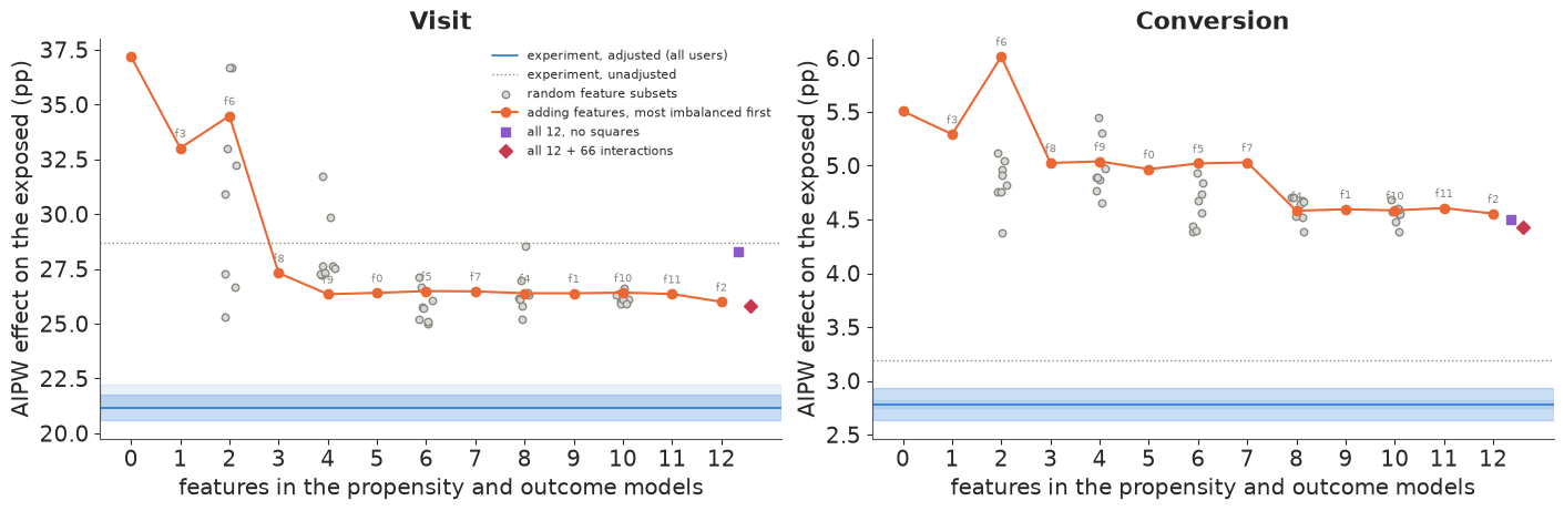
The ladder tells the usual story at first. Adding f3, the most imbalanced feature, moves the visit estimate from 37.2 to 33.0 points; adding f8 as the third brings it to 27.3; from four features on it sits between 26.0 and 26.5 and stays there. The random subsets spread widely with two features (25.3-36.7 points) and close in as features are added. An analyst watching this would see the estimate converge and stop, reasonably. It converges to the wrong place: the benchmark is 21.2, and none of the 55 specifications comes within 3.8 points of it - the lowest is 25.0. On the way down the ladder crosses the unadjusted experimental answer at three features, which shows the other danger: had that been the truth, a three-feature model would have looked nearly right by luck.
Flexibility does not help either. Dropping the squares gives 28.3; adding all 66 pairwise interactions gives 25.8, and the interactions reduce the calibration failure of part D (bins outside the band fall from 16 to 10) while moving the estimate by 0.2 points. A better model of who gets an ad is not a better model of what they would have done without one.
Conversions show the same pattern more starkly: every specification lies between 4.4 and 6.0 points against a benchmark of 2.78. The features that finish the visit adjustment have almost nothing left to say about purchase intent. Nothing in the observational data marks the right number of features, because the quantity that would tell us - the exposed users' no-ad outcome - is exactly what is missing.
G · How strong would the hidden confounder have to be?
A sensitivity analysis asks how much unmeasured confounding it would take to change the conclusion. The simplest version is the E-value (VanderWeele & Ding 2017): for an observed risk ratio $RR > 1$,
$$E = RR + \sqrt{RR\,(RR - 1)}$$
is the strength (as a risk ratio with both exposure and outcome) that an unmeasured confounder would need, above and beyond the measured features, to explain the association away. We can also ask what it takes to move the propensity estimate to the experiment's: divide the two risk ratios and compute the E-value of the ratio.
The second version builds the bias into the model. Let the true no-ad rate of the exposed differ from the propensity-imputed one by a log odds ratio $\delta$:
$$\operatorname{logit} q_{\text{true}} = \operatorname{logit} q_{\text{imputed}} + \delta, \qquad \tau = p_1 - q_{\text{true}}.$$
The observational data say nothing about $\delta$ - the exposed's counterfactual is never observed - so its posterior is its prior. We fit the model in PyMC with the imputed rate entering as a noisy measurement (its posterior mean and sd from part E), the exposed rate from its binomial counts, and four priors for $\delta$ with standard deviations 0.1, 0.25, 0.5 and 1.
def e_value(rr):
    rr = np.where(rr < 1, 1 / rr, rr)
    return rr + np.sqrt(rr * (rr - 1))


for k in KPIS:
    rr_obs = p1_file[k] / base.loc[k, "propensity (AIPW)"]
    rr_true = pc1_true[k] / pc0_true[k]
    print(f"{k:10s}: risk ratio, propensity {rr_obs:.2f}; E-value to explain it away {e_value(rr_obs):.1f}; "
          f"bias factor separating it from the experiment {rr_obs / rr_true:.2f} -> E-value {e_value(rr_obs / rr_true):.2f}")
visit     : risk ratio, propensity 2.79; E-value to explain it away 5.0; bias factor separating it from the experiment 1.37 -> E-value 2.07
conversion: risk ratio, propensity 5.18; E-value to explain it away 9.8; bias factor separating it from the experiment 2.50 -> E-value 4.44
q_imp = {k: est[(est.kpi == k) & (est.estimator == "AIPW baseline")].att.values for k in KPIS}
lq_mu = np.array([special.logit(q_imp[k]).mean() for k in KPIS])
lq_sd = np.array([special.logit(q_imp[k]).std() for k in KPIS])
print(f"imputed no-ad rate of the exposed, logit scale: mean {lq_mu.round(3)}, sd {lq_sd.round(3)}")
n1 = int(Ds.sum())
y1 = np.array([int(Ys[k][Ds == 1].sum()) for k in KPIS])
SCALES = [0.1, 0.25, 0.5, 1.0]
with pm.Model(coords={"kpi": KPIS, "scale": [str(s) for s in SCALES]}) as sens:
    p1 = pm.Beta("p1", 1.0, 1.0, dims="kpi")
    pm.Binomial("y1", n=n1, p=p1, observed=y1, dims="kpi")
    lq = pm.Normal("logit_q", -3.0, 2.0, dims=("scale", "kpi"))          # true no-ad rate of the exposed
    delta = pm.Normal("delta", 0.0, np.array(SCALES)[:, None], dims=("scale", "kpi"))
    pm.Normal("imputed", mu=lq - delta, sigma=lq_sd, observed=np.tile(lq_mu, (len(SCALES), 1)), dims=("scale", "kpi"))
    pm.Deterministic("att", p1 - pm.math.invlogit(lq), dims=("scale", "kpi"))
    idata_sens = pm.sample(random_seed=RANDOM_SEED, progressbar=False)
print(f"divergences {int(idata_sens.sample_stats['diverging'].sum())}")
att_s = idata_sens.posterior["att"]
need = {k: special.logit(pc0_true[k]) - lq_mu[i] for i, k in enumerate(KPIS)}
print("delta that would reconcile the propensity estimate with the experiment:",
      {k: round(float(v), 2) for k, v in need.items()})
sens_tab = []
for s in SCALES:
    for k in KPIS:
        v = att_s.sel(scale=str(s), kpi=k).values.ravel()
        lo, hi = np.percentile(v, [5, 95])
        sens_tab.append({"prior sd of delta": s, "kpi": k, "mean": v.mean(), "5%": lo, "95%": hi,
                         "covers truth": lo <= truth[k] <= hi})
print(pd.DataFrame(sens_tab).round(4).to_string(index=False))
dp = idata_sens.posterior["delta"].sel(scale="1.0")
print(f"posterior sd of delta at prior sd 1.0: {dp.std(('chain', 'draw')).values.round(3)} (the data never see it)")

fig, axes = plt.subplots(1, 2, figsize=(13, 4.2))
dg = np.linspace(-1.0, 2.0, 121)
for i, (ax, k) in enumerate(zip(axes, KPIS)):
    curve = p1_file[k] - special.expit(lq_mu[i] + dg)
    ax.plot(dg, curve * 100, color=ORANGE, lw=2, label="propensity estimate if the hidden bias were delta")
    ax.axhspan((truth[k] - 1.645 * truth_sd[k]) * 100, (truth[k] + 1.645 * truth_sd[k]) * 100, color=BLUE,
               alpha=0.25)
    ax.axhspan(truth_rng[k][0] * 100, truth_rng[k][1] * 100, color=BLUE, alpha=0.1)   # range across bases
    ax.axhline(truth[k] * 100, color=BLUE, lw=1.2, label="experiment, adjusted")
    ax.axvline(0, color=MUTED, lw=0.8, ls=":")
    ax.axvline(need[k], color=BLUE, lw=0.8, ls="--")
    ax.annotate(f"delta = {need[k]:.2f}\n(odds x {np.exp(need[k]):.1f})", (need[k], truth[k] * 100),
                textcoords="offset points", xytext=(8, 12), fontsize=8.5, color=BLUE)
    ax.set(xlabel="delta: log odds ratio, true vs imputed no-ad rate of the exposed",
           ylabel="effect on the exposed (pp)", title=k.capitalize())
axes[0].legend(fontsize=8.5, loc="lower left");
imputed no-ad rate of the exposed, logit scale: mean [-1.771 -4.545], sd [0.056 0.275]
divergences 0
delta that would reconcile the propensity estimate with the experiment: {'visit': 0.4, 'conversion': 0.92}
 prior sd of delta        kpi   mean      5%    95%  covers truth
              0.10      visit 0.2607  0.2349 0.2844         False
              0.10 conversion 0.0452  0.0383 0.0512         False
              0.25      visit 0.2613  0.2053 0.3069          True
              0.25 conversion 0.0447  0.0358 0.0520         False
              0.50      visit 0.2596  0.1448 0.3417          True
              0.50 conversion 0.0429  0.0272 0.0528          True
              1.00      visit 0.2662  0.0579 0.3750          True
              1.00 conversion 0.0342 -0.0128 0.0542          True
posterior sd of delta at prior sd 1.0: [0.849 0.923] (the data never see it)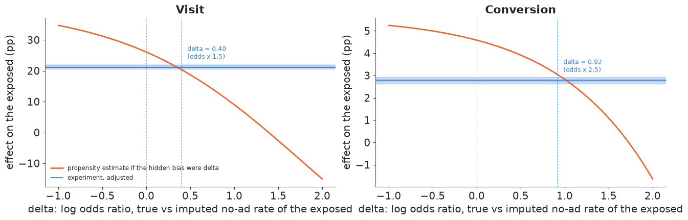
The E-values are large in one sense and small in another. To explain the whole conversion association away, a hidden confounder would need risk ratios of 9.8 with both exposure and conversion; for visits, 5.0. Nobody should conclude the ads did nothing. But to move the propensity estimate to the experiment's answer takes much less: an E-value of 2.1 for visits and 4.4 for conversions. In the bias model the gap is $\delta = 0.40$ for visits and 0.92 for conversions: the exposed's true no-ad odds of converting are 2.5 times what the propensity model imputes. "Intent to buy" in a retargeting campaign is easily that strong. The figure draws the whole curve: the estimate falls steadily as $\delta$ grows and crosses the benchmark at those two values.
The posterior of $\delta$ is essentially its prior (sd 0.85 and 0.92 against 1.0; the prior on the true rate trims the tails), which is the formal way of saying the data cannot learn it. Its prior therefore sets the width of the answer. With a prior sd of 0.1 - a near-certain belief that the features caught everything - neither interval covers the benchmark. Covering it takes a prior sd of 0.25 for visits (interval 20.5-30.7 points) and 0.5 for conversions (2.7-5.3). The honest observational report is then an interval two to four times as wide as the propensity analysis printed (about 10 points against 2.7 for visits, 2.6 against 1.3 for conversions), and how wide is a matter of opinion about $\delta$ that only an experiment can settle. Gordon et al. (2019) found that the size of the bias varied widely from campaign to campaign; that is the same finding from the other side.
H · Survey-sized samples: noisy and right, or tight and wrong
So far we have used hundreds of thousands of users. A real brand lift survey has a few thousand respondents. To see what happens at that size we replay the study: draw a simple random sample of $n$ users from the 300,000 (respondents of both arms), run both analyses on it, and repeat 100 times for each of $n$ = 2,000, 6,000, 20,000 and 60,000. The experimental analysis is the adjusted Wald estimate of part B (with linear terms only, fitted on the survey's control respondents), with a large-sample sd; the observational one is AIPW on the survey's test respondents with posterior-mode models, with the usual influence-function sd that treats the fitted models as known. Surveys of 60,000 are a fifth of the pool, so replays overlap and their spread is slightly understated.
def replay(n, rng_):
    idx = rng_.choice(N, n, replace=False)
    c_, t_ = idx[T[idx] == 0], idx[T[idx] == 1]
    out = {"n": n}
    Zc1, Zt1 = Zb[c_, :13], Zb[t_, :13]
    e_t = D[t_].mean()
    for k in KPIS:
        att, sd, _, _ = wald(len(c_), Y[k][c_].sum(), len(t_), D[t_].sum(), Y[k][t_].sum())
        out[f"wald_{k}"], out[f"wald_sd_{k}"] = att, sd
        # adjusted as in B3, linear terms only (squares made a few small surveys explode), fitted on the
        # survey's control respondents
        bc = np.linalg.lstsq(Zc1, Y[k][c_], rcond=None)[0]
        r_t = Y[k][t_] - Zt1 @ bc
        r_c = Y[k][c_] - Zc1 @ bc
        att = r_t.mean() / e_t
        out[f"rct_{k}"] = att
        out[f"rct_sd_{k}"] = np.sqrt(np.var(r_t - D[t_] * att) / len(t_) + np.var(r_c) / len(c_)) / e_t
    Z, d = Zall[t_], D[t_]
    bp = fit_map(Z, d, a0=special.logit(max(d.mean(), 1e-3)))
    Z1 = np.column_stack([np.ones(len(Z)), Z])
    eta = Z1 @ bp
    w = np.exp(eta - eta[d == 0].max())
    tt, uu = d == 1, d == 0
    for k in KPIS:
        y = Y[k][t_]
        bo = fit_map(Z[uu], y[uu], a0=special.logit(max(y[uu].mean(), 1e-4)))
        m0 = special.expit(Z1 @ bo)
        att = np.mean(y[tt] - m0[tt]) - np.average(y[uu] - m0[uu], weights=w[uu])
        # influence-function sd (nuisance models treated as known)
        mu_w = np.average(y[uu] - m0[uu], weights=w[uu])
        phi = (tt * (y - m0 - (att + mu_w)) - uu * w * (y - m0 - mu_w) * tt.sum() / w[uu].sum()) / tt.mean()
        out[f"ps_{k}"], out[f"ps_sd_{k}"] = att, phi.std() / np.sqrt(len(y))
    return out


SIZES, REPS = [2_000, 6_000, 20_000, 60_000], 100
t0 = time.time()
rr = np.random.default_rng(RANDOM_SEED + 7)
reps = pd.DataFrame([replay(n, rr) for n in SIZES for _ in range(REPS)])
print(f"{len(reps)} replays in {time.time() - t0:.0f} s")
z90 = stats.norm.ppf(0.95)
summ_rep = []
for n in SIZES:
    r_ = reps[reps.n == n]
    for meth in ("wald", "rct", "ps"):
        for k in KPIS:
            v, s = r_[f"{meth}_{k}"], r_[f"{meth}_sd_{k}"]
            summ_rep.append({"n": n, "design": {"wald": "experiment, unadjusted", "rct": "experiment, adjusted",
                                                "ps": "propensity (AIPW)"}[meth],
                             "kpi": k, "mean": v.mean(), "sd across surveys": v.std(), "median stated sd": s.median(),
                             "90% coverage": np.mean(np.abs(v - truth[k]) <= z90 * s),
                             "coverage with the true spread": np.mean(np.abs(v - truth[k]) <= z90 * v.std())})
summ_rep = pd.DataFrame(summ_rep)
print(summ_rep.round(4).to_string(index=False))
400 replays in 31 s
    n                 design        kpi   mean  sd across surveys  median stated sd  90% coverage  coverage with the true spread
 2000 experiment, unadjusted      visit 0.2731             0.3706            0.3529          0.87                           0.91
 2000 experiment, unadjusted conversion 0.0227             0.0921            0.0486          0.77                           0.92
 2000   experiment, adjusted      visit 0.2010             0.3410            0.2961          0.82                           0.91
 2000   experiment, adjusted conversion 0.0254             0.0972            0.0471          0.72                           0.93
 2000      propensity (AIPW)      visit 0.2643             0.0712            0.0656          0.74                           0.79
 2000      propensity (AIPW) conversion 0.0467             0.0336            0.0305          0.89                           0.85
 6000 experiment, unadjusted      visit 0.3044             0.1798            0.1892          0.85                           0.84
 6000 experiment, unadjusted conversion 0.0360             0.0421            0.0449          0.84                           0.92
 6000   experiment, adjusted      visit 0.2439             0.1705            0.1626          0.88                           0.86
 6000   experiment, adjusted conversion 0.0315             0.0456            0.0403          0.80                           0.96
 6000      propensity (AIPW)      visit 0.2653             0.0371            0.0373          0.56                           0.55
 6000      propensity (AIPW) conversion 0.0465             0.0198            0.0176          0.64                           0.69
20000 experiment, unadjusted      visit 0.2934             0.1137            0.1079          0.83                           0.84
20000 experiment, unadjusted conversion 0.0336             0.0231            0.0246          0.88                           0.90
20000   experiment, adjusted      visit 0.2156             0.1041            0.0932          0.88                           0.92
20000   experiment, adjusted conversion 0.0288             0.0249            0.0234          0.88                           0.93
20000      propensity (AIPW)      visit 0.2655             0.0362            0.0203          0.27                           0.67
20000      propensity (AIPW) conversion 0.0481             0.0150            0.0095          0.34                           0.74
60000 experiment, unadjusted      visit 0.3030             0.0534            0.0619          0.62                           0.50
60000 experiment, unadjusted conversion 0.0360             0.0117            0.0144          0.85                           0.78
60000   experiment, adjusted      visit 0.2244             0.0487            0.0538          0.93                           0.93
60000   experiment, adjusted conversion 0.0312             0.0125            0.0138          0.92                           0.86
60000      propensity (AIPW)      visit 0.2653             0.0219            0.0117          0.01                           0.05
60000 propensity (AIPW) conversion 0.0497 0.0084 0.0056 0.02 0.10fig, axes = plt.subplots(1, 2, figsize=(14, 4.6))
for ax, k in zip(axes, KPIS):
ax.axhline(truth[k] * 100, color=BLUE, lw=1.2, label="experiment, all users (adjusted)")
for meth, col, dx, lab in [("rct", BLUE, -0.04, "experiment, adjusted"), ("ps", ORANGE, 0.04, "propensity (AIPW)")]:
for n in SIZES:
v = reps[reps.n == n][f"{meth}_{k}"].values * 100
x = np.log10(n) + dx
ax.scatter(np.full(len(v), x) + rng.uniform(-0.015, 0.015, len(v)), v, s=5, color=col, alpha=0.3, lw=0)
ax.plot([x, x], np.percentile(v, [5, 95]), color=col, lw=2.5)
ax.plot(x, v.mean(), "o", color=col, ms=7, mec="white", label=lab if n == SIZES[0] else None)
cov = summ_rep[(summ_rep.n == n) & (summ_rep.kpi == k) & (summ_rep.design == (
"experiment, adjusted" if meth == "rct" else "propensity (AIPW)"))]["90% coverage"].iloc[0]
ax.annotate(f"{cov:.0%}", (x, np.percentile(v, 95)), textcoords="offset points", xytext=(0, 4),
fontsize=7.5, ha="center", color=col)
lim = {"visit": (-40, 100), "conversion": (-15, 20)}[k]
ax.set(xticks=np.log10(SIZES), xticklabels=[f"{n:,}" for n in SIZES], ylim=lim,
xlabel="respondents in the survey (random sample of the audience)",
ylabel="estimated effect on the exposed (pp)", title=f"{k.capitalize()} (labels: 90% interval coverage)")
axes[0].legend(fontsize=8, loc="upper right");
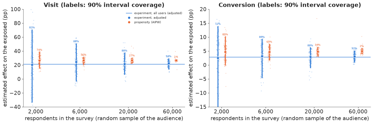
The figure is the notebook's argument in one picture. The experiment (blue) is noisy and centred: its replays average 20.1, 24.4, 21.6 and 22.4 points for visits as the survey grows from 2,000 to 60,000 respondents, and 2.5-3.2 points for conversions, around benchmarks of 21.2 and 2.78. At 2,000 respondents it is nearly useless - the middle 90% of replays runs from about -34 to +71 points for visits - but its intervals know it: they cover the benchmark in 82-93% of visit replays. For conversions at small sizes coverage falls to 72-80% because the large-sample sd is too optimistic with a handful of converters in control (4.7 points stated against 9.7 observed at 2,000); by 20,000 it is back near 90%.
The propensity analysis (orange) is tight and wrong, and it does not get less wrong. Its replays average 26.4-26.6 points for visits and 4.7-5.0 for conversions at every size. More respondents only shrink the spread, from 7.1 to 2.2 points for visits, around the same wrong centre, so coverage collapses: 74%, 56%, 27% and 1% for visits and 89%, 64%, 34% and 2% for conversions. Its stated sds are also too small at the larger sizes (they ignore the fitting of the two models), but even intervals built from the true spread would cover only 5% and 10% of replays at 60,000. This is bias, not noise.
At a few thousand respondents the propensity estimate actually looks better: its error is smaller than the experiment's noise. A brand manager choosing by interval width alone would pick it every time. The difference is that more data fixes the experiment and cannot fix the propensity analysis. (The unadjusted experiment, in the table, shows this file's imbalance in miniature: centred near 27-30 points for visits, with coverage down to 62% at 60,000.)
The experiment's noise at survey size is a design problem with a design solution. An intent-to-treat survey compares everyone in test with everyone in control, and 96% of both are people the campaign never reached, adding noise and no signal. Below, one survey of 6,000 respondents run through the Bayesian IV model of part B, and then the standard deviation the same survey would have if it compared only the exposed with the control users who would have been exposed.
surv = rng.choice(N, 6_000, replace=False)
with iv_model(counts(surv[T[surv] == 0], surv[T[surv] == 1])):
    idata_iv_s = pm.sample(random_seed=RANDOM_SEED, progressbar=False)
print(f"one survey of 6,000: divergences {int(idata_iv_s.sample_stats['diverging'].sum())}")
print(az.summary(idata_iv_s, var_names=["att", "p_c0"], ci_prob=0.9, round_to=4))

ghost = []
for n in SIZES:
    for k in KPIS:
        p1_, p0_ = pc1_true[k], pc0_true[k]
        sd_g = np.sqrt(p1_ * (1 - p1_) / (n / 2) + p0_ * (1 - p0_) / (n / 2))
        sd_itt = summ_rep[(summ_rep.n == n) & (summ_rep.kpi == k) & (summ_rep.design == "experiment, adjusted")][
            "sd across surveys"].iloc[0]
        ghost.append({"n": n, "kpi": k, "ITT design sd": sd_itt, "ghost-ad design sd": sd_g, "ratio": sd_itt / sd_g})
print(pd.DataFrame(ghost).round(4).to_string(index=False))
one survey of 6,000: divergences 0
                    mean      sd  eti90_lb  eti90_ub   ess_bulk   ess_tail   r_hat  mcse_mean  mcse_sd
att[visit]        0.3020  0.1059    0.0967    0.4344  4805.5278  2808.3365  1.0002     0.0014   0.0019
att[conversion]  -0.0168  0.0483   -0.1094    0.0392  4607.0748  2846.6413  1.0009     0.0007   0.0011
p_c0[visit]       0.1132  0.0991    0.0064    0.3137  3811.8114  2225.2731  1.0005     0.0014   0.0019
p_c0[conversion]  0.0562  0.0467    0.0052    0.1442  2841.9345  1548.4712  1.0006     0.0007   0.0012
    n        kpi  ITT design sd  ghost-ad design sd   ratio
 2000      visit         0.3410              0.0201 16.9595
 2000 conversion         0.0972              0.0087 11.1411
 6000      visit         0.1705              0.0116 14.6850
 6000 conversion         0.0456              0.0050  9.0463
20000      visit         0.1041              0.0064 16.3666
20000 conversion         0.0249              0.0028  9.0143
60000      visit         0.0487              0.0037 13.2687
60000 conversion         0.0125              0.0016  7.8141
One survey of 6,000 respondents gives a visit effect of 30 points with a 90% interval of 10-43, and a conversion effect of -1.7 points (-10.9 to 3.9): a survey that cannot tell whether the ads helped or hurt sales. That is the intent-to-treat design at survey size.
A ghost-ad design (Johnson, Lewis & Nubbemeyer 2017) fixes the comparison rather than the sample size. The ad platform runs its auction for control users too and logs when it would have shown the ad, so the control users who would have been exposed are known, and the survey can be split between exposed test users and their would-be-exposed controls. With the benchmark rates (41.5% vs 20.3% for visits, 5.4% vs 2.6% for conversions) and the respondents split evenly, the standard deviation of the effect on the exposed is 8-17 times smaller than the intent-to-treat design's: at 6,000 respondents, 1.2 points instead of 17 for visits, 0.5 instead of 4.6 for conversions. The table is a calculation, not a replay - Criteo's file does not record ghost impressions - but it shows the scale of what a better control group buys.
I · What the brand manager should report
The brand manager asked whether the ads worked. Here is what each analysis would have told them.
The naive survey comparison says exposure raised visits by 38 points and conversions by 5.3 points, lifts of 12 and 45 times. It is not an estimate of anything causal.
The propensity-adjusted study, done by the book - a Bayesian model with clean sampling, balance within 0.1 on every feature, four estimators that agree, uncertainty propagated - reports 26 points and 4.5 points, lifts of 2.8 and 5.2 times, with tight intervals. It overstates both, and the conversion lift by more than double. The one diagnostic that failed, calibration, did not point to the bias: improving it barely moved the estimate.
The experiment reports 21 points and 2.8 points, lifts of about 2.0 times, once the arms' small imbalance is adjusted for. Its own lesson is smaller but real: even a randomised file needs a balance check.
So the report should be built on the holdout: the campaign raised the exposed users' visit rate from about 20% to 41% and their conversion rate from about 2.6% to 5.4% in this file, roughly a doubling. The propensity numbers should not appear in it, not even as a cross-check, because agreement between observational estimators says nothing about their shared bias.
For the next study the design matters more than the analysis. Keep a randomised holdout, even a small one: it is what turned this notebook from guesswork into a measurement. Survey the right control respondents: an intent-to-treat survey wastes 96% of its sample on people the campaign never reached, so it needs hundreds of thousands of respondents to say anything. A ghost-ad or PSA design (Johnson, Lewis & Nubbemeyer 2017) records which control users would have been shown the ad, so the survey can compare the exposed with their randomised counterparts directly, and part H shows that buys an 8-17 fold reduction in the experiment's standard deviation at the same number of respondents. If no holdout is possible at all, report the observational estimate with a sensitivity interval for $\delta$, and calibrate that interval on past campaigns that did have a holdout.
print(f"total run time {time.time() - T_START:.0f} s")
total run time 239 s
Summary
- The naive exposed-versus-unexposed comparison is selection, not lift. Exposed users visited at 41.5% and unexposed at 3.5% (11.9 times); the experiment says the exposed would have visited at about 20% anyway. The campaign delivers ads to users who would visit regardless: at most 1% of the least active half were exposed, 15% of the most active decile.
- The experiment needed checking too. The arms of this assembled public file differ by up to 0.05 standard deviations on features tied to exposure, far beyond chance with 14 million users. Regression adjustment from sufficient statistics moved the effect on the exposed from 28.7 to 21.2 points (visits) and from 3.20 to 2.78 points (conversions); the choice of basis moves it by about one point.
- A propensity analysis done by the book overstated both effects. A Bayesian propensity model with clean sampling, balance within 0.074 on every feature, and four estimators that agree (IPW, stratification, outcome regression, AIPW) gave 25-26 points for visits (20% high) and 4.5-4.8 points for conversions (60-70% high), with intervals that exclude the benchmark. That holds for conversions against either benchmark; for visits only once the experiment's arm imbalance is adjusted for (against the unadjusted 28.7 the propensity estimate would look 10% low). Its calibration check failed, but improving it (16 to 10 bins outside the band) moved the estimate by 0.2 points.
- The whole error is in the imputed baseline. Propensity methods imputed a no-ad rate of 14.6% for visits and 1.1% for conversions; the experiment says 20.3% and 2.6%. As brand lift, that is 2.8 and 5.2 times against about 2.0 for both.
- More features converge to the wrong answer. Fifty-five specifications gave 25.0-37.2 points for visits and 4.4-6.0 for conversions; from four features on the visit estimate stopped moving, 5 points above the benchmark. Nothing in the observational data signals when the confounders are all in.
- The hidden bias is plausible and unlearnable. Closing the gap takes a confounder with an E-value of 2.1 (visits) and 4.4 (conversions), or a log odds ratio of 0.40 and 0.92 in the bias model, whose posterior equals its prior; covering the benchmark needs prior sds of 0.25 and 0.5, making the honest interval several times wider.
- At survey size the experiment is noisy and right; propensity is tight and wrong. Over 100 replayed surveys per size, adjusted experimental intervals covered the benchmark 72-93% of the time; propensity intervals covered it 74-89% at 2,000 respondents and 1-2% at 60,000, because their bias (about 5 points for visits) does not shrink. A ghost-ad control group would cut the experiment's sd 8-17 fold at the same size (a calculation, not a replay).
Try it yourself
- Choose features like a survey vendor. A brand lift file usually carries a handful of demographic attributes, not behavioural ones. Rerun the AIPW analysis with only the three features that predict exposure least (f2, f11 and f10 by the SMDs in part C) and compare the gap with the benchmark. Which KPI's estimate moves more, and why?
- Joint versus cut. Fit the propensity and visit-outcome models in one PyMC model, with the AIPW estimate as a Deterministic, and compare its posterior with the cut two-stage one in part E. Do the propensity coefficients move, and does balance after weighting get worse?
- Calibrate the bias prior. Treat the visit KPI as a "past campaign with a holdout": use its gap, $\delta = 0.40$, to set the prior sd for $\delta$ on the conversion KPI, and check whether the resulting interval covers the conversion benchmark. How many past campaigns would you want before trusting such a prior, given Gordon et al.'s finding that the bias varies widely between campaigns?
E102 picks up where this leaves off: on the same users, it asks what would make the bias negative and how it changes as a campaign's reach grows.