On 14 September 2015 the two LIGO detectors recorded a 0.2 s "chirp" from two black holes merging 1.3 billion light years away. The strain data are public. This notebook asks what a Bayesian practitioner with NumPy, SciPy and PyMC only can learn from them.
What this notebook is, and is not. It is a simplified, pedagogical analysis: analytic toy waveforms (a damped sinusoid, a leading-order chirp), a noise model estimated from 30 s of data, no detector calibration uncertainty, no sky location or polarisation model. It is not a reproduction of the LIGO-Virgo analysis, which uses numerical-relativity calibrated waveforms with 15 parameters and specialised samplers. Where our numbers agree with the published ones we will say "consistent with", not "confirms"; where they differ we will say so and look for the reason.
The plan:
- See the signal - spectral estimation, whitening, band-passing, a time-frequency map.
- Fit the ringdown - the one piece of the waveform with a closed-form model - jointly in both detectors, and turn its frequency and damping time into a mass and spin.
- Is there really a signal? - off-source fits, a Bayes factor with a background distribution, calibration checks, and the classical matched filter.
- The inspiral chirp (stretch) - a sampler failure, its fix, and a bias the posterior cannot warn you about.
import arviz as az
import h5py
import matplotlib.pyplot as plt
import numpy as np
import pandas as pd
import pymc as pm
import pytensor.tensor as pt
from scipy import linalg, signal, stats
from scipy.special import logsumexp

from pymc_challenges import data

RANDOM_SEED = 150914
rng = np.random.default_rng(RANDOM_SEED)
az.style.use("arviz-variat")

print(f"PyMC {pm.__version__}, ArviZ {az.__version__}")
PyMC 6.3.2, ArviZ 1.3.0
Part 1 · Seeing the signal
1.1 · The data
The files are HDF5, straight from GWOSC, so we open them with h5py rather than
data.load. Strain is dimensionless (relative arm-length change) and absurdly small, so
everything below is in units of $10^{-21}$. Times are seconds relative to GPS
1126259462.4, the nominal event time, about 15.4 s into the segment.
GPS_EVENT = 1126259462.4
DETECTORS = ["H1", "L1"]

strain = {}
for det in DETECTORS:
    name = f"gw150914_{det.lower()}"
    data.describe(name)
    with h5py.File(data.path(name)) as f:
        dset = f["strain/Strain"]
        strain[det] = dset[:] * 1e21
        dt = float(dset.attrs["Xspacing"])
        gps_start = int(f["meta/GPSstart"][()])

fs = 1 / dt
n_samples = len(strain["H1"])
t = (gps_start - GPS_EVENT) + np.arange(n_samples) * dt
print(f"\n{n_samples} samples per detector at {fs:.0f} Hz, t from {t[0]:.2f} s to {t[-1]:.2f} s")
print({det: f"rms = {x.std():.0f} x 1e-21" for det, x in strain.items()})
gw150914_h1: 32 s of LIGO Hanford strain at 4096 Hz around GW150914 (GPS 1126259462.4). HDF5: use data.path().
  source: LIGO Scientific Collaboration / Gravitational Wave Open Science Center (gwosc.org).
  url:    https://gwosc.org/eventapi/json/GWTC-1-confident/GW150914/v3/H-H1_GWOSC_4KHZ_R1-1126259447-32.hdf5
gw150914_l1: 32 s of LIGO Livingston strain at 4096 Hz around GW150914 (GPS 1126259462.4). HDF5: use data.path().
  source: LIGO Scientific Collaboration / Gravitational Wave Open Science Center (gwosc.org).
  url:    https://gwosc.org/eventapi/json/GWTC-1-confident/GW150914/v3/L-L1_GWOSC_4KHZ_R1-1126259447-32.hdf5

131072 samples per detector at 4096 Hz, t from -15.40 s to 16.60 s
{'H1': 'rms = 218 x 1e-21', 'L1': 'rms = 231 x 1e-21'}fig, ax = plt.subplots(figsize=(10, 3))
for det in DETECTORS:
ax.plot(t, strain[det], lw=0.8, label=det)
ax.set(xlim=(-1, 1), xlabel="time from event (s)", ylabel="strain ($10^{-21}$)",
title="Raw strain: the event is at t = 0. Can you see it?")
ax.legend();
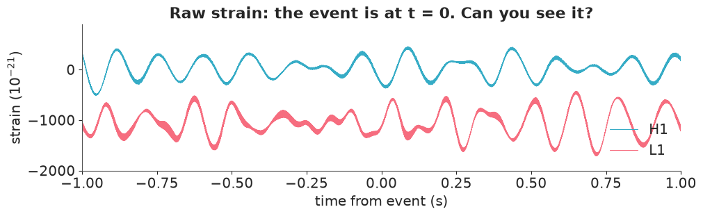
Nothing to see. The raw strain wanders by a few hundred units (L1 also carries a constant offset of about -1000), while the signal we are after peaks at about one unit. The wandering is low-frequency noise (seismic motion, suspension resonances); the detector is only quiet in a band from a few tens to a few hundred hertz. To see anything we must weight each frequency by how noisy it is.
1.2 · The noise spectrum
The power spectral density (PSD) $S(f)$ says how much noise variance there is per hertz. Welch's method estimates it by averaging periodograms of overlapping windowed chunks. We use only off-source data, more than 2 s away from the event, so the signal cannot leak into its own noise estimate.
def offsource_psd(x, times, seconds, guard=2.0):
    """One-sided Welch PSD from data more than `guard` s away from the event (both sides averaged)."""
    rate = 1 / (times[1] - times[0])
    psds, weights = [], []
    for mask in (times < -guard, times > guard):
        freqs_w, p = signal.welch(x[mask], fs=rate, nperseg=int(seconds * rate), window="hann")
        psds.append(p)
        weights.append(mask.sum())
    return freqs_w, np.average(psds, axis=0, weights=weights)


psd = {det: offsource_psd(strain[det], t, seconds=4) for det in DETECTORS}

fig, ax = plt.subplots(figsize=(10, 4))
for det in DETECTORS:
    ax.loglog(psd[det][0], np.sqrt(psd[det][1]), lw=0.8, label=det)
ax.axvspan(35, 350, color="k", alpha=0.07, label="35-350 Hz band")
ax.set(xlim=(10, 2048), ylim=(3e-3, 3e2), xlabel="frequency (Hz)",
       ylabel=r"amplitude spectral density ($10^{-21}/\sqrt{\mathrm{Hz}}$)")
ax.legend();
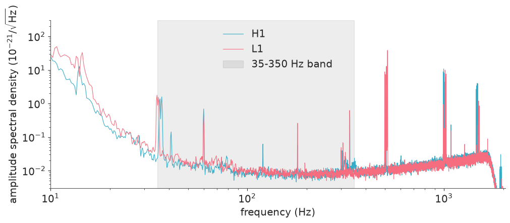
The amplitude spectral density falls by a factor of several thousand - some seven orders of magnitude in power - between 10 Hz and the quiet "bucket" near 100-300 Hz, and there is a forest of narrow lines on top (mains harmonics at multiples of 60 Hz, suspension "violin" modes near 500 Hz and their harmonics near 1 kHz, calibration lines). This is what coloured noise looks like.
1.3 · Whitening and band-passing
Whitening divides the Fourier transform of the data by $\sqrt{S(f)}$. Every frequency then carries the same noise power: the loud low frequencies are turned down, the quiet bucket is turned up. With the normalisation below, stationary Gaussian noise with PSD $S(f)$ becomes (approximately) unit-variance white Gaussian noise. We then band-pass to 35-350 Hz, where the signal lives, using a zero-phase Butterworth response applied in the frequency domain.
freqs = np.fft.rfftfreq(n_samples, dt)
taper = signal.windows.tukey(n_samples, 0.1)  # avoids edge ringing in the FFT
sos_bp = signal.butter(4, [35, 350], btype="bandpass", fs=fs, output="sos")
bp_gain = np.abs(signal.sosfreqz(sos_bp, worN=freqs, fs=fs)[1]) ** 2  # zero-phase, like filtfilt

psd_on_grid = {det: np.interp(freqs, *psd[det]) for det in DETECTORS}
white, white_bp = {}, {}
for det in DETECTORS:
    whitening = 1 / np.sqrt(psd_on_grid[det] * fs / 2)  # white noise of unit variance has S = 2/fs
    spectrum = np.fft.rfft(strain[det] * taper)
    white[det] = np.fft.irfft(spectrum * whitening, n=n_samples)
    white_bp[det] = np.fft.irfft(spectrum * whitening * bp_gain, n=n_samples)

quiet = (np.abs(t) > 2) & (np.abs(t) < 13)
for det in DETECTORS:
    print(f"{det}: off-source std  whitened = {white[det][quiet].std():.2f}   "
          f"whitened + band-passed = {white_bp[det][quiet].std():.2f}")
H1: off-source std  whitened = 0.99   whitened + band-passed = 0.37
L1: off-source std  whitened = 1.15   whitened + band-passed = 0.37
Whitened H1 noise has a standard deviation of 0.99, as designed. L1 comes out at 1.15; the excess sits entirely below 10 Hz (slow drifts that a PSD built from 4 s chunks cannot resolve) and disappears once we band-pass. After the band-pass both detectors are at 0.37: we kept roughly $(350-35)/2048 \approx 15\%$ of the bandwidth and hence of the variance ($\sqrt{0.15} = 0.39$). Hold on to that number - it matters in section 2.8.
Now the famous picture. The source was closer to Livingston, and the two detectors are oriented almost oppositely, so we cross-correlate to find the shift and sign that best overlay L1 on H1.
window = (t > -0.15) & (t < 0.05)
idx = np.flatnonzero(window)
lags = np.arange(-60, 61)  # +-15 ms; the light travel time between the sites is 10 ms
xcorr = np.array([np.sum(white_bp["H1"][idx] * white_bp["L1"][idx - lag]) for lag in lags])
k = np.argmax(np.abs(xcorr))
y0, y1, y2 = np.abs(xcorr[k - 1 : k + 2])
lag_refined = lags[k] + 0.5 * (y0 - y2) / (y0 - 2 * y1 + y2)  # parabolic interpolation of the peak
norm = np.sqrt(np.sum(white_bp["H1"][idx] ** 2) * np.sum(white_bp["L1"][idx - lags[k]] ** 2))

DT_HL = lag_refined * dt  # seconds by which H1 lags L1
SIGN_HL = np.sign(xcorr[k])
print(f"best overlay: shift L1 later by {DT_HL * 1e3:.1f} ms, sign {SIGN_HL:+.0f}, "
      f"correlation {xcorr[k] / norm:.2f}")
best overlay: shift L1 later by 7.3 ms, sign -1, correlation -0.72
T_PEAK = 0.023  # published time of peak strain at Hanford, relative to GPS_EVENT (see section 2.2)

fig, axes = plt.subplots(1, 2, figsize=(12, 3.8), width_ratios=[2, 1])
axes[0].plot(t, white_bp["H1"], label="H1")
axes[0].plot(t + DT_HL, SIGN_HL * white_bp["L1"], label=f"L1, shifted {DT_HL * 1e3:.1f} ms, sign-flipped")
axes[0].set(xlim=(-0.2, 0.08), ylim=(-3.6, 3.6), xlabel="time from event (s)",
            ylabel="whitened strain (noise std)", title="Whitened, band-passed 35-350 Hz")
axes[0].legend(loc="upper left")
axes[1].plot(lags * dt * 1e3, xcorr / norm)
axes[1].axvline(DT_HL * 1e3, color="k", ls=":")
axes[1].set(xlabel="lag of H1 behind L1 (ms)", ylabel="correlation", title="H1-L1 cross-correlation");

envelope = np.abs(signal.hilbert(white_bp["H1"]))
t_env_peak = t[np.argmax(envelope * (np.abs(t) < 0.1))]
print(f"H1 whitened envelope peaks at t = {t_env_peak * 1e3:.1f} ms")
H1 whitened envelope peaks at t = 24.3 ms
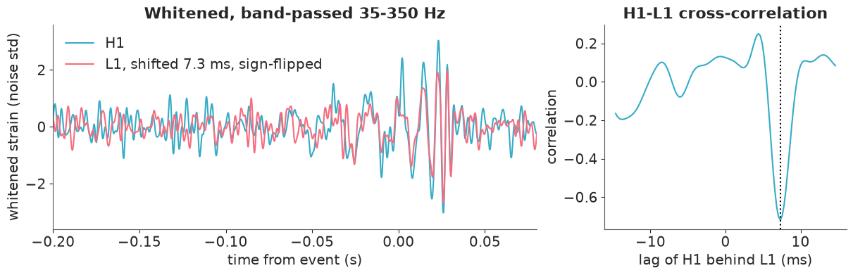
There it is: a handful of cycles growing in amplitude and frequency, a peak, and a rapid decay - the same shape in two instruments 3000 km apart, with Livingston about 7 ms ahead and with the opposite sign (a correlation of -0.72 between two independent detectors). The LIGO papers quote an arrival-time difference of $6.9^{+0.5}_{-0.4}$ ms; our crude cross-correlation estimate of 7.3 ms is in the same place. It is one number from one filter choice with no uncertainty attached; we return to the time shift in 2.5. The correlation has a single clean dip because the chirp is broadband: every frequency agrees on one time shift. Remember that when we get to the narrow-band ringdown.
1.4 · A time-frequency map
A short-time Fourier transform has one fixed time resolution. For a chirp it is better to use windows that get shorter as frequency rises (constant $Q = f/\Delta f$), which is the idea of the "Q-transform" used in LIGO's own plots. A bare-bones version is a Gaussian band-pass around each frequency, applied in the Fourier domain:
def q_transform(x, rate, centre_freqs, q=8.0):
    """Energy in constant-Q Gaussian frequency bands. Each row is normalised by its median."""
    n = len(x)
    spectrum = np.fft.rfft(x)
    fr = np.fft.rfftfreq(n, 1 / rate)
    out = np.empty((len(centre_freqs), n))
    for i, f0 in enumerate(centre_freqs):
        analytic = np.zeros(n, dtype=complex)
        analytic[: len(fr)] = spectrum * np.exp(-0.5 * ((fr - f0) / (f0 / q)) ** 2)  # positive freqs only
        out[i] = np.abs(np.fft.ifft(analytic)) ** 2
    return out / np.median(out, axis=1, keepdims=True)


chunk = np.abs(t) < 2  # transform 4 s so that filter edge effects stay far from the event ...
view = (t[chunk] > -0.3) & (t[chunk] < 0.15)  # ... but draw only what is shown: 8x fewer quads to hold in memory
q_freqs = np.geomspace(25, 500, 120)

fig, axes = plt.subplots(1, 2, figsize=(12, 3.8), sharey=True)
for ax, det in zip(axes, DETECTORS):
    energy = q_transform(white[det][chunk], fs, q_freqs)[:, view]
    mesh = ax.pcolormesh(t[chunk][view], q_freqs, energy, vmin=0, vmax=25, shading="auto", cmap="viridis")
    ax.set(xlim=(-0.25, 0.1), yscale="log", xlabel="time from event (s)", title=det)
    ax.grid(False)
axes[0].set_ylabel("frequency (Hz)")
fig.colorbar(mesh, ax=axes, label="energy / median");
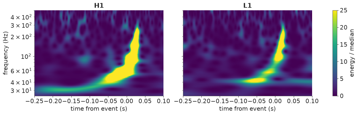
The textbook chirp: the frequency sweeps from about 35 Hz to about 250 Hz in 0.2 s, and the sweep accelerates. In both detectors. That upward sweep is two masses spiralling together (Part 4); the abrupt end is the merger; what follows the peak is the newborn black hole settling down - the ringdown (Part 2).
1.5 · Why whitening gives a likelihood, and where the shortcut breaks
If the noise is stationary and Gaussian, its Fourier coefficients at different frequencies are independent with variance proportional to $S(f)$. That is the Whittle likelihood:
$$\log p(d \mid \theta) = -\tfrac{1}{2}\sum_k \frac{|\tilde d_k - \tilde h_k(\theta)|^2}{\sigma_k^2} + \text{const}, \qquad \sigma_k^2 \propto S(f_k).$$
Dividing by $\sqrt{S}$ makes every $\sigma_k$ equal, and by Parseval's theorem the sum over
frequencies becomes a sum over time samples: whitened data minus whitened template is
unit-variance white noise, i.e. pm.Normal(mu=whitened_template, sigma=1). That is the
attraction. The shortcut has three traps, though:
- The template must be whitened too. The filter changes the shape of any signal. You cannot fit an un-whitened damped sinusoid to whitened data.
- Band-passed samples are not independent. After the band-pass the noise has std 0.37
and neighbouring samples are strongly correlated. If you "helpfully" set or fit
sigma = 0.37with independent samples you count the same information several times. - The filters are acausal and long. Whitening and zero-phase band-passing smear every feature over tens of milliseconds in both directions. For the ringdown we want to use data after a start time $t_0$ and nothing before it - but the filtered data after $t_0$ contain smeared-in power from the much louder merger just before it.
Trap 3 is the reason ringdown analyses in the literature (Isi & Farr 2021, and the
ringdown package) work in the time domain with the full noise covariance matrix.
That is what we will do. It is exact for stationary Gaussian noise, it handles the
truncation at $t_0$ with no leakage, and it whitens data and template with the same
operator by construction. In section 2.8 we come back and measure what the shortcut
would have cost.
Part 2 · The ringdown: weighing a black hole with a damped sinusoid
A perturbed black hole rings like a struck bell, in damped sinusoids called quasi-normal modes. Keeping only the dominant one,
$$h(t) = A\,e^{-(t-t_0)/\tau}\cos\!\big(2\pi f\,(t-t_0) - \varphi\big), \qquad t \ge t_0 .$$
General relativity says $f$ and $\tau$ depend only on the mass and spin of the final black hole, so measuring them weighs the remnant.
2.1 · A noise model in the time domain
Stationary Gaussian noise is fully described by its autocovariance function $\rho(k) = \mathrm{cov}(n_i, n_{i+k})$, the inverse Fourier transform of the PSD. For a window of $N$ samples the noise is $\mathcal{N}(0, C)$ with $C_{ij} = \rho(|i-j|)$. With the Cholesky factor $C = LL^\top$,
$$ L^{-1} d \;\sim\; \mathcal{N}\big(L^{-1} h(\theta),\; I\big). $$
$L^{-1}$ is a whitening filter too - the time-domain, finite-window counterpart of dividing by $\sqrt{S(f)}$ - but it is lower-triangular, hence causal: nothing before the window leaks in, and the template is whitened by the same matrix as the data.
Conditioning, following common practice: high-pass at 20 Hz (below that there is only noise, and it would wreck the conditioning of $C$), down-sample to 2048 Hz (the ringdown is at ~250 Hz; the top octave only adds cost and an anti-aliasing roll-off that $C$ would have to model), then estimate the PSD from off-source data as before.
t_fit = t[::2]
FS_FIT = fs / 2
sos_hp = signal.butter(4, 20, btype="highpass", fs=fs, output="sos")
cond = {det: signal.decimate(signal.sosfiltfilt(sos_hp, strain[det]), 2, ftype="fir", zero_phase=True)
        for det in DETECTORS}

# autocovariance = inverse FFT of the one-sided PSD; the factor turns a density into a variance
acf = {det: 0.5 * FS_FIT * np.fft.irfft(offsource_psd(cond[det], t_fit, seconds=2)[1]) for det in DETECTORS}


def whitener(det, n):
    """L^-1 for an n-sample window: maps noise with this detector's covariance to N(0, I)."""
    chol = np.linalg.cholesky(linalg.toeplitz(acf[det][:n]))
    return linalg.solve_triangular(chol, np.eye(n), lower=True)


N_RING = 102  # 50 ms at 2048 Hz: a dozen damping times
W_RING = {det: whitener(det, N_RING) for det in DETECTORS}
Test the noise model on noise before trusting it with a signal. Whitening non-overlapping off-source windows should give independent standard-normal numbers. (The same data informed the PSD, so the overall variance is nearly 1 by construction; the absence of correlation and the Gaussian shape are the non-trivial checks.)
starts = np.arange(200, len(t_fit) - N_RING - 200, N_RING)
starts = starts[np.abs(t_fit[starts]) > 2]

fig, axes = plt.subplots(1, 2, figsize=(11, 3.5))
grid = np.linspace(-4.5, 4.5, 200)
for det in DETECTORS:
    raw = np.array([cond[det][s : s + N_RING] for s in starts])
    z = raw @ W_RING[det].T
    lag1 = np.mean(z[:, 1:] * z[:, :-1])
    lag1_raw = np.mean(raw[:, 1:] * raw[:, :-1]) / raw.var()
    print(f"{det}: {len(starts)} windows   mean square = {np.mean(z**2):.3f}   lag-1 correlation: "
          f"before {lag1_raw:+.3f}, after {lag1:+.3f}   excess kurtosis = {stats.kurtosis(z.ravel()):+.3f}")
    axes[0].plot(np.arange(60) / FS_FIT * 1e3, acf[det][:60] / acf[det][0], label=det)
    axes[1].hist(z.ravel(), bins=80, density=True, histtype="step", label=f"{det} whitened")
axes[0].set(xlabel="lag (ms)", ylabel="autocorrelation", title="Conditioned noise: dominated by ringing lines")
axes[0].legend()
axes[1].plot(grid, stats.norm.pdf(grid), "k--", lw=1, label="N(0, 1)")
axes[1].set(xlabel="whitened sample", yscale="log", ylim=(1e-5, 1), title="...and white and Gaussian after $L^{-1}$")
axes[1].legend();
H1: 558 windows   mean square = 0.996   lag-1 correlation: before -0.933, after -0.001   excess kurtosis = -0.028
L1: 558 windows   mean square = 0.995   lag-1 correlation: before -0.033, after +0.001   excess kurtosis = -0.029
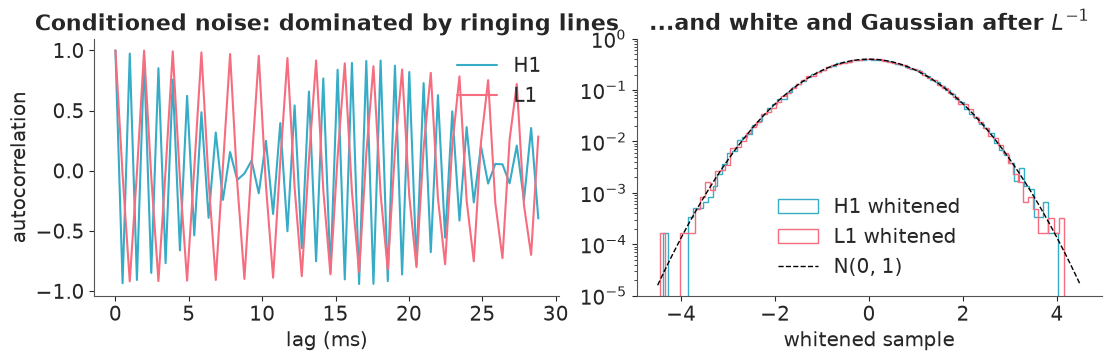
The conditioned noise is as far from white as it gets. Once the low frequencies are removed, about 96% of the remaining variance is in narrow lines - near 1 kHz in H1, just below the new Nyquist frequency, which is why its neighbouring samples are anti-correlated at -0.93; near 515 Hz in L1 - and lines ring for a long time. After $L^{-1}$ all of that is gone: the lag-1 correlation is zero to three decimals, the variance is 1, and the tails follow the Gaussian over four decades. For these 30 seconds, "stationary and Gaussian" is a good description.
2.2 · The model
Phase as quadratures. Writing $A\cos(\omega t - \varphi) = a_c\cos\omega t + a_s\sin\omega t$ with $a_c = A\cos\varphi,\ a_s = A\sin\varphi$ replaces a wrapped angle by two unbounded numbers. NUTS moves through a Euclidean space: it cannot step from $\varphi = 3.1$ to $-3.1$ even though they are neighbours on the circle, so a posterior that straddles the wrap looks bimodal to it, and at $A \to 0$ the phase is undefined (a funnel). In quadratures the posterior is a single blob - and, given $(f, \tau)$, the template is linear in $(a_c, a_s)$ with Gaussian priors, which we will exploit in Part 3. Independent $\mathcal{N}(0, s)$ priors on the quadratures imply a uniform phase and a Rayleigh amplitude.
Two detectors. Each detector gets its own quadratures. Why not "one amplitude and phase, plus a time shift and a relative amplitude"? Because for a damped sinusoid a time shift $\delta$ is a phase shift $2\pi f\delta$ and a rescaling $e^{\delta/\tau}$: the two parameterisations describe the same family of curves, but the time-shift version has a ridge that repeats every $1/f \approx 4$ ms. So we align the L1 window using the cross-correlation shift from Part 1, keep the well-behaved parameters, and derive the relative amplitude, the sign and the implied time shift afterwards (2.5).
Start time. The model only holds once the remnant has settled into linear ringing.
Published analyses put the peak strain at Hanford at about GPS 1126259462.423 (T_PEAK,
t = 23 ms here; our whitened envelope peaks 1-2 ms later, which is within the smearing of
the filters). Guided by the LIGO-Virgo testing-GR paper, where a single damped sinusoid
starts to agree with the full analysis about 3 ms after the merger, we start 3 ms after
the peak, and treat that as a choice to be stress-tested (2.6), not a fact. Start times are
rounded up to the next sample (at most 0.5 ms).
Priors. $f \sim \text{Uniform}(150, 400)$ Hz: the ringdown should sit at or above the ~150-250 Hz reached at the end of the chirp in the time-frequency map. $\tau \sim \text{LogNormal}(\log 4\text{ ms}, 0.75)$, i.e. roughly 1-17 ms: a bell that rings for a handful of cycles. Quadratures $\sim \mathcal{N}(0, 2)$ in units of $10^{-21}$, because the published peak strain is about 1 in those units.
AMP_SD = 2.0
MSUN_S = 4.925491e-6  # G * Msun / c^3 in seconds: a solar mass expressed as a time

# Berti-Cardoso-Will (2006) fits for the l = m = 2, n = 0 Kerr quasi-normal mode
F1, F2, F3 = 1.5251, -1.1568, 0.1292
Q1, Q2, Q3 = 0.7000, 1.4187, -0.4990


def ringdown_parts(t0_h1, n=N_RING):
    """Per detector: time since the first sample at or after t0, whitening matrix, whitened data, start."""
    parts = {}
    for det in DETECTORS:
        i = np.searchsorted(t_fit, t0_h1 - (DT_HL if det == "L1" else 0.0))
        parts[det] = (np.arange(n) / FS_FIT, W_RING[det], W_RING[det] @ cond[det][i : i + n], t_fit[i])
    return parts


def ringdown_model(parts, kerr_prior=False, sigma=1.0):
    with pm.Model(coords={"det": DETECTORS}) as model:
        if kerr_prior:  # section 2.7
            mass = pm.Uniform("mass", 35, 140)
            chi = pm.Uniform("chi", 0, 0.99)
            f = pm.Deterministic("f", (F1 + F2 * (1 - chi) ** F3) / (2 * np.pi * mass * MSUN_S))
            tau_ms = pm.Deterministic("tau_ms", 1e3 * (Q1 + Q2 * (1 - chi) ** Q3) / (np.pi * f))
        else:
            f = pm.Uniform("f", 150, 400)
            tau_ms = pm.LogNormal("tau_ms", np.log(4), 0.75)
        a_cos = pm.Normal("a_cos", 0, AMP_SD, dims="det")
        a_sin = pm.Normal("a_sin", 0, AMP_SD, dims="det")

        snr_sq = 0
        for k, det in enumerate(DETECTORS):
            tw, W, y, _ = parts[det]
            h = pt.exp(-tw / (tau_ms / 1e3)) * (
                a_cos[k] * pt.cos(2 * np.pi * f * tw) + a_sin[k] * pt.sin(2 * np.pi * f * tw)
            )
            h_white = pt.dot(W, h)  # the template goes through the same whitening as the data
            pm.Normal(f"y_{det}", mu=h_white, sigma=sigma, observed=y)
            snr_sq += pt.sum(h_white**2) / sigma**2

        pm.Deterministic("amp", pt.sqrt(a_cos**2 + a_sin**2), dims="det")
        pm.Deterministic("snr", pt.sqrt(snr_sq))  # network "optimal" signal-to-noise ratio of the template
    return model


T0_OFFSET = 0.003
ring_parts = ringdown_parts(T_PEAK + T0_OFFSET)
ring_model = ringdown_model(ring_parts)
ring_model
2.3 · Prior predictive check
The derived snr is $\lVert L^{-1}h\rVert$ summed over detectors: how many noise standard
deviations the template stands out by. It is the natural scale on which to ask what the
priors claim.
with ring_model:
    ring_prior = pm.sample_prior_predictive(1000, random_seed=RANDOM_SEED)


def ringdown_np(tw, f, tau_ms, a_cos, a_sin):
    return np.exp(-tw / (tau_ms / 1e3)) * (a_cos * np.cos(2 * np.pi * f * tw) + a_sin * np.sin(2 * np.pi * f * tw))


prior = az.extract(ring_prior, group="prior", num_samples=40, random_seed=RANDOM_SEED)
tw = np.arange(N_RING) / FS_FIT

fig, axes = plt.subplots(1, 2, figsize=(11, 3.5))
for j in range(prior.sizes["sample"]):
    p = prior.isel(sample=j)
    axes[0].plot(tw * 1e3, ringdown_np(tw, float(p["f"]), float(p["tau_ms"]), *p["a_cos"].values[:1], *p["a_sin"].values[:1]),
                 color="C0", alpha=0.35)
axes[0].set(xlim=(0, 30), xlabel="time since $t_0$ (ms)", ylabel="strain ($10^{-21}$)", title="Prior draws of the H1 ringdown")
prior_snr = ring_prior.prior["snr"].values.ravel()
axes[1].hist(np.log10(prior_snr), bins=40)
axes[1].set(xlabel="log10 prior SNR", title="Implied signal-to-noise ratio")
print("prior SNR quantiles (5%, 50%, 95%):", np.quantile(prior_snr, [0.05, 0.5, 0.95]).round(1))
prior SNR quantiles (5%, 50%, 95%): [ 5.5 15.2 37.6]
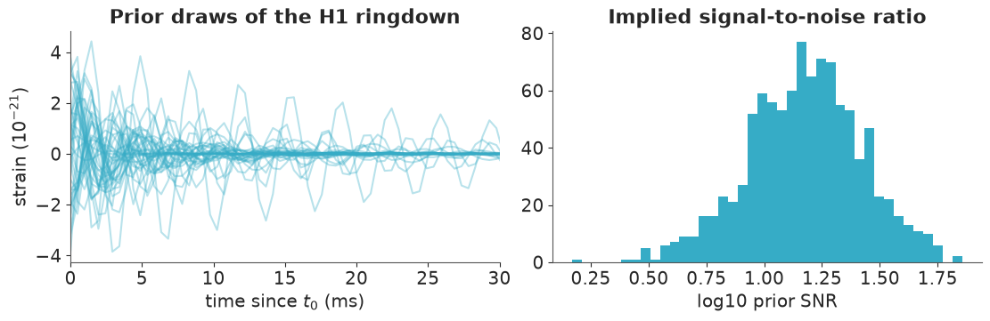
Damped wiggles of a few cycles with amplitudes of a few units: the right kind of object. The implied SNR runs from about 5 (marginal) to about 40 (unmissable), with a median of 15. So this prior leans towards signals that are louder than a ringdown 3 ms after the peak is likely to be - acceptable as a weakly-informative choice, but worth knowing; in Part 3 we will see how much the Bayes factor cares.
2.4 · Fit, diagnose, check
with ring_model:
    ring_idata = pm.sample(random_seed=RANDOM_SEED)

print("divergences:", int(ring_idata.sample_stats["diverging"].sum()))
az.summary(ring_idata, var_names=["f", "tau_ms", "amp", "snr"], ci_kind="hdi", ci_prob=0.9, round_to=2)
divergences: 0
| mean | sd | hdi90_lb | hdi90_ub | ess_bulk | ess_tail | r_hat | mcse_mean | mcse_sd | |
|---|---|---|---|---|---|---|---|---|---|
| f | 246.97 | 12.46 | 227.98 | 265.14 | 1204.04 | 1441.03 | 1.00 | 0.39 | 0.62 |
| tau_ms | 4.50 | 1.19 | 2.74 | 6.46 | 1299.43 | 1731.15 | 1.01 | 0.03 | 0.03 |
| amp[H1] | 1.23 | 0.26 | 0.81 | 1.64 | 1823.29 | 2350.26 | 1.00 | 0.01 | 0.00 |
| amp[L1] | 1.00 | 0.25 | 0.59 | 1.38 | 1728.81 | 2230.69 | 1.00 | 0.01 | 0.00 |
| snr | 8.03 | 1.02 | 6.47 | 9.77 | 4733.01 | 3289.68 | 1.00 | 0.01 | 0.01 |
az.plot_trace_dist(ring_idata, var_names=["f", "tau_ms", "a_cos", "a_sin"]);
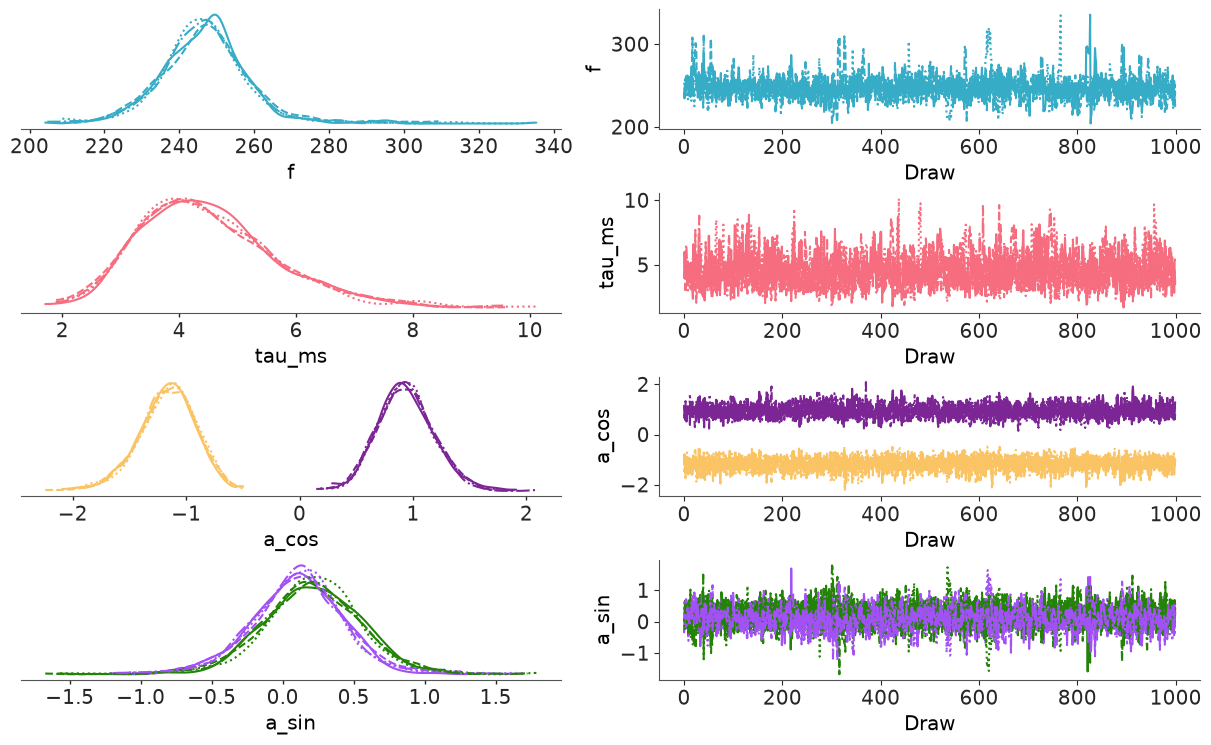
Clean: no divergences, r_hat at most 1.01, ESS above a thousand. Six parameters, 204 data
points and a 102 x 102 matrix product per gradient - the whole fit takes a few seconds.
For the posterior predictive check we look at the data the way the likelihood sees them: whitened by $L^{-1}$. If the model is adequate, whitened data minus whitened template should be standard normal noise.
post = az.extract(ring_idata, num_samples=500, random_seed=RANDOM_SEED)

fig, axes = plt.subplots(1, 2, figsize=(12, 3.6), sharey=True)
for k, (ax, det) in enumerate(zip(axes, DETECTORS)):
    tw, W, y, _ = ring_parts[det]
    templates = np.array([
        W @ ringdown_np(tw, f_, tau_, ac_, as_)
        for f_, tau_, ac_, as_ in zip(post["f"].values, post["tau_ms"].values,
                                      post["a_cos"].values[k], post["a_sin"].values[k])
    ])
    lo, hi = np.quantile(templates, [0.05, 0.95], axis=0)
    ax.plot(tw * 1e3, y, "k.-", lw=0.6, ms=3, label="whitened data $L^{-1}d$")
    ax.fill_between(tw * 1e3, lo, hi, color=f"C{k}", alpha=0.5, label="whitened template, 90% band")
    ax.set(xlim=(0, 30), xlabel="time since $t_0$ (ms)", title=det)
    ax.legend(loc="upper right")
    resid = y - templates
    print(f"{det}: mean square of whitened data = {np.mean(y**2):.2f}, "
          f"of whitened residuals = {np.mean(resid**2, axis=1).mean():.2f} (expect about 1)")
axes[0].set_ylabel("noise standard deviations");
H1: mean square of whitened data = 1.40, of whitened residuals = 1.04 (expect about 1)
L1: mean square of whitened data = 1.06, of whitened residuals = 0.84 (expect about 1)
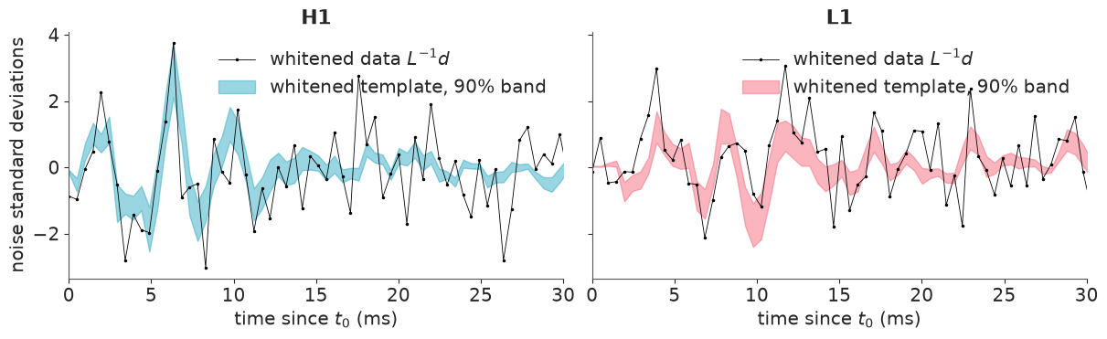
The whitened template is not a pretty damped sinusoid - $L^{-1}$ reshapes it, which is exactly why the template must go through the same operator as the data. The first few samples carry the signal (several standard deviations), and after subtracting the template the residual mean square is compatible with 1 (for 102 samples it scatters by about 0.14; in H1 it drops from 1.40 to 1.04). A ringdown starting 3 ms after the peak is a weak signal: a network SNR of about 8, spread over a handful of samples.
2.5 · Do the two detectors tell the same story?
Each detector has its own amplitude and phase. If both see the same wave, with Livingston inverted and ahead by $\Delta t$, then after our alignment the phases should differ by $\pi$, and any leftover phase is a leftover time shift: $\Delta t = \Delta t_\text{used} - (\Delta\varphi - \pi)/(2\pi f)$.
p = ring_idata.posterior
phase = np.arctan2(p["a_sin"], p["a_cos"])
dphi = (phase.sel(det="L1") - phase.sel(det="H1")) % (2 * np.pi)
dt_used = ring_parts["H1"][3] - ring_parts["L1"][3]
dt_implied = 1e3 * (dt_used - (dphi - np.pi) / (2 * np.pi * p["f"]))
amp_ratio = p["amp"].sel(det="L1") / p["amp"].sel(det="H1")

for label, x in [("phase difference / pi", dphi / np.pi), ("implied H1-L1 time shift (ms)", dt_implied),
                 ("amplitude ratio L1/H1", amp_ratio)]:
    q = np.quantile(x, [0.05, 0.5, 0.95])
    print(f"{label:<32} median {q[1]:.2f}   90% interval [{q[0]:.2f}, {q[2]:.2f}]")
phase difference / pi            median 1.09   90% interval [0.94, 1.25]
implied H1-L1 time shift (ms)    median 7.13   90% interval [6.82, 7.45]
amplitude ratio L1/H1            median 0.81   90% interval [0.51, 1.23]
The phase difference is compatible with $\pi$ - the sign flip; you can also see it in the
trace plot above, where a_cos is about -1.1 in H1 and +0.9 in L1. Read as a time shift,
the ringdown alone gives 7.1 ms with a 90% interval of 6.8-7.5 ms, overlapping both the
cross-correlation value and the published $6.9^{+0.5}_{-0.4}$ ms. Two caveats: this is the
solution nearest to the alignment we imposed (add any multiple of $1/f \approx 4$ ms and
the fit is identical - the interval is conditional on having picked the right cycle), and
"same wave, inverted" is only approximately true because the detectors are not exactly
anti-aligned. The amplitude ratio is compatible with 1 and poorly measured.
2.6 · The start time is a modelling choice - so vary it
Start too early and the data still contain the non-linear merger, which a single damped sinusoid cannot describe (bias). Start too late and the signal has decayed into the noise (variance). There is no objectively correct $t_0$, so we show the dependence.
offsets_ms = [0, 1, 3, 5, 7]
scan = {}
for off in offsets_ms:
    if off == 1e3 * T0_OFFSET:
        scan[off] = ring_idata
        continue
    with ringdown_model(ringdown_parts(T_PEAK + off / 1e3)):
        scan[off] = pm.sample(random_seed=RANDOM_SEED, progressbar=False)

rows = []
for off, idata in scan.items():
    row = {"t0 - t_peak (ms)": off}
    for v in ["f", "tau_ms", "snr"]:
        lo, med, hi = np.quantile(idata.posterior[v], [0.05, 0.5, 0.95])
        row.update({f"{v} median": med, f"{v} lo": lo, f"{v} hi": hi})
    row["max r_hat"] = float(az.summary(idata, var_names=["f", "tau_ms", "a_cos", "a_sin"])["r_hat"].max())
    row["divergences"] = int(idata.sample_stats["diverging"].sum())
    rows.append(row)
scan_table = pd.DataFrame(rows).set_index("t0 - t_peak (ms)")
scan_table.round(2)
| f median | f lo | f hi | tau_ms median | tau_ms lo | tau_ms hi | snr median | snr lo | snr hi | max r_hat | divergences | |
|---|---|---|---|---|---|---|---|---|---|---|---|
| t0 - t_peak (ms) | |||||||||||
| 0 | 234.13 | 223.84 | 242.49 | 5.50 | 4.22 | 7.13 | 12.33 | 10.74 | 13.98 | 1.00 | 0 |
| 1 | 233.41 | 218.94 | 244.48 | 5.38 | 3.82 | 7.60 | 9.73 | 8.10 | 11.36 | 1.01 | 0 |
| 3 | 246.74 | 228.16 | 265.57 | 4.34 | 2.86 | 6.70 | 8.03 | 6.40 | 9.73 | 1.01 | 0 |
| 5 | 278.31 | 210.33 | 358.93 | 2.29 | 1.14 | 4.93 | 5.60 | 3.96 | 7.16 | 1.01 | 0 |
| 7 | 218.47 | 155.89 | 362.48 | 1.13 | 0.46 | 2.71 | 3.84 | 2.34 | 5.36 | 1.01 | 0 |
def kerr_qnm(mass, chi):
    """Frequency (Hz) and damping time (s) of the 220 mode of a Kerr black hole (mass in Msun, detector frame)."""
    f = (F1 + F2 * (1 - chi) ** F3) / (2 * np.pi * mass * MSUN_S)
    return f, (Q1 + Q2 * (1 - chi) ** Q3) / (np.pi * f)


f_pub, tau_pub = kerr_qnm(68.0, 0.69)
print(f"Kerr black hole with M = 68 Msun, chi = 0.69:  f = {f_pub:.0f} Hz, tau = {tau_pub * 1e3:.2f} ms")

fig, axes = plt.subplots(1, 3, figsize=(13, 3.6))
for ax, v, ref, label in zip(axes, ["f", "tau_ms", "snr"], [f_pub, tau_pub * 1e3, None],
                             ["f (Hz)", r"$\tau$ (ms)", "SNR of the fitted ringdown"]):
    med, lo, hi = (scan_table[f"{v} {c}"] for c in ["median", "lo", "hi"])
    ax.errorbar(scan_table.index, med, yerr=[med - lo, hi - med], fmt="o", capsize=3)
    if ref is not None:
        ax.axhline(ref, color="k", ls="--", lw=1, label="Kerr mode of the\npublished remnant")
    if v == "f":
        ax.legend(loc="lower left")
    ax.set(xlabel="$t_0 - t_{peak}$ (ms)", ylabel=label)
fig.suptitle("Ringdown posterior (median, 90% interval) against the start time");
Kerr black hole with M = 68 Msun, chi = 0.69: f = 252 Hz, tau = 4.10 ms
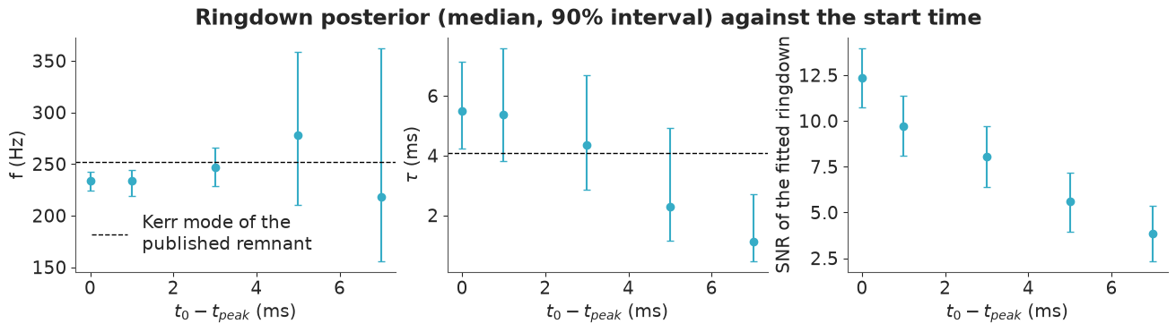
Read the three panels together:
- SNR falls steadily as we start later - the signal decays with a ~4 ms time constant.
- At 0-1 ms the posterior is narrow but sits at a lower frequency (233-234 Hz) and a longer damping time (about 5.5 ms) than the Kerr mode of the published remnant. Precise and biased: a single mode is being asked to describe the merger. (Published work argues that adding overtones repairs this; see "Try it yourself".)
- At 3 ms the posterior is centred near 247 Hz and 4.3 ms, and comfortably contains the expected mode. The LIGO-Virgo testing-GR paper reports the same qualitative pattern: its damped-sinusoid fit becomes consistent with the full-waveform prediction from about 3 ms after the merger.
- By 5-7 ms the posterior for $f$ spreads over much of its prior and $\tau$ drifts
towards short values: there is little signal left, and what the fit finds is
increasingly noise. Notice the
snrpanel cannot tell you that by itself - a flexible template always finds something (Part 3).
The dashed reference line was computed with the fitting formulas we meet next, so let us do that properly.
2.7 · The payoff: mass and spin of the remnant
For a Kerr black hole of mass $M$ and dimensionless spin $\chi$, Berti, Cardoso & Will (2006) give accurate fits for the dominant ($\ell = m = 2$, $n = 0$) mode:
$$2\pi f\,\frac{GM}{c^3} = f_1 + f_2(1-\chi)^{f_3}, \qquad Q \equiv \pi f\tau = q_1 + q_2(1-\chi)^{q_3}.$$
The quality factor $Q$ depends on spin only; given the spin, the frequency sets the mass. The check above (68 $M_\odot$, $\chi = 0.69$ gives 252 Hz and 4.1 ms) is our sanity test of the constants and units. Inverting is one line per draw - but it is only possible when $Q > q_1 + q_2 = 2.12$ (the value at $\chi = 0$). Draws with a lower $Q$ ring down faster than any Kerr black hole would, and have no mass or spin.
def invert_kerr(f, tau):
    quality = np.pi * f * tau
    with np.errstate(invalid="ignore"):
        chi = 1 - ((quality - Q1) / Q2) ** (1 / Q3)
        mass = (F1 + F2 * (1 - chi) ** F3) / (2 * np.pi * f * MSUN_S)
    return mass, chi


draws = az.extract(ring_idata, var_names=["f", "tau_ms"])
mass_draws, chi_draws = invert_kerr(draws["f"].values, draws["tau_ms"].values / 1e3)
physical = np.isfinite(chi_draws) & (chi_draws >= 0)
print(f"share of posterior draws with no Kerr counterpart (Q < 2.12): {1 - physical.mean():.1%}")
for label, x in [("mass (Msun, detector frame)", mass_draws[physical]), ("spin chi", chi_draws[physical])]:
    q = np.quantile(x, [0.05, 0.5, 0.95])
    print(f"{label:<30} median {q[1]:.2f}   90% interval [{q[0]:.2f}, {q[2]:.2f}]")
share of posterior draws with no Kerr counterpart (Q < 2.12): 3.7%
mass (Msun, detector frame)    median 71.49   90% interval [54.57, 87.60]
spin chi                       median 0.73   90% interval [0.26, 0.90]
A few percent of the draws are "not a Kerr black hole". That is a symptom of a prior that was flat in $(f, \tau)$ and knew nothing about black holes. If we believe the remnant is a Kerr black hole, the honest thing is to put the prior where the belief is: sample $M$ and $\chi$ directly and compute $(f, \tau)$ from them inside the model. With a likelihood this weak, the two priors will not give the same answer - that is the point of doing both.
with ringdown_model(ring_parts, kerr_prior=True):
    kerr_idata = pm.sample(random_seed=RANDOM_SEED)

print("divergences:", int(kerr_idata.sample_stats["diverging"].sum()))
az.summary(kerr_idata, var_names=["mass", "chi", "f", "tau_ms"], ci_kind="eti", ci_prob=0.9, round_to=2)
divergences: 0
| mean | sd | eti90_lb | eti90_ub | ess_bulk | ess_tail | r_hat | mcse_mean | mcse_sd | |
|---|---|---|---|---|---|---|---|---|---|
| mass | 67.82 | 10.50 | 51.86 | 85.47 | 388.16 | 554.85 | 1.01 | 0.54 | 0.33 |
| chi | 0.59 | 0.22 | 0.16 | 0.89 | 405.35 | 552.07 | 1.01 | 0.01 | 0.01 |
| f | 245.52 | 12.19 | 226.96 | 265.78 | 1893.12 | 1752.33 | 1.00 | 0.29 | 0.33 |
| tau_ms | 4.22 | 1.20 | 2.92 | 6.33 | 390.08 | 552.03 | 1.01 | 0.06 | 0.12 |
No divergences and r_hat at 1.00-1.01, but the ESS for mass and spin is a few hundred
rather than a thousand-plus: the curved mass-spin ridge below is harder going for NUTS
than the blob in $(f, \tau)$. Adequate for the 90% intervals we quote; run longer before
quoting anything finer.
kerr_draws = az.extract(kerr_idata, var_names=["mass", "chi"])
sub = rng.choice(np.flatnonzero(physical), 1500, replace=False)

fig, axes = plt.subplots(1, 2, figsize=(12, 4.2))
axes[0].scatter(draws["f"].values, draws["tau_ms"].values, s=4, alpha=0.3)
f_line, tau_line = kerr_qnm(np.linspace(40, 140, 50), 0.0)
axes[0].plot(f_line, tau_line * 1e3, color="C3", lw=2, label=r"Kerr with $\chi = 0$: nothing physical below")
axes[0].plot(f_pub, tau_pub * 1e3, "w*", ms=16, mec="k", label="published remnant")
axes[0].set(xlim=(190, 320), ylim=(0, 12), xlabel="f (Hz)", ylabel=r"$\tau$ (ms)", title=r"Posterior of (f, $\tau$)")
axes[0].legend(loc="upper right")

axes[1].scatter(mass_draws[sub], chi_draws[sub], s=4, alpha=0.3)
axes[1].scatter(kerr_draws["mass"].values[:1500], kerr_draws["chi"].values[:1500], s=4, alpha=0.3)
axes[1].scatter([], [], s=30, color="C0", label=r"flat prior in (f, $\tau$), mapped")  # legible legend entries
axes[1].scatter([], [], s=30, color="C1", label=r"flat prior in (M, $\chi$)")
axes[1].plot(68, 0.68, "w*", ms=16, mec="k", label="published (approx.)")
axes[1].set(xlim=(35, 120), ylim=(0, 1), xlabel=r"remnant mass ($M_\odot$, detector frame)", ylabel=r"spin $\chi$",
            title="Mass and spin of the remnant")
axes[1].legend(loc="lower right");
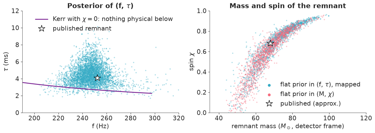
From 50 milliseconds of data and a damped sinusoid: a black hole of very roughly 70 solar masses, spinning at some large fraction of the maximum. The published values from the full analysis are a detector-frame mass of about 68 $M_\odot$ (62-63 $M_\odot$ in the source frame, after removing the cosmological redshift $z \approx 0.09$ - a ringdown alone cannot do that, it only ever measures the redshifted mass) and a spin of 0.67-0.69. Those sit well inside our posterior. But be clear about how little that says:
- Our 90% intervals are broad - roughly 52-88 $M_\odot$, and a spin anywhere from 0.15 to 0.9 depending on the prior. Almost all of the published precision comes from the inspiral and merger, which we threw away. Broad is the correct answer for a ringdown-only analysis at this SNR.
- Mass and spin are strongly correlated (the banana in the right panel): a heavier, faster-spinning hole rings at the same frequency as a lighter, slower one.
- The answer depends on the prior: the flat-in-$(M,\chi)$ fit prefers a lower spin (about 0.6) than the mapped flat-in-$(f,\tau)$ fit (about 0.7), because equal areas in $(f,\tau)$ are not equal areas in $(M,\chi)$ - high spins occupy a large slice of $\tau$. Neither is "the" answer; reporting both is more honest than reporting one.
- And it depends on $t_0$ (2.6).
2.8 · What would the whitening shortcut have cost?
Back to section 1.5. Suppose we had fitted the Part 1 data - FFT-whitened, band-passed, at
4096 Hz - with independent Normal errors, from the same $t_0$. To be fair to the
shortcut we whiten the template correctly: the combined whitening + band-pass filter is a
convolution, so on a window it is a matrix built from its impulse response, and the very
same PyMC model applies with a different W. We try two noise levels: sigma = 1
(the level before band-passing, which is what Parseval's theorem justifies) and
sigma = 0.37 (the measured std of the band-passed noise, which is what most of us
would reach for).
N_SHORT = 205  # the same 50 ms, at 4096 Hz


def shortcut_parts(t0_h1):
    parts = {}
    lag_idx = np.arange(N_SHORT)[:, None] - np.arange(N_SHORT)[None, :]
    for det in DETECTORS:
        kernel = np.fft.irfft(bp_gain / np.sqrt(psd_on_grid[det] * fs / 2), n=n_samples)  # impulse response
        i = np.searchsorted(t, t0_h1 - (DT_HL if det == "L1" else 0.0))
        parts[det] = (np.arange(N_SHORT) / fs, kernel[lag_idx % n_samples], white_bp[det][i : i + N_SHORT], t[i])
    return parts


sigma_bp = np.mean([white_bp[det][quiet].std() for det in DETECTORS])
fits = {"exact: time-domain covariance": ring_idata}
for label, sigma in [("shortcut, sigma = 1", 1.0), (f"shortcut, sigma = {sigma_bp:.2f}", sigma_bp)]:
    with ringdown_model(shortcut_parts(T_PEAK + T0_OFFSET), sigma=sigma):
        fits[label] = pm.sample(random_seed=RANDOM_SEED, progressbar=False)

comparison = pd.concat(
    {label: az.summary(idata, var_names=["f", "tau_ms", "amp"], round_to=4)[["mean", "sd", "r_hat"]]
     for label, idata in fits.items()}
).round(2)
comparison
| mean | sd | r_hat | ||
|---|---|---|---|---|
| exact: time-domain covariance | f | 246.97 | 12.46 | 1.00 |
| tau_ms | 4.50 | 1.19 | 1.01 | |
| amp[H1] | 1.23 | 0.26 | 1.00 | |
| amp[L1] | 1.00 | 0.25 | 1.00 | |
| shortcut, sigma = 1 | f | 244.30 | 13.73 | 1.00 |
| tau_ms | 2.85 | 0.71 | 1.01 | |
| amp[H1] | 2.00 | 0.44 | 1.00 | |
| amp[L1] | 1.85 | 0.46 | 1.00 | |
| shortcut, sigma = 0.37 | f | 243.34 | 3.75 | 1.00 |
| tau_ms | 3.13 | 0.31 | 1.00 | |
| amp[H1] | 1.83 | 0.15 | 1.00 | |
| amp[L1] | 1.69 | 0.16 | 1.00 |
Two different failures, neatly separated:
sigma = 0.37shrinks the posterior standard deviations by a factor of two to four relative tosigma = 1(just under 3 for the amplitudes, which scale withsigma). Nothing about the data improved; we told the model that 205 strongly correlated samples were independent measurements at the band-passed noise level. The rule of thumb: band-limited noise of bandwidth $B$ has only $2B$ independent samples per second (here 630, not 4096), so the information is over-counted by $4096/630 \approx 6.5$ and widths shrink by about $\sqrt{6.5} \approx 2.5$ - the same ballpark. Overconfident by a factor of three is the kind of error that produces false "tensions" with general relativity.sigma = 1gives sensible widths, as the Parseval argument promised, but the answer has moved: a damping time under 3 ms instead of 4.5 ms, and amplitudes more than half as large again as in the exact fit. The likely culprit is trap 3: the acausal filters smear the loud merger into the first milliseconds after $t_0$, and the model explains that extra power with a bigger, faster-decaying ringdown. We have not proven that here (an injection study would), but it is the reason the ringdown literature gives for working in the time domain.
So the exact time-domain likelihood is not pedantry. It is also no harder to write.
Part 3 · Is there really a signal?
A damped sinusoid with free frequency, decay, amplitude and phase will fit something in any stretch of noise. Before believing Part 2 we should ask how the same analysis behaves when there is nothing there - and we have 30 seconds of "nothing there" in the same file.
3.1 · The same model on off-source data
off_times = [-11.0, -7.0, -3.0, 4.0, 8.0, 12.0]
rows = [{"segment": "on-source", "snr": ring_idata.posterior["snr"], "idata": ring_idata}]
for t_off in off_times:
    with ringdown_model(ringdown_parts(t_off)):
        idata = pm.sample(random_seed=RANDOM_SEED, progressbar=False)
    rows.append({"segment": f"t = {t_off:+.0f} s", "snr": idata.posterior["snr"], "idata": idata})

off_table = pd.DataFrame([
    {"segment": r["segment"],
     "snr median": float(r["snr"].median()),
     "snr 5%": float(r["snr"].quantile(0.05)), "snr 95%": float(r["snr"].quantile(0.95)),
     "amp H1 median": float(r["idata"].posterior["amp"].sel(det="H1").median()),
     "f sd (Hz)": float(r["idata"].posterior["f"].std()),
     "max r_hat": float(az.summary(r["idata"], var_names=["f", "tau_ms", "a_cos", "a_sin"])["r_hat"].max()),
     "divergences": int(r["idata"].sample_stats["diverging"].sum())}
    for r in rows
]).set_index("segment")
off_table.round(2)
| snr median | snr 5% | snr 95% | amp H1 median | f sd (Hz) | max r_hat | divergences | |
|---|---|---|---|---|---|---|---|
| segment | |||||||
| on-source | 8.03 | 6.40 | 9.73 | 1.21 | 12.46 | 1.01 | 0 |
| t = -11 s | 2.29 | 1.06 | 3.77 | 0.69 | 71.40 | 1.01 | 5 |
| t = -7 s | 2.14 | 1.00 | 3.57 | 0.55 | 80.53 | 1.00 | 1 |
| t = -3 s | 2.93 | 1.59 | 4.49 | 0.74 | 67.32 | 1.03 | 11 |
| t = +4 s | 2.69 | 1.34 | 4.14 | 1.02 | 74.84 | 1.00 | 1 |
| t = +8 s | 3.62 | 2.15 | 5.23 | 1.04 | 78.41 | 1.00 | 0 |
| t = +12 s | 2.16 | 0.96 | 3.76 | 0.57 | 76.86 | 1.01 | 3 |
fig, axes = plt.subplots(1, 2, figsize=(12, 3.8))
for i, r in enumerate(rows):
    colour = "C1" if i == 0 else "C0"
    axes[0].hist(r["snr"].values.ravel(), bins=np.linspace(0, 14, 71), histtype="step", density=True,
                 color=colour, lw=2 if i == 0 else 1, label=r["segment"] if i < 2 else None)
    axes[1].scatter(r["idata"].posterior["f"].values.ravel()[::8], r["idata"].posterior["amp"].sel(det="H1").values.ravel()[::8],
                    s=3, alpha=0.3, color=colour)
axes[0].set(xlabel="SNR of the fitted ringdown", ylabel="posterior density", title="On-source (orange) vs six off-source fits")
axes[1].set(xlabel="f (Hz)", ylabel="H1 amplitude ($10^{-21}$)", ylim=(0, 5), title="Off-source (blue): any frequency will do");
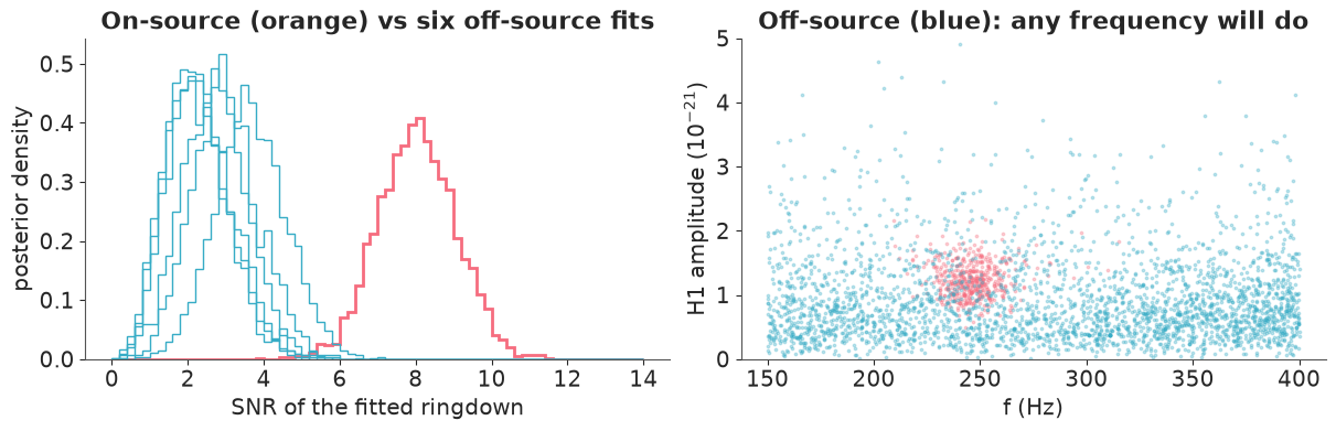
On noise, the frequency posterior simply returns its prior (an sd of 67-81 Hz, against
72 Hz for Uniform(150, 400)) and the fitted SNR has a median of 2-4 - not zero, because a
norm is positive and a flexible template can always soak up a little noise. On-source the
SNR posterior sits clearly apart and the draws form one tight cluster in the right panel.
Note what does not discriminate: the amplitude. Off-source medians are 0.5-1, not far
below the on-source 1.2, because a large amplitude with a very short damping time costs
almost nothing in SNR. The question "is the amplitude zero?" is the wrong one; "does the
template explain variance?" is the right one. Several off-source fits show divergences
(up to 11 here) and an r_hat up to 1.03: with no signal, the posterior is the awkward
union of "small template, any frequency" and a few weak noise bumps. That is a property
of the question, not a bug to tune away.
3.2 · A Bayes factor that actually computes
"Signal versus noise" is a comparison between our model and the same model with all four amplitudes set to zero, which has no free parameters at all. Bayes factors are notoriously hard to compute, but this problem has structure: given $(f, \tau)$, the whitened template is linear in the four quadratures, with Gaussian priors and Gaussian noise. The quadratures can be integrated out in closed form (it is Bayesian linear regression with design matrix $X = L^{-1}[e^{-t/\tau}\cos\omega t,\ e^{-t/\tau}\sin\omega t]$):
$$\log\frac{p(d \mid f,\tau)}{p(d \mid \text{noise})} = \tfrac12\, b^\top\!\big(G + s^{-2}I\big)^{-1} b - \tfrac12\log\det\!\big(I + s^2 G\big), \qquad G = X^\top X,\; b = X^\top L^{-1}d .$$
What is left is a two-dimensional integral over $(f, \tau)$, which a grid does to high accuracy in a few seconds (most of it spent whitening the basis once). No sampler, no tuning, no stochastic error.
f_grid = np.linspace(150, 400, 201)
tau_grid = np.geomspace(0.3, 50, 100)  # ms
tw = np.arange(N_RING) / FS_FIT

ff, tt = np.meshgrid(f_grid, tau_grid, indexing="ij")
decay = np.exp(-tw / (tt[..., None] / 1e3))
basis = np.stack([decay * np.cos(2 * np.pi * ff[..., None] * tw), decay * np.sin(2 * np.pi * ff[..., None] * tw)], axis=-1)
X_GRID = {det: np.einsum("ij,ftjk->ftik", W_RING[det], basis) for det in DETECTORS}  # whitened basis, every grid point
G_GRID = {det: np.einsum("ftik,ftil->ftkl", X_GRID[det], X_GRID[det]) for det in DETECTORS}

# prior mass of each grid cell: uniform in f, log-normal in tau
log_prior_grid = stats.lognorm(s=0.75, scale=4).logpdf(tau_grid) + np.log(np.gradient(tau_grid))
log_prior_grid = (log_prior_grid - logsumexp(log_prior_grid))[None, :] - np.log(len(f_grid))


def log_bf_surface(whitened, amp_sd=AMP_SD):
    """log p(d | f, tau) / p(d | noise) on the grid, amplitudes marginalised. `whitened`: {det: L^-1 d}."""
    out = 0.0
    for det in DETECTORS:
        b = np.einsum("ftik,i->ftk", X_GRID[det], whitened[det])
        A = G_GRID[det] + np.eye(2) / amp_sd**2
        out = out + 0.5 * np.einsum("ftk,ftk->ft", b, np.linalg.solve(A, b[..., None])[..., 0])
        out = out - 0.5 * np.log(np.linalg.det(np.eye(2) + amp_sd**2 * G_GRID[det]))
    return out


def log_bayes_factor(whitened, amp_sd=AMP_SD):
    return logsumexp(log_bf_surface(whitened, amp_sd) + log_prior_grid)


on_source = {det: ring_parts[det][2] for det in DETECTORS}
log_bf_on = log_bayes_factor(on_source)
print(f"on-source: ln BF (signal : noise) = {log_bf_on:.1f}   ->   BF ~ {np.exp(log_bf_on):.1e}")
on-source: ln BF (signal : noise) = 19.7 -> BF ~ 3.5e+08
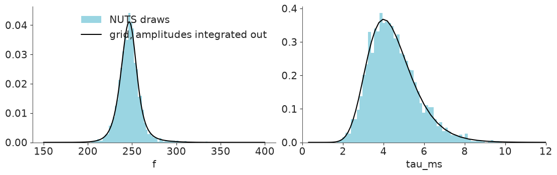
Cross-check 1: the grid reproduces NUTS. The same grid gives the exact marginal posterior of $(f, \tau)$, which should match the PyMC fit from 2.4.
log_post = log_bf_surface(on_source) + log_prior_grid
post_grid = np.exp(log_post - logsumexp(log_post))

fig, axes = plt.subplots(1, 2, figsize=(11, 3.4))
for ax, v, g, marginal in [(axes[0], "f", f_grid, post_grid.sum(axis=1)), (axes[1], "tau_ms", tau_grid, post_grid.sum(axis=0))]:
    ax.hist(ring_idata.posterior[v].values.ravel(), bins=60, density=True, alpha=0.5, label="NUTS draws")
    ax.plot(g, marginal / np.gradient(g), "k", label="grid, amplitudes integrated out")
    ax.set(xlabel=v)
axes[1].set_xlim(0, 12)
axes[0].legend(loc="upper right");
Cross-check 2: Sequential Monte Carlo. pm.sample_smc tempers from the prior to the
posterior and estimates the marginal likelihood as a by-product. It runs fine in PyMC 6;
the estimate lives in sample_stats["log_marginal_likelihood"] as an object array with one
entry per tempering stage, of which only the last is the final estimate. To turn it into a
Bayes factor, subtract the log-likelihood of the noise model, which is just the standard
normal log-density of the whitened data.
with ring_model:
    # SMC runs one worker PROCESS per core, each with its own copy of the model: cores=2 keeps memory in check
    smc_idata = pm.sample_smc(2000, chains=4, cores=2, random_seed=RANDOM_SEED, progressbar=False)

log_z_noise = sum(stats.norm.logpdf(on_source[det]).sum() for det in DETECTORS)
log_z_smc = np.array([
    np.asarray(chain, dtype=float)[np.isfinite(np.asarray(chain, dtype=float))][-1]
    for chain in smc_idata.sample_stats["log_marginal_likelihood"].values
])
print("ln BF from SMC, per chain:", (log_z_smc - log_z_noise).round(2), f"   grid: {log_bf_on:.2f}")
ln BF from SMC, per chain: [19.57 19.74 19.59 19.74] grid: 19.68
The four SMC chains agree with one another and with the grid to within about 0.2. Two independent methods, one number: $\ln \text{BF} \approx 19.7$, odds of a few hundred million to one. For a generic model you would have only SMC (or bridge sampling, or nested sampling); the lesson of the grid is to look for conditionally linear-Gaussian structure first, because integrating parameters out analytically beats any sampler.
But what is a Bayes factor of $10^8$ worth? It compares our two models: "Gaussian noise plus a damped sinusoid" versus "Gaussian noise". Real detectors glitch, and a glitch is neither. The empirical answer is to compute the same statistic where we know there is no astrophysical signal, and see what the noise can do: a background distribution. Because the grid is fast, we can afford every non-overlapping off-source window.
bg_times = np.arange(-13, 15, 0.11)
bg_times = bg_times[np.abs(bg_times) > 1]


def whitened_at(t_start, extra=None):
    out = {}
    for k, det in enumerate(DETECTORS):
        i = np.searchsorted(t_fit, t_start - (DT_HL if det == "L1" else 0.0))
        d = cond[det][i : i + N_RING] + (0 if extra is None else extra[k])
        out[det] = W_RING[det] @ d
    return out


log_bf_bg = np.array([log_bayes_factor(whitened_at(ts)) for ts in bg_times])
print(f"{len(bg_times)} off-source windows: ln BF from {log_bf_bg.min():.1f} to {log_bf_bg.max():.1f}, "
      f"{(log_bf_bg > 0).sum()} of them favour a signal")

amp_sds = np.array([0.25, 0.5, 1, 2, 5, 10, 30, 100])
log_bf_vs_prior = [log_bayes_factor(on_source, s) for s in amp_sds]

fig, axes = plt.subplots(1, 2, figsize=(12, 3.6))
axes[0].hist(log_bf_bg, bins=30, label="off-source windows")
axes[0].axvline(log_bf_on, color="C1", lw=2, label="on-source")
axes[0].set(xlabel="ln Bayes factor (signal : noise)", ylabel="windows", title="Background distribution")
axes[0].legend()
axes[1].semilogx(amp_sds, log_bf_vs_prior, "o-")
axes[1].axvline(AMP_SD, color="k", ls=":", label="prior used")
axes[1].set(xlabel="prior sd of the amplitude quadratures ($10^{-21}$)", ylabel="on-source ln BF",
            title="Sensitivity to the amplitude prior")
axes[1].legend();
237 off-source windows: ln BF from -6.9 to -0.7, 0 of them favour a signal
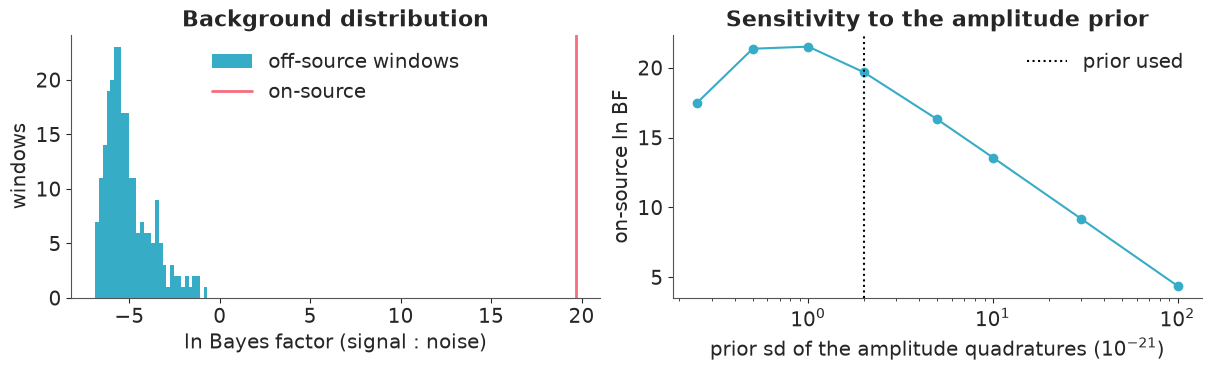
Every one of the off-source windows has a negative log Bayes factor: when there is nothing there, the evidence (mildly) prefers the simpler model - Occam's razor working as advertised. The on-source value is far outside anything the noise produced. With a couple of hundred windows that supports a false-alarm probability below about 1 in 200 for this statistic and no more; LIGO's "less than one in 200,000 years" comes from time-sliding weeks of data from the two sites against each other, which 32 seconds cannot imitate.
The right panel is the standard health warning. The Bayes factor depends on the prior width: make the amplitude prior absurdly wide and the signal model is penalised for all the loud signals it predicted and did not see (roughly $-4\ln s$ for four amplitudes). Here the conclusion survives any remotely sensible choice, but the number is only meaningful together with the prior that produced it.
3.3 · Is the likelihood calibrated on real noise? (SBC, for free)
The exact grid posterior makes simulation-based calibration cheap: draw parameters from the prior, add the corresponding ringdown to a real off-source noise window, compute the posterior, and record where the truth falls in it. If the whole pipeline - noise model, whitening, priors - is right, those posterior CDF values are uniform. Unlike a test on simulated Gaussian noise, this one can fail if the real noise is not what our likelihood assumes.
sbc_rng = np.random.default_rng(RANDOM_SEED)
pit = {"f": [], "tau_ms": []}
for ts in bg_times:
    f_true = sbc_rng.uniform(150, 400)
    tau_true = np.exp(sbc_rng.normal(np.log(4), 0.75))
    quad = sbc_rng.normal(0, AMP_SD, size=(2, 2))
    injected = [ringdown_np(tw, f_true, tau_true, *quad[k]) for k in range(2)]
    lp = log_bf_surface(whitened_at(ts, extra=injected)) + log_prior_grid
    pg = np.exp(lp - logsumexp(lp))
    marg_f, marg_tau = pg.sum(axis=1), pg.sum(axis=0)
    # posterior CDF at the truth, interpolated between grid points
    pit["f"].append(np.interp(f_true, f_grid, np.cumsum(marg_f) - 0.5 * marg_f))
    pit["tau_ms"].append(np.interp(np.log(tau_true), np.log(tau_grid), np.cumsum(marg_tau) - 0.5 * marg_tau))

fig, axes = plt.subplots(1, 2, figsize=(10, 3.2), sharey=True)
for ax, (v, values) in zip(axes, pit.items()):
    values = np.array(values)
    ax.hist(values, bins=10, range=(0, 1))
    ax.axhline(len(values) / 10, color="k", ls="--")
    ax.set(xlabel=f"posterior CDF at the true {v}")
    print(f"{v:<7} KS test against uniform: p = {stats.kstest(values, 'uniform').pvalue:.2f}   "
          f"coverage of the central 90% interval: {np.mean((values > 0.05) & (values < 0.95)):.2f}")
axes[0].set_ylabel("simulations");
f       KS test against uniform: p = 0.52   coverage of the central 90% interval: 0.92
tau_ms  KS test against uniform: p = 0.91   coverage of the central 90% interval: 0.89
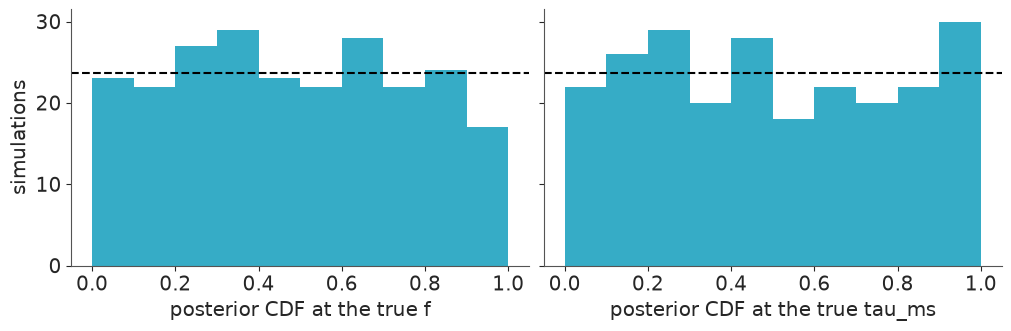
Histograms compatible with flat, and 90% intervals that cover the truth 92% and 89% of the time, with 237 simulations (so a binomial standard error of 2 points) on real detector noise. Do not read more into it than that: for the loudest prior draws the posterior is narrower than a grid cell, which limits this check to a few points of coverage (repeating it with other seeds gives 88-94%). Within that resolution the machinery - noise covariance, whitening, marginalisation, priors - is calibrated. It says nothing about whether a single damped sinusoid is the right model for what GW150914 did 3 ms after its peak - that was section 2.6.
3.4 · How detection is actually done: the matched filter
LIGO's search pipelines do not run MCMC on every second of data. They slide templates across the data and compute, for every arrival time at once (one FFT),
$$\rho(t) = \frac{|\langle d, h_t\rangle|}{\sqrt{\langle h, h\rangle}}, \qquad \langle a, b\rangle = 4\,\mathrm{Re}\!\int_0^\infty \frac{\tilde a(f)\,\tilde b^*(f)}{S(f)}\,df .$$
That inner product is the Whittle likelihood again: for fixed template shape, $\rho^2/2$ is the log-likelihood ratio maximised over amplitude, and taking the modulus of the complex filter output maximises over phase. The matched filter is the maximum-likelihood cousin of the marginalisation we just did - the same two quadratures, maximised instead of integrated. In Gaussian noise $\rho$ of a few is typical and 5 is already rare.
We use two templates: our ringdown (posterior medians from 2.4), and the inspiral chirp of Part 4 at leading order, for a small bank of chirp masses.
def matched_filter(x, template, psd_grid, f_lo=30.0, f_hi=500.0):
    """|SNR| time series; `template` is sampled like `x`, with its reference time at index 0 (wrapping around)."""
    df = freqs[1]
    band = (freqs >= f_lo) & (freqs <= f_hi)
    x_f = np.fft.rfft(x * taper) * dt
    h_f = np.fft.rfft(template) * dt
    integrand = np.zeros(n_samples, dtype=complex)  # positive frequencies only -> complex SNR (both phases)
    integrand[: len(freqs)] = np.where(band, x_f * np.conj(h_f) / psd_grid, 0)
    z = 4 * np.fft.ifft(integrand) * n_samples * df
    sigma_sq = 4 * np.sum(np.where(band, np.abs(h_f) ** 2 / psd_grid, 0)) * df
    return np.abs(z) / np.sqrt(sigma_sq)


def newtonian_chirp_template(chirp_mass, f_min=25.0, stop=0.004):
    """Leading-order inspiral ending at index 0 (i.e. the SNR is reported at the coalescence time)."""
    to_merger = (n_samples - np.arange(n_samples)) * dt
    m_sec = chirp_mass * MSUN_S
    f_gw = (5 / (256 * to_merger)) ** 0.375 * m_sec**-0.625 / np.pi
    phase = -2 * (to_merger / (5 * m_sec)) ** 0.625
    return np.where((f_gw > f_min) & (to_merger > stop), to_merger**-0.25 * np.cos(phase), 0.0)


t_since_start = np.arange(n_samples) * dt
f_med, tau_med = float(ring_idata.posterior["f"].median()), float(ring_idata.posterior["tau_ms"].median())
ring_template = np.exp(-t_since_start / (tau_med / 1e3)) * np.cos(2 * np.pi * f_med * t_since_start)

inner = (t > t[0] + 2) & (t < t[-1] - 2)  # stay away from the tapered edges
bank = np.arange(20, 52, 2)
bank_snr = {det: np.array([matched_filter(strain[det], newtonian_chirp_template(mc), psd_on_grid[det])[inner].max() for mc in bank])
            for det in DETECTORS}
best_mc = bank[np.argmax(np.sqrt(bank_snr["H1"] ** 2 + bank_snr["L1"] ** 2))]

fig, axes = plt.subplots(1, 3, figsize=(14, 3.6))
for det in DETECTORS:
    snr_chirp = matched_filter(strain[det], newtonian_chirp_template(best_mc), psd_on_grid[det])
    snr_ring = matched_filter(strain[det], ring_template, psd_on_grid[det])
    far = inner & (np.abs(t - T_PEAK) > 0.5)
    print(f"{det}: chirp template peak SNR {snr_chirp[inner].max():.1f} at t = {1e3 * t[inner][snr_chirp[inner].argmax()]:.1f} ms "
          f"(loudest elsewhere {snr_chirp[far].max():.1f});   ringdown template peak SNR {snr_ring[inner].max():.1f} "
          f"at t = {1e3 * t[inner][snr_ring[inner].argmax()]:.1f} ms (elsewhere {snr_ring[far].max():.1f})")
    if det == "H1":
        axes[0].plot(t[inner], snr_chirp[inner], lw=0.6, label=f"chirp template, {best_mc} $M_\\odot$")
        axes[0].plot(t[inner], snr_ring[inner], lw=0.6, label="ringdown template")
    axes[1].plot(t[inner] * 1e3, snr_chirp[inner], label=det)
    axes[2].plot(bank, bank_snr[det], "o-", label=det)
axes[0].set(xlabel="time from event (s)", ylabel="matched-filter SNR", title="H1: 28 s of SNR time series")
axes[0].legend(loc="upper left")
axes[1].set(xlim=(-30, 70), xlabel="time from event (ms)", title="Zoom: chirp template, both detectors")
axes[1].legend()
axes[2].set(xlabel=r"template chirp mass ($M_\odot$)", ylabel="peak SNR", title="A tiny template bank")
axes[2].legend()
print(f"network SNR of the best chirp template: {np.sqrt(bank_snr['H1'].max() ** 2 + bank_snr['L1'].max() ** 2):.1f}")
H1: chirp template peak SNR 17.0 at t = 26.5 ms (loudest elsewhere 4.3);   ringdown template peak SNR 9.2 at t = 25.0 ms (elsewhere 4.4)
L1: chirp template peak SNR 11.0 at t = 18.9 ms (loudest elsewhere 4.8);   ringdown template peak SNR 8.3 at t = 17.5 ms (elsewhere 4.6)
network SNR of the best chirp template: 20.2
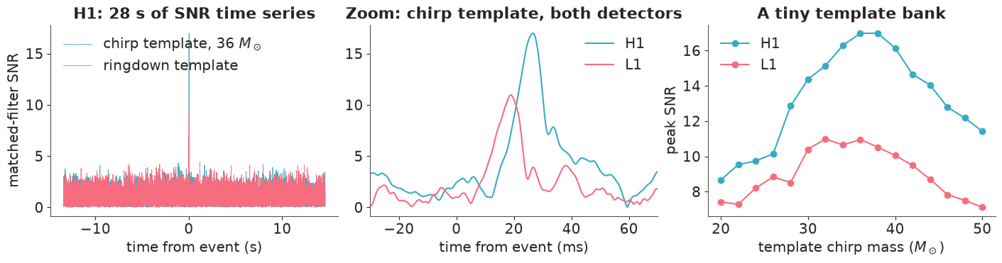
One spike in 28 seconds, in both detectors, at times 7-8 ms apart - against a background that never exceeds 5. The ringdown template alone reaches an SNR of 8-9 (it also rings on the merger, so this is higher than the SNR of the post-$t_0$ fit in Part 2); the chirp template collects the whole inspiral and does far better. Our network SNR of about 20 falls short of the published 24 because a leading-order inspiral that stops 4 ms before merger is a cruder template than the ones LIGO uses.
Note where the little template bank peaks: at a chirp mass of 36-38 $M_\odot$, not the published value of about 30. Hold that thought.
Part 4 (stretch) · The inspiral chirp
Before they merge, two masses in orbit lose energy to gravitational waves, so the orbit shrinks and speeds up. At leading ("Newtonian quadrupole") order the gravitational-wave frequency and phase depend on the masses only through the chirp mass $\mathcal{M} = (m_1 m_2)^{3/5}/(m_1+m_2)^{1/5}$:
$$f(t) = \frac{1}{\pi}\left(\frac{5}{256\,(t_c - t)}\right)^{3/8}\left(\frac{G\mathcal{M}}{c^3}\right)^{-5/8}, \qquad \Phi(t) = -2\left(\frac{t_c - t}{5\,G\mathcal{M}/c^3}\right)^{5/8}, \qquad h(t) \propto f^{2/3}\cos(\Phi(t) + \varphi_c) \propto (t_c-t)^{-1/4}\cos(\dots)$$
where $t_c$ is the (formal) coalescence time at which the frequency diverges. We fit the 185 ms that end 15 ms before the peak - where the approximation is least bad - with exactly the machinery of Part 2: a 379-sample window per detector, the full noise covariance, L1 aligned by the Part 1 shift. Priors: $\mathcal{M} \sim \text{Uniform}(15, 60)\,M_\odot$ and $t_c \sim \mathcal{N}(t_\text{peak}, 5\text{ ms})$, because the frequency visibly stops rising at the peak.
4.1 · The obvious parameterisation, and how it fails
Amplitude and phase at coalescence per detector - what you would write down first.
T_CHIRP = (T_PEAK - 0.200, T_PEAK - 0.015)

chirp_parts = {}
for det in DETECTORS:
    shift = DT_HL if det == "L1" else 0.0
    i0, i1 = np.searchsorted(t_fit, [T_CHIRP[0] - shift, T_CHIRP[1] - shift])
    W = whitener(det, i1 - i0)
    chirp_parts[det] = (t_fit[i0:i1] + shift, W, W @ cond[det][i0:i1])  # times on the H1 clock
print({det: len(v[0]) for det, v in chirp_parts.items()}, "samples per detector")


def chirp_phase_amp(chirp_mass, tc, times, xp=pt):
    to_merger = xp.maximum(tc - times, 1e-4)
    return -2 * (to_merger / (5 * chirp_mass * MSUN_S)) ** 0.625, (to_merger / 0.1) ** -0.25


with pm.Model(coords={"det": DETECTORS}) as chirp_naive:
    chirp_mass = pm.Uniform("chirp_mass", 15, 60)
    tc_ms = pm.Normal("tc_ms", 0, 5)  # coalescence time relative to T_PEAK, in ms
    A = pm.HalfNormal("A", AMP_SD, dims="det")  # amplitude 0.1 s before coalescence
    phi_c = pm.Uniform("phi_c", -np.pi, np.pi, dims="det")
    for k, det in enumerate(DETECTORS):
        times, W, y = chirp_parts[det]
        phase, growth = chirp_phase_amp(chirp_mass, T_PEAK + tc_ms / 1e3, times)
        pm.Normal(f"y_{det}", mu=pt.dot(W, A[k] * growth * pt.cos(phase + phi_c[k])), sigma=1, observed=y)
    naive_idata = pm.sample(random_seed=RANDOM_SEED)

print("divergences:", int(naive_idata.sample_stats["diverging"].sum()))
az.summary(naive_idata, round_to=2)
{'H1': 379, 'L1': 379} samples per detectordivergences: 0
| mean | sd | eti89_lb | eti89_ub | ess_bulk | ess_tail | r_hat | mcse_mean | mcse_sd | |
|---|---|---|---|---|---|---|---|---|---|
| tc_ms | 4.30 | 4.55 | -2.07 | 11.62 | 5.41 | 10.93 | 2.07 | 2.11 | 0.75 |
| chirp_mass | 37.19 | 1.93 | 34.14 | 40.08 | 5.62 | 11.60 | 1.95 | 0.85 | 0.27 |
| A[H1] | 0.56 | 0.07 | 0.46 | 0.68 | 34.19 | 70.02 | 1.09 | 0.01 | 0.00 |
| A[L1] | 0.36 | 0.07 | 0.26 | 0.47 | 1566.87 | 2200.81 | 1.01 | 0.00 | 0.00 |
| phi_c[H1] | 0.47 | 1.74 | -2.76 | 2.85 | 5.91 | 11.49 | 1.84 | 0.78 | 0.34 |
| phi_c[L1] | -0.88 | 1.57 | -2.99 | 1.94 | 5.77 | 11.24 | 1.89 | 0.68 | 0.28 |
fig, axes = plt.subplots(1, 2, figsize=(11, 3.8))
for c in naive_idata.posterior.chain.values:
    pc = naive_idata.posterior.sel(chain=c)
    axes[0].scatter(pc["tc_ms"], pc["phi_c"].sel(det="H1"), s=3, alpha=0.4, label=f"chain {c}")
    axes[1].scatter(pc["tc_ms"], pc["chirp_mass"], s=3, alpha=0.4)
axes[0].set(xlabel="$t_c - t_{peak}$ (ms)", ylabel=r"$\varphi_c$ (H1)", ylim=(-np.pi, np.pi), title="Each chain owns a piece of the ridge")
axes[0].legend(markerscale=4, loc="lower right")
axes[1].set(xlabel="$t_c - t_{peak}$ (ms)", ylabel=r"chirp mass ($M_\odot$)");
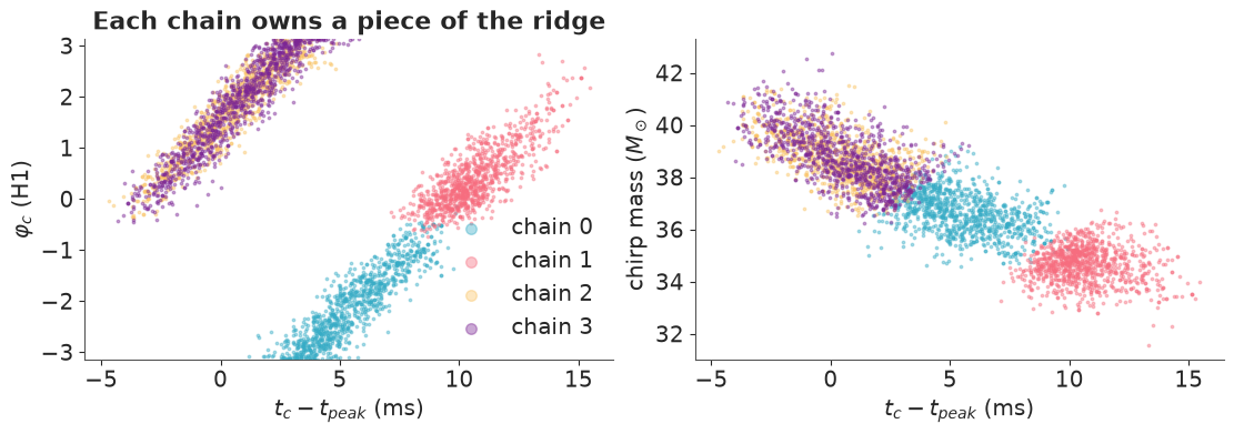
An r_hat of about 2 and an ESS in single digits for $t_c$ and the chirp mass: the chains
disagree, and no divergence warned us. The left panel shows why. The phase at
coalescence is an extrapolation of the phase in the window, so it is almost perfectly
correlated with $t_c$: moving $t_c$ by several milliseconds winds $\varphi_c$ through a
full turn. The posterior is one long diagonal ridge wrapped around a cylinder - where it
leaves the plot at $+\pi$ it re-enters at $-\pi$ - but to NUTS the $\pm\pi$ edges of the
Uniform prior are walls. With two detectors, each with its own wrapped phase, the ridge
is chopped into several pieces; each chain explores the piece it started in, and so sees
only part of the $t_c$-$\mathcal{M}$ range (right panel). This is the $(t_c, \varphi)$
multimodality every gravitational-wave sampler has to deal with; more tuning or a higher
target_accept will not fix it.
4.2 · The fix: integrate the nuisance parameters out
The trouble lives entirely in amplitude and phase, which we do not care about - and, as
in 3.2, in quadrature form the template is linear in them. So marginalise them
analytically. What remains is a two-parameter posterior for $(\mathcal{M}, t_c)$, which
we can both map exactly on a grid and hand to NUTS via pm.Potential. (Production codes
do the same thing: phase, and often time and distance, are marginalised analytically
before the sampler sees the problem.)
def chirp_basis(chirp_mass, tc, times, pn_order=0, eta=0.25):
    """Whitened-ready quadrature basis. pn_order > 0 adds post-Newtonian phase corrections (section 4.3)."""
    to_merger = np.maximum(tc - times, 1e-4)
    total_mass = chirp_mass * MSUN_S / eta**0.6
    theta = eta * to_merger / (5 * total_mass)
    series = theta**0.625
    if pn_order >= 1:
        series = series + (3715 / 8064 + 55 / 96 * eta) * theta**0.375
    if pn_order >= 1.5:
        series = series - 0.75 * np.pi * theta**0.25
    phase = -2 / eta * series
    growth = (to_merger / 0.1) ** -0.25
    return np.stack([growth * np.cos(phase), growth * np.sin(phase)], axis=1)


def chirp_log_bf_grid(mc_grid, tc_grid_ms, pn_order=0):
    out = np.zeros((len(mc_grid), len(tc_grid_ms)))
    for i, mc in enumerate(mc_grid):
        for j, tc in enumerate(tc_grid_ms):
            for det in DETECTORS:
                times, W, y = chirp_parts[det]
                X = W @ chirp_basis(mc, T_PEAK + tc / 1e3, times, pn_order)
                G, b = X.T @ X, X.T @ y
                out[i, j] += 0.5 * b @ np.linalg.solve(G + np.eye(2) / AMP_SD**2, b)
                out[i, j] -= 0.5 * np.log(np.linalg.det(np.eye(2) + AMP_SD**2 * G))
    return out


mc_grid = np.linspace(15, 60, 91)
tc_grid = np.linspace(-14, 25, 79)
chirp_surface = chirp_log_bf_grid(mc_grid, tc_grid)
print(f"maximum ln BF on the grid: {chirp_surface.max():.1f}")
maximum ln BF on the grid: 47.9
with pm.Model() as chirp_marginal:
    chirp_mass = pm.Uniform("chirp_mass", 15, 60)
    tc_ms = pm.Normal("tc_ms", 0, 5)
    log_like = 0
    for det in DETECTORS:
        times, W, y = chirp_parts[det]
        phase, growth = chirp_phase_amp(chirp_mass, T_PEAK + tc_ms / 1e3, times)
        x_c, x_s = pt.dot(W, growth * pt.cos(phase)), pt.dot(W, growth * pt.sin(phase))
        # 2 x 2 linear algebra written out: A = X'X + I/s^2, b = X'y
        a11, a22, a12 = pt.sum(x_c**2) + AMP_SD**-2, pt.sum(x_s**2) + AMP_SD**-2, pt.sum(x_c * x_s)
        b1, b2 = pt.sum(x_c * y), pt.sum(x_s * y)
        det_a = a11 * a22 - a12**2
        log_like += 0.5 * (a22 * b1**2 - 2 * a12 * b1 * b2 + a11 * b2**2) / det_a - 0.5 * pt.log(det_a * AMP_SD**4)
    pm.Potential("marginal_loglike", log_like)
    # start where the matched filter of 3.4 pointed, as real pipelines do
    chirp_idata = pm.sample(random_seed=RANDOM_SEED, initvals={"chirp_mass": float(best_mc), "tc_ms": 0.0})

print("divergences:", int(chirp_idata.sample_stats["diverging"].sum()))
az.summary(chirp_idata, ci_kind="eti", ci_prob=0.9, round_to=2)
divergences: 0
| mean | sd | eti90_lb | eti90_ub | ess_bulk | ess_tail | r_hat | mcse_mean | mcse_sd | |
|---|---|---|---|---|---|---|---|---|---|
| tc_ms | 2.81 | 3.65 | -2.86 | 8.88 | 859.86 | 861.88 | 1.0 | 0.12 | 0.10 |
| chirp_mass | 37.82 | 1.65 | 35.15 | 40.61 | 832.51 | 834.34 | 1.0 | 0.06 | 0.04 |
log_prior_chirp = stats.norm(0, 5).logpdf(tc_grid)[None, :]
chirp_post = np.exp(chirp_surface + log_prior_chirp - (chirp_surface + log_prior_chirp).max())
cd = az.extract(chirp_idata, num_samples=1500, random_seed=RANDOM_SEED)

fig, axes = plt.subplots(1, 2, figsize=(12, 4))
mesh = axes[0].pcolormesh(tc_grid, mc_grid, chirp_surface, vmin=-5, shading="auto", cmap="viridis")
axes[0].grid(False)
fig.colorbar(mesh, ax=axes[0], label="ln BF")
axes[0].set(xlabel="$t_c - t_{peak}$ (ms)", ylabel=r"chirp mass ($M_\odot$)", title="Nuisance parameters integrated out")
axes[1].contour(tc_grid, mc_grid, chirp_post, levels=[0.01, 0.1, 0.5, 0.9], colors="k", linewidths=1)
axes[1].scatter(cd["tc_ms"], cd["chirp_mass"], s=3, alpha=0.3, color="C1")
axes[1].set(xlabel="$t_c - t_{peak}$ (ms)", ylabel=r"chirp mass ($M_\odot$)", ylim=(28, 48),
            title="Posterior: grid contours, NUTS draws");
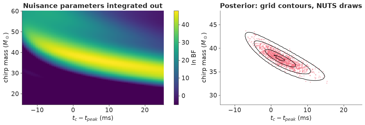
With the nuisance parameters gone the broken ridge is gone: the marginal likelihood is a
single smooth, curved ridge (a later coalescence time trades against a lower chirp mass),
NUTS samples it without complaint, and the draws sit on the exact grid contours. One more
honest detail: below the ridge the surface is a flat plateau with no gradient, and a chain
initialised there can sit on it for the whole run. That is why we passed initvals from
the matched-filter peak - which is precisely how real parameter estimation is seeded by
the search pipelines.
4.3 · The error the posterior cannot see
So: a chirp mass of about $38 \pm 2\,M_\odot$, tidy diagnostics, agreement between grid, NUTS and the matched-filter bank. The published detector-frame value is about 30-31 $M_\odot$. We are off by four of our own standard deviations.
The posterior is a statement about the parameters given the model, and the model is the leading term of an expansion in $v/c$ - applied to two roughly 30 $M_\odot$ black holes in their last few orbits, moving at a third to a half of the speed of light. The next terms of the post-Newtonian series (for the phase, in the "TaylorT3" form, with $\Theta = \eta (t_c-t)/(5GM/c^3)$, total mass $M$ and symmetric mass ratio $\eta$) are
$$\Phi = -\frac{2}{\eta}\left[\Theta^{5/8} + \left(\tfrac{3715}{8064} + \tfrac{55}{96}\eta\right)\Theta^{3/8} - \tfrac{3\pi}{4}\,\Theta^{1/4} + \dots\right].$$
Fixing equal masses ($\eta = 1/4$) keeps the parameter count unchanged, and the grid makes the experiment cheap:
rows = []
mc_wide = np.linspace(20, 60, 81)
for order, label in [(0, "Newtonian (0PN)"), (1, "+ 1PN"), (1.5, "+ 1PN + 1.5PN")]:
    surf = chirp_surface if order == 0 else chirp_log_bf_grid(mc_wide, tc_grid, order)
    grid_mc = mc_grid if order == 0 else mc_wide
    weights = np.exp(surf + log_prior_chirp - (surf + log_prior_chirp).max()).sum(axis=1)
    weights /= weights.sum()
    mean = np.sum(grid_mc * weights)
    rows.append({"phase model": label, "chirp mass mean": mean,
                 "sd": np.sqrt(np.sum((grid_mc - mean) ** 2 * weights)), "best ln BF": surf.max()})
pd.DataFrame(rows).set_index("phase model").round(1)
| chirp mass mean | sd | best ln BF | |
|---|---|---|---|
| phase model | |||
| Newtonian (0PN) | 37.8 | 1.7 | 47.9 |
| + 1PN | 51.6 | 2.5 | 48.0 |
| + 1PN + 1.5PN | 27.1 | 1.1 | 45.9 |
Three truncations of the same series fit the data equally well (the best log Bayes
factors are within about two units) and give chirp masses of roughly 38, 52 and 27
$M_\odot$, each with a confident-looking error bar of 1-3. The series is alternating and
converges slowly this close to merger; the published value lies between the rungs. The
statistical uncertainty is the small part of the error budget here, and
nothing in any single fit - not r_hat, not the residuals, not the Bayes factor - can
tell you so. Only varying the model can. This is why the LIGO-Virgo analyses use waveform
families calibrated against numerical solutions of Einstein's equations, run at least two
independent families, and report the difference as a systematic.
It is the same lesson as the golf putts in C01, at a rather different distance scale: a narrow posterior is not evidence that the model is right.
What to take away
- Coloured noise is handled by whitening - but whiten the template with the same operator, do not re-scale band-passed noise and pretend the samples are independent, and prefer the exact time-domain covariance when the model has a sharp edge in time.
- Reparameterise before you tune: quadratures instead of amplitude-phase; physical parameters (mass, spin) when the prior belief is physical.
- Linear-Gaussian sub-structure is gold: integrate it out. It gave us an exact posterior to check NUTS against, a Bayes factor without a sampler, a background distribution, SBC in seconds, and the cure for a multimodal sampler.
- Validate on noise and on injections drawn from the prior into real noise.
- Vary what you assumed - the start time, the prior, the waveform order. The largest uncertainties in this notebook were never inside a single posterior.
Try it yourself
- Add an overtone. Give the ringdown a second damped sinusoid (the $n = 1$ overtone)
with its own quadratures, start at $t_0 = t_\text{peak}$, and use
kerr_prior=True-style parameters so both modes share one mass and spin. Berti-Cardoso-Will coefficients for the 221 mode: $f_{1,2,3} = (1.3673, -1.0260, 0.1628)$ and $q_{1,2,3} = (0.1000, 0.5436, -0.4731)$ (check them against the paper's tables before you trust them - at $\chi = 0.69$ they should give a damping time of about 1.4 ms). Does the bias at $t_0 = t_\text{peak}$ in section 2.6 go away? How does the grid evidence change (you now have eight linear parameters per $(M, \chi)$ point)? - Do it in the frequency domain. Implement the Whittle likelihood for the chirp of
Part 4 (whose window has no sharp physical edge if you taper it): FFT the tapered
template with
pytensor.tensor.fft.rfftor a JAX function brought in withpytensor.wrap_jax, and compare the posterior with the time-domain one. Where do they differ, and why? - Let the chirp measure the time shift. Unlike a damped sinusoid, a chirp changes frequency, so a time shift is not a phase shift. Add the H1-L1 delay as a parameter of the marginalised chirp model (shift the L1 time axis inside the model) with a Uniform(-10, 10) ms prior. Is the posterior unimodal? How does it compare with 6.9 ms?
And when you are done: register the strain files of another event from gwosc.org in
data.py and point the notebook at them. GW190521 is almost all ringdown, GW170817 is
almost all inspiral - see which of the conclusions above survive.
Data credit and references
This research has made use of data obtained from the Gravitational Wave Open Science Center (gwosc.org), a service of the LIGO Scientific Collaboration, the Virgo Collaboration and KAGRA. See R. Abbott et al., "Open data from the first and second observing runs of Advanced LIGO and Advanced Virgo", SoftwareX 13 (2021) 100658.
- B. P. Abbott et al., "Observation of gravitational waves from a binary black hole merger", Phys. Rev. Lett. 116, 061102 (2016) - the detection, and the published values quoted above (with later updates in the GWTC-1 catalogue).
- B. P. Abbott et al., "Tests of general relativity with GW150914", Phys. Rev. Lett. 116, 221101 (2016) - the damped-sinusoid fit against start time.
- E. Berti, V. Cardoso and C. M. Will, Phys. Rev. D 73, 064030 (2006) - the quasi-normal mode fitting formulas.
- M. Isi and W. M. Farr, "Analyzing black-hole ringdowns", arXiv:2107.05609 - the time-domain likelihood used in Part 2; M. Isi et al., Phys. Rev. Lett. 123, 111102 (2019) for overtones.