import os

for v_ in ("OMP_NUM_THREADS", "OPENBLAS_NUM_THREADS", "MKL_NUM_THREADS"):
    os.environ[v_] = "1"  # nutpie runs chains as threads: one BLAS pool per chain would fight

import logging
import sys
import textwrap
import time
import warnings

import arviz as az
import matplotlib.pyplot as plt
import numpy as np
import nutpie
import pandas as pd
import pymc as pm
import pytensor
import pytensor.tensor as pt
from IPython.display import Markdown, display
from matplotlib.colors import to_rgb
from matplotlib.patches import Ellipse, Polygon, Rectangle

from pymc_challenges import data
from pymc_challenges import public as pub

RANDOM_SEED = 114
rng = np.random.default_rng(RANDOM_SEED)
az.style.use("arviz-variat")
logging.getLogger("pymc").setLevel(logging.WARNING)
warnings.filterwarnings("ignore", category=FutureWarning)
warnings.filterwarnings("ignore", category=RuntimeWarning)
warnings.filterwarnings("ignore", category=UserWarning)
sys.modules.pop("jax", None)  # arviz leaves a lazy jax stub that makes matplotlib import all of JAX
pd.set_option("display.width", 160)
T_START = time.time()
TIMES = {}
INK, MUTED, LIGHT, HI, LO = pub.INK, pub.MUTED, pub.LIGHT, pub.HI, pub.LO


def wrap(text, width=90):
    return "\n".join(textwrap.fill(t, width) for t in text.split("\n"))


print(f"PyMC {pm.__version__}, ArviZ {az.__version__}, nutpie {nutpie.__version__}")
PyMC 6.3.2, ArviZ 1.3.0, nutpie 0.16.11
In plain words
The question. When I buy cod, sole or hake, is the population in the sea healthy, or has it been fished down?
What we did. For 18 fish stocks from North America, Chile, Australia and New Zealand we rebuilt the hidden amount of fish in the sea each year from catches and surveys. Each stock is a savings account: it earns the most interest at half its natural size, and catches are withdrawals. How fast each kind of fish grows is built in from biology.
What we found. In the last year of each stock's data (2001-2015, not today), about 6 of the 18 (roughly 3 to 9) were below the healthy level, the size that gives the largest catch that can be taken year after year. Only one was more likely than not fished too hard. Catches alone missed the northern cod collapse.
HOW_SURE = display(Markdown("**How sure are we.** *Filled in from the fits in part E.*"),
                   display_id=True)
HEADLINE = display(Markdown("*The headline figure is drawn in part G from the fits below and "
                            "appears here once the notebook has run.*"), display_id=True)
How sure are we. It is very likely (94%) that at least 4 of the 18 were below the healthy level then. We have low confidence in that figure: the model is simpler than the official assessments and, where they disagree, usually the more optimistic, so if anything it undercounts.
The setting
On 2 July 1992 Canada closed the northern cod fishery off Newfoundland. A stock that had supported fishers for five centuries had fallen, in the official reconstruction, to about a twentieth of the level that gives the largest sustainable catch, and some 30,000 people lost their work. Hutchings & Myers (1994, Can. J. Fish. Aquat. Sci.) asked how the scientists had missed it: catch rates in the commercial fishery held up while the fish shrank, because boats kept finding the last dense schools. What is caught is not what is in the sea, and the gap between them has to be modelled, with its uncertainty stated.
The oldest model for that gap is a surplus-production model (Schaefer 1954; Pella & Tomlinson 1969). A stock of biomass $B$ grows logistically towards a carrying capacity $K$ at intrinsic rate $r$, and the catch $C$ is taken out:
$$B_{t+1} = B_t + r B_t \left(1 - \frac{B_t}{K}\right) - C_t .$$
The growth term is the "interest" of a savings account. It is largest when the stock is at half its unfished size, $B_{MSY} = K/2$, where it equals the maximum sustainable yield $MSY = rK/4$; a fishing mortality above $F_{MSY} = r/2$ drains the account. The ratios $B/B_{MSY}$ and $F/F_{MSY}$ are the coordinates of the Kobe plot that tuna commissions and many national agencies use to report stock status.
We never see $B$. We see the catch, and an index (a research survey, or the catch per hour of the fleet) assumed proportional to $B$ with noise. Meyer & Millar (1999, Can. J. Fish. Aquat. Sci.) wrote this as a Bayesian state-space model: each year's biomass is a latent state with process error (good and bad years for the fish), and the index observes it with observation error. Punt & Hilborn (1997, Reviews in Fish Biology and Fisheries) made the case for Bayesian assessment; JABBA (Winker, Carvalho & Kapur 2018, Fisheries Research) is a modern version. The prior on $r$ is where biology enters: CMSY (Froese et al. 2017, Fish and Fisheries) turns FishBase's resilience category into a range for $r$, and we start from the same ranges.
The data come from the RAM Legacy Stock Assessment Database (Ricard, Minto, Jensen & Baum 2012, Fish and Fisheries), which collects the inputs and outputs of formal assessments around the world, so for 14 of our stocks there is an official answer to compare with. Those are usually age-structured models with far more data: agreement is a check, not proof, and disagreement is a question, not a verdict on either.
| part | question | tool |
|---|---|---|
| A | What do catches and an index look like? | Pacific cod, Hecate Strait; the surplus curve |
| B | What can a stock's history tell us? | a toy stock, one-way and two-way trips |
| C | How does one real stock fit? | centred free states, a prior check, two failures |
| D | What do 18 stocks share? | family priors for r, one process noise, official assessments |
| E | Below the healthy level, and still fished hard? | Kobe probabilities, one decisive noise |
| F | What if we only had the catches? | northern cod, catch-only refits |
| G | How do we explain it to everyone? | 40 possible histories, fish icons, an MSY band, a GIF |
A · Catches, an index and a savings account
The data
tools/build_e114_ram.py downloads the RAM v4.44 archive, reads its R tables once with Rscript,
and keeps one row per stock and year from the first to the last catch year. We kept stocks with
at least 25 years of catch and at least 15 years of an index, and the script checks each index
against the assessment's own biomass, where RAM has one, to catch copies: the Peruvian anchoveta's
"survey" equals its assessed biomass in every year, so it is not an independent index and the
anchoveta stays in the file only as a catch-only row. Each stock carries its FishBase resilience
and the matching range for $r$. Beyond the copy test the choice was a judgement made while
looking at the data: three more candidates (Greenland halibut, Gulf of St Lawrence cod, St Pierre
pollock) were left out after we saw how their index compared with the assessed biomass
(correlations 0.03 and 0.54, and one with nothing to compare), while Hecate Strait rock sole was
kept although its catch rate runs against the assessed biomass (correlation -0.17; its short
survey agrees better, 0.40).
data.describe("e114_ram_stocks")
RAM = data.load("e114_ram_stocks")
NICE = {
    "PCODHS": "Pacific cod, Hecate Strait", "PCODWCVANI": "Pacific cod, W. Vancouver Island",
    "PCOD5AB": "Pacific cod, Queen Charlotte Sound", "RSOLEHSTR": "Rock sole, Hecate Strait",
    "RSOLE5AB": "Rock sole, Queen Charlotte Sound", "YELL3LNO": "Yellowtail flounder, Grand Banks",
    "YELLGB": "Yellowtail flounder, Georges Bank",
    "WITFLOUN4RST": "Witch flounder, Gulf of St Lawrence",
    "SPHAKECH": "Hake, Chile", "SHAKE4VWX": "Silver hake, Scotian Shelf",
    "SHAKESGBMATL": "Silver hake, S. Georges Bank-Mid-Atlantic",
    "SHAKEGOMNGB": "Silver hake, Gulf of Maine", "REDFISHSPP3LN": "Redfish, Grand Banks",
    "NZSNAPNZ7": "Snapper, New Zealand (SNA 7)", "TREVALLYTRE7": "Trevally, New Zealand (TRE 7)",
    "NZLINGESE": "Ling, SE Australia", "BLSHARNPAC": "Blue shark, North Pacific",
    "WHAKE4T": "White hake, S. Gulf of St Lawrence", "ANCHOSA": "Anchovy, South Africa",
    "SARDSA": "Sardine, South Africa", "COD2J3KL": "Atlantic cod, northern (2J3KL)",
    "PANCHPERUNC": "Peruvian anchoveta"}
summ = (RAM.groupby("stockid")
        .agg(years=("year", lambda y: f"{y.min()}-{y.max()}"), cpue=("cpue", "count"),
             survey=("survey", "count"), official=("bdivbmsy", "count"), family=("family", "first"),
             resilience=("resilience", "first"), r_range=("r_lo", "first"), r_hi=("r_hi", "first"),
             max_catch_kt=("catch_t", lambda c: round(c.max() / 1e3, 1)), role=("role", "first")))
summ["r_range"] = [f"{a:.2f}-{b:.2f}" for a, b in zip(summ.r_range, summ.r_hi)]
print(summ.drop(columns="r_hi").sort_values(["role", "family"]).to_string())
e114_ram_stocks: One row per stock and year from the first to the last catch year (1,278 rows, 22 stocks): stockid, year, catch_t (total catch TCbest, tonnes), cpue and survey (RAM's preferred abundance indices, units in cpue_units / survey_units), bdivbmsy and udivumsy (the assessment's B/Bmsy and U/Umsy), tb_t (assessment total biomass, tonnes); stock columns repeated per row: stocklong, commonname, scientificname, family, region, assessorid, assessyear, role ('index': 20 finfish stocks with an index of >= 15 years; 'catch_only': northern cod COD2J3KL and Peruvian anchoveta PANCHPERUNC, whose RAM survey series equals the assessment's own biomass and is dropped), resilience (FishBase), r_lo, r_hi (Froese et al. 2017 prior range of r).
  source: RAM Legacy Stock Assessment Database v4.44 (Ricard, Minto, Jensen & Baum 2012, Fish and Fisheries 13:380-398), Zenodo DOI 10.5281/zenodo.2542919, licence CC BY 4.0; retrieved 2026-11-05. Resilience categories from FishBase species summaries (read 2026-11-06), with the CMSY r ranges of Froese et al. (2017). DERIVED by tools/build_e114_ram.py (needs R once, to read DBdata.RData); the url is the 55 MB zip, not this table - keep the cached file in data/. A newer v4.66 (2024, DOI 10.5281/zenodo.14043031) exists.
  url:    https://zenodo.org/records/2542919/files/RLSADB%20v4.44.zip?download=1
                   years  cpue  survey  official          family    resilience    r_range  max_catch_kt        role
stockid
PANCHPERUNC    1959-2016     0       0        53     Engraulidae          High  0.60-1.50       10900.0  catch_only
COD2J3KL       1959-2014     0       0        50         Gadidae        Medium  0.20-0.80         810.0  catch_only
TREVALLYTRE7   1944-2014    23       0        71      Carangidae           Low  0.05-0.50           2.3       index
BLSHARNPAC     1971-2012    18       0        40  Carcharhinidae           Low  0.05-0.50         115.0       index
SARDSA         1949-2015     0      32         0       Clupeidae        Medium  0.20-0.80         410.0       index
ANCHOSA        1949-2015     0      32         0     Engraulidae        Medium  0.20-0.80         600.0       index
PCOD5AB        1945-2012    57       0         0         Gadidae           Low  0.05-0.50           3.2       index
PCODHS         1944-2012    57      11        57         Gadidae           Low  0.05-0.50           9.5       index
PCODWCVANI     1956-2001    46       0        46         Gadidae           Low  0.05-0.50           5.8       index
SHAKE4VWX      1977-2014     0      38        22    Merlucciidae        Medium  0.20-0.80          87.7       index
SHAKEGOMNGB    1963-2013    47       0         0    Merlucciidae        Medium  0.20-0.80          94.5       index
SHAKESGBMATL   1963-2013    47       0         0    Merlucciidae        Medium  0.20-0.80         593.0       index
SPHAKECH       1968-2015    31       0        48    Merlucciidae        Medium  0.20-0.80         130.0       index
NZLINGESE      1968-2007    21       0        40      Ophidiidae           Low  0.05-0.50           1.3       index
WHAKE4T        1960-2010     0      40         0        Phycidae           Low  0.05-0.50          14.0       index
RSOLE5AB       1945-2013    47       7        69  Pleuronectidae           Low  0.05-0.50           1.1       index
RSOLEHSTR      1945-2005    52      12        61  Pleuronectidae           Low  0.05-0.50           2.6       index
WITFLOUN4RST   1960-2011     0      41        51  Pleuronectidae        Medium  0.20-0.80           6.9       index
YELL3LNO       1960-2014    45       0        50  Pleuronectidae           Low  0.05-0.50          39.3       index
YELLGB         1935-2014     0      28        35  Pleuronectidae           Low  0.05-0.50          21.4       index
REDFISHSPP3LN  1959-2013    36       0        55      Sebastidae  Very low-Low  0.01-0.50          79.0       index
NZSNAPNZ7      1931-2013    25       0        83        Sparidae           Low  0.05-0.50           3.3       index
Twenty stocks have an index, from 18 years (blue shark) to 57 (Pacific cod in Hecate Strait and Queen Charlotte Sound), and fourteen also have the assessment's B/BMSY. They span eleven families; cod (Gadidae), flatfish (Pleuronectidae) and hake (Merlucciidae) have three to five stocks each, the rest one. FishBase calls most of them "low" resilience, with $r$ between 0.05 and 0.5 a year, and the four Merluccius hakes, witch flounder and the two South African small pelagics "medium" (0.2-0.8). These two swing with ocean conditions more than with fishing, a story a surplus-production model tells badly; they caused most of the divergences in a 20-stock fit, so the main model uses the other 18 and leaves them for "Try it yourself".
One stock: Pacific cod in Hecate Strait
Hecate Strait lies between the Haida Gwaii islands and the mainland of British Columbia. Its Pacific cod have been fished since the 1940s, with a commercial catch rate (kg per hour of trawling) from 1956 and a research survey for 1984-1994.
def stock_rows(sid):
    return RAM[RAM.stockid == sid].sort_values("year").reset_index(drop=True)


g = stock_rows("PCODHS")
fig, (ax, ax2) = plt.subplots(1, 2, figsize=(12, 4.4), width_ratios=[1.6, 1])
ax.bar(g.year, g.catch_t / 1e3, color=LIGHT, width=0.8)
ax.set_ylabel("catch (thousand tonnes)")
axr = ax.twinx()
for col, c, lab in (("cpue", HI, "trawl catch rate"), ("survey", LO, "research survey")):
    ok = g[col].notna()
    axr.plot(g.year[ok], g[col][ok] / g[col][ok].mean(), "o-", color=c, ms=3, lw=1, label=lab)
axr.set_ylabel("index / its own mean")
axr.grid(False)
axr.legend(loc="upper left", fontsize=10)
ax.set_title("Pacific cod, Hecate Strait: catch (bars), two indices", loc="left", fontsize=12)
P_ = np.linspace(0, 1, 200)
for rr, ls in ((0.13, "-"), (0.4, "--")):
    ax2.plot(P_, rr * P_ * (1 - P_), color=INK, ls=ls, label=f"r = {rr}")
ax2.axvline(0.5, color=HI, lw=1)
ax2.axvline(0.25, color=LO, lw=1, ls="--")
ax2.text(0.52, 0.103, "$B_{MSY}$: the most\ninterest", color=HI, fontsize=10, va="top")
ax2.text(0.24, 0.103, "overfished:\nbelow half\nof $B_{MSY}$", color=LO, fontsize=10, ha="right",
         va="top")
ax2.set_xlabel("stock as a share of its unfished size, $B/K$")
ax2.set_ylabel("surplus per year (share of $K$)")
ax2.legend(loc="lower center", fontsize=10)
ax2.set_title("The savings account", loc="left", fontsize=12);
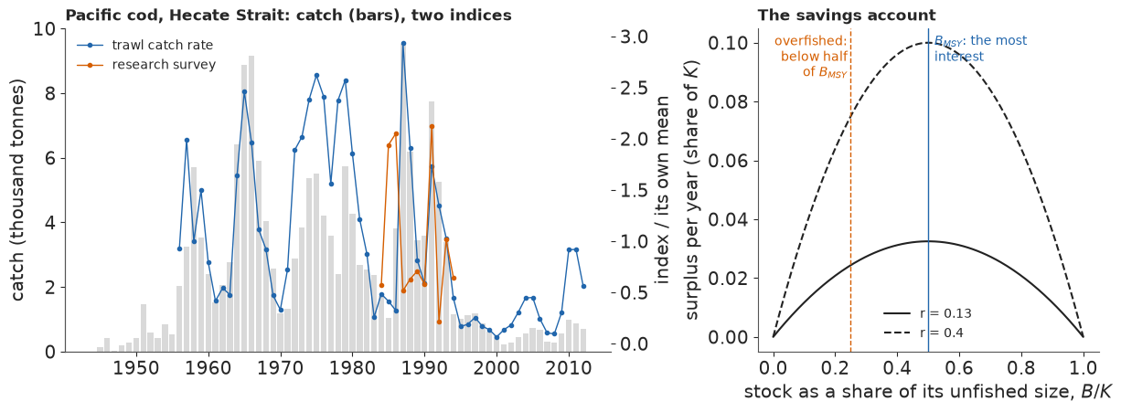
The catch peaked twice, at about 9,000 t in the mid-1960s and 9,500 t in 1987, and fell to a few hundred tonnes after 2000. The catch rate peaks in the 1970s and is lowest around 2000, with year-to-year jumps of a factor of two: observation error. The eleven-year survey does not obviously agree with it, and for 1944-1955 there is no index at all.
The right panel is the savings account: the surplus is a parabola in $B/K$ that peaks at half the unfished size whatever $r$ is; $r$ only sets the height. The dashed line is the usual "overfished" threshold, half of $B_{MSY}$.
B · A toy stock: what a one-way trip cannot tell
Two histories with a known truth
Before a real stock, a simulated one with $r = 0.4$, $K = 1{,}000$ t and so $MSY = 100$ t, an index with catchability $q = 0.001$ and 15% observation noise, and a little process noise. In the one-way trip the catch rises steadily from 10% to 150% of MSY over 40 years, and the stock declines from $K$ to about 40% of it. In the two-way trip the catch rises to 170% of MSY over 20 years and is then cut to 40%, so the stock falls and recovers. Hilborn & Walters (1992, Quantitative Fisheries Stock Assessment) made the point this toy illustrates: data from a fishery that has only ever gone down tell you little about how it would come back.
R_TRUE, K_TRUE, Q_TRUE, T_TOY = 0.4, 1000.0, 0.001, 40
MSY_TRUE = R_TRUE * K_TRUE / 4
tt = np.arange(T_TOY)
TRIPS = {"one-way trip": MSY_TRUE * (0.1 + 1.4 * tt / (T_TOY - 1)),
         "two-way trip": np.where(tt < 20, MSY_TRUE * (0.1 + 1.6 * tt / 19), 0.4 * MSY_TRUE)}
toy_rng = np.random.default_rng(1140)


def simulate(C, gen, sp=0.05, so=0.15):
    P = np.empty(len(C))
    P[0] = 1.0
    for k in range(1, len(C)):
        f = P[k - 1] + R_TRUE * P[k - 1] * (1 - P[k - 1]) - C[k - 1] / K_TRUE
        P[k] = max(f, 0.01) * np.exp(sp * gen.normal())
    return P, Q_TRUE * K_TRUE * P * np.exp(so * gen.normal(size=len(C)))


TOY = {k: (C,) + simulate(C, toy_rng) for k, C in TRIPS.items()}
for k, (C, P, I) in TOY.items():
    print(f"{k}: B/K from {P[0]:.2f} to a low of {P.min():.2f}, ending at {P[-1]:.2f}")
one-way trip: B/K from 1.00 to a low of 0.40, ending at 0.40
two-way trip: B/K from 1.00 to a low of 0.32, ending at 0.86
A fit with observation error only
The simplest fit, and the one fisheries scientists used for decades, ignores process error:
given $r$, $K$ and a start at $K$, the dynamics are deterministic, and only the index is noisy,
$\log I_t \sim N(\log q + \log B_t, \sigma_o)$. The recursion runs in pytensor.scan, and a
smooth floor $\epsilon \,\mathrm{softplus}(f/\epsilon)$ keeps the stock positive when a draw of
$(r, K)$ makes the catch larger than the fish. The priors are deliberately vague: $\log r \sim
N(\log 0.4, 1)$ and $K$ around five times the largest catch with a log sd of 1.
def toy_fit(C, I, seed=1):
    cmax = C.max()
    with pm.Model() as m:
        log_r = pm.Normal("log_r", np.log(0.4), 1.0)
        log_K = pm.Normal("log_K", np.log(5 * cmax), 1.0)
        r, K = pt.exp(log_r), pt.exp(log_K)

        def step(c, p, r, K):
            f = p + r * p * (1 - p) - c / K
            return 0.01 * pt.softplus(f / 0.01)

        Ps = pytensor.scan(step, sequences=[pt.as_tensor(C[:-1])],
                           outputs_info=[pt.constant(1.0, dtype="float64")],
                           non_sequences=[r, K], return_updates=False)
        P_all = pt.concatenate([pt.ones(1), Ps])
        lq = pm.Normal("log_qK", np.log(I).mean() - np.log(0.5), 2.0)
        so = pm.LogNormal("sigma_o", np.log(0.2), 0.5)
        pm.Normal("I", lq + pt.log(P_all), so, observed=np.log(I))
        return pm.sample(random_seed=seed, progressbar=False, target_accept=0.9)


t0 = time.time()
TOY_POST = {}
for k, (C, P, I) in TOY.items():
    idt = toy_fit(C, I)
    lr = idt.posterior["log_r"].values.ravel()
    lk = idt.posterior["log_K"].values.ravel()
    sm = az.summary(idt, var_names=["log_r", "log_K"], round_to=4)
    q_r, q_k, q_m = (np.quantile(v, [0.055, 0.5, 0.945])
                     for v in (np.exp(lr), np.exp(lk), np.exp(lr + lk) / 4))
    TOY_POST[k] = (lr, lk)
    print(f"{k}: divergences {int(idt.sample_stats['diverging'].sum())}, "
          f"max r_hat {sm.r_hat.max():.3f}, min ESS {sm.ess_bulk.min():.0f}, "
          f"corr(log r, log K) {np.corrcoef(lr, lk)[0, 1]:.2f}\n"
          f"   r {q_r[1]:.2f} ({q_r[0]:.2f}-{q_r[2]:.2f}), K {q_k[1]:,.0f} ({q_k[0]:,.0f}-"
          f"{q_k[2]:,.0f}), MSY {q_m[1]:.0f} ({q_m[0]:.0f}-{q_m[2]:.0f});  truth r 0.4, K 1,000, "
          f"MSY 100")
TIMES["toy"] = time.time() - t0
one-way trip: divergences 160, max r_hat 1.012, min ESS 186, corr(log r, log K) -0.99
   r 0.35 (0.10-1.08), K 1,213 (467-2,930), MSY 107 (69-128);  truth r 0.4, K 1,000, MSY 100
two-way trip: divergences 0, max r_hat 1.006, min ESS 727, corr(log r, log K) -0.98
   r 0.40 (0.33-0.49), K 971 (837-1,130), MSY 97 (91-103);  truth r 0.4, K 1,000, MSY 100
fig, axs = plt.subplots(2, 2, figsize=(11, 7.4), height_ratios=[1, 1.15])
for j, (k, (C, P, I)) in enumerate(TOY.items()):
    a = axs[0, j]
    a.bar(tt, C / MSY_TRUE, color=LIGHT, width=0.8)
    a.axhline(1, color=MUTED, lw=0.8, ls=":")
    a.text(0.5, 1.03, "catch = MSY", color=MUTED, fontsize=9.5)
    a.plot(tt, 2 * P, color=INK, lw=1.5, label="true B/B$_{MSY}$")
    a.plot(tt, 2 * I / (Q_TRUE * K_TRUE), "o", color=HI, ms=3.5, label="index (scaled)")
    a.set_ylim(0, 2.3)
    a.set_title(f"{k}; bars: catch / MSY", loc="left", fontsize=11.5)
    a.legend(loc="upper right", fontsize=9.5)
    lr, lk = TOY_POST[k]
    b = axs[1, j]
    b.scatter(np.exp(lr[::2]), np.exp(lk[::2]), s=3, alpha=0.25, color=HI)
    b.plot(R_TRUE, K_TRUE, "*", color=LO, ms=15, label="truth")
    rg = np.geomspace(0.05, 3, 50)
    b.plot(rg, 4 * MSY_TRUE / rg, color=MUTED, lw=0.8, ls="--", label="r K / 4 = 100 (true MSY)")
    b.set_xscale("log")
    b.set_yscale("log")
    b.set_xlim(0.08, 1.5)
    b.set_ylim(300, 6000)
    b.set_xlabel("r")
    b.set_ylabel("K (t)")
    b.legend(loc="upper right", fontsize=9.5)
    b.set_title(f"posterior draws, corr(log r, log K) {np.corrcoef(lr, lk)[0, 1]:.2f}",
                loc="left", fontsize=11.5)
fig.suptitle("A one-way trip leaves r and K on a thin ridge; a recovery pins them down",
             x=0.01, ha="left", fontsize=13);
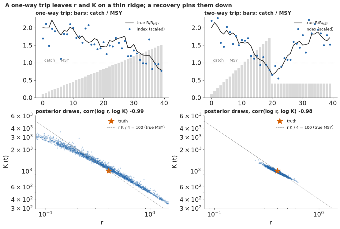
On the one-way trip the posterior is a long, thin banana: $\log r$ and $\log K$ are correlated at $-0.99$, and $r$ could be anything from 0.1 to 1.1 a year, with $K$ moving the other way from about 470 to 2,900 t. The data fix one combination, roughly the surplus the stock produced while it declined (MSY 69-128 t), and say almost nothing about whether that is a fast growth rate on a small stock or a slow one on a big stock. The 160 divergences come from the ends of the banana, where it bends and narrows.
On the two-way trip the recovery after the cut is the missing experiment: how fast the stock came back measures $r$, and the ridge shrinks to a short segment around the truth ($r$ 0.33-0.49, MSY 91-103 t, no divergences). Real fisheries are mostly one-way trips, so information about $r$ has to come from biology and from other stocks of the same kind. That is what part D does.
C · One real stock in PyMC
The state-space model
For stock $s$ we work with the depletion $P_{st} = B_{st}/K_s$ and with catches divided by the stock's largest catch $\bar C_s$, so that $K_s$ is in units of the largest catch and every stock has the same scale. The model, after Meyer & Millar (1999), is
$$f_{st} = P_{s,t-1} + r_s P_{s,t-1}(1 - P_{s,t-1}) - C_{s,t-1}/K_s, \qquad \log P_{st} \sim N\big(\log \tilde f_{st},\ \sigma_p\big),$$
$$\log I_{it} \sim N\big(\log (qK)_i + \log P_{s(i),t},\ \sigma_{o,i}\big),$$
where $\tilde f = \epsilon\,\mathrm{softplus}(f/\epsilon)$ is a smooth floor at about $\epsilon = 1\%$ of $K$, and $i$ runs over the index series (Pacific cod in Hecate Strait has two). A stock cannot lose more fish than it has, so a penalty $-\sum \mathrm{softplus}\big((0.02 - f_{st})/0.005\big)$ removes draws in which the catch would take the stock below 2% of $K$; without it the floor alone would let a tiny $K$ explain any catch. The priors:
- $\log P_{s1} \sim N(\log 0.8, 0.3)$: lightly fished when the record starts, an assumption that flatters records starting after heavy fishing (Scotian Shelf silver hake from 1977, after the distant-water fleets; Chilean hake's catches here from 1968);
- $\log K_s \sim N(\log 5, 0.8)$ in units of the largest catch: about 1.4 to 18 times it (89%);
- $\log r_s \sim N(m_s, w_s)$ with $m_s$ the log midpoint of the FishBase-CMSY range and $w_s$ a quarter of its log width, so the range is a 95% interval (part D keeps the centre and changes the width);
- $\sigma_p \sim \mathrm{LogNormal}(\log 0.1, 0.5)$, $\sigma_{o,i} \sim \mathrm{LogNormal}(\log 0.25, 0.5)$, and $\log(qK)_i$ vague around the index's mean.
The states $\log P_{st}$ are free parameters (pm.Flat), and the process and initial
densities enter as pm.Potential terms: the centred form. The non-centred form, usually
recommended for hierarchical models, pushes standardised innovations through a scan; we try it
too. One helper flattens any list of stocks into stock-year arrays, and one builds the model.
def prep(stocks, source=RAM, use_index=True, multi_only=True):
    """Flatten stock-years for several stocks; catches in units of each stock's largest catch."""
    st, years, C, first, prev, cmax, m_r, s_r, fam = [], [], [], [], [], [], [], [], []
    obs_state, obs_ser, logI, ser_name, ser_m, ser_stock = [], [], [], [], [], []
    off = 0
    for s, sid in enumerate(stocks):
        g = source[source.stockid == sid].sort_values("year").reset_index(drop=True)
        T = len(g)
        cmax.append(g.catch_t.max())
        st += [s] * T
        years += list(g.year)
        C += list(g.catch_t / g.catch_t.max())
        first.append(off)
        prev += list(range(off, off + T - 1))
        lo, hi = g.r_lo.iloc[0], g.r_hi.iloc[0]
        m_r.append(0.5 * (np.log(lo) + np.log(hi)))
        s_r.append((np.log(hi) - np.log(lo)) / 4)
        fam.append(g.family.iloc[0])
        for kind in ("cpue", "survey") if use_index else ():
            ok = (g[kind].notna() & (g[kind] > 0)).to_numpy()
            if ok.sum() >= 5:
                li = np.log(g[kind][ok].to_numpy())
                obs_state += list(off + np.where(ok)[0])
                obs_ser += [len(ser_name)] * int(ok.sum())
                logI += list(li)
                ser_name.append(f"{sid}:{kind}")
                ser_m.append(li.mean())
                ser_stock.append(s)
        off += T
    if multi_only:  # family effects only for families with two or more stocks
        fam = [f if fam.count(f) >= 2 else "(single)" for f in fam]
    fams = sorted(set(fam))
    st = np.array(st)
    first = np.array(first)
    last = np.r_[first[1:] - 1, off - 1]
    return dict(stocks=list(stocks), S=len(stocks), N=off, st=st, years=np.array(years),
                C=np.array(C), first=first, last=last, rest=np.setdiff1d(np.arange(off), first),
                prev=np.array(prev), cmax=np.array(cmax), obs_state=np.array(obs_state, int),
                obs_ser=np.array(obs_ser, int), logI=np.array(logI), ser_name=ser_name,
                ser_m=np.array(ser_m), ser_stock=np.array(ser_stock, int), m_r=np.array(m_r),
                s_r=np.array(s_r), fam_names=fams, fam=np.array([fams.index(f) for f in fam]))


def ss_model(d, *, hier=False, sigma_p="stock", sp_mu=np.log(0.1), sp_sd=0.5, k_mu=np.log(5.0),
             k_sd=0.8, eps=0.01, pen=0.005, floor=0.02, end_prior=None):
    """Schaefer state-space model with centred free states (Meyer & Millar 1999).

    sigma_p: "stock" (one per stock), "pooled" (one for all) or a number (fixed).
    end_prior: (lo, hi) range for the final depletion B/K, imposed as a steep wall (CMSY's filter).
    """
    coords = {"stock": d["stocks"], "state": np.arange(d["N"]), "series": d["ser_name"],
              "family": d["fam_names"]}
    st, prev, rest, first = d["st"], d["prev"], d["rest"], d["first"]
    with pm.Model(coords=coords) as m:
        if hier:
            sigma_fam = pm.HalfNormal("sigma_fam", 0.4)
            tau_r = pm.HalfNormal("tau_r", 0.4)
            w = pm.Normal("w_fam", 0, 1, dims="family")
            z = pm.Normal("z_r", 0, 1, dims="stock")
            fe = sigma_fam * w
            if "(single)" in d["fam_names"]:
                fe = pt.set_subtensor(fe[d["fam_names"].index("(single)")], 0.0)
            log_r = pm.Deterministic("log_r", d["m_r"] + fe[d["fam"]] + tau_r * z, dims="stock")
        else:
            log_r = pm.Normal("log_r", d["m_r"], d["s_r"], dims="stock")
        r = pm.Deterministic("r", pt.exp(log_r), dims="stock")
        log_K = pm.Normal("log_K", k_mu, k_sd, dims="stock")
        K = pt.exp(log_K)
        if sigma_p == "pooled":
            sp = pm.LogNormal("sigma_p", sp_mu, sp_sd) * pt.ones(d["S"])
        elif sigma_p == "stock":
            sp = pm.LogNormal("sigma_p", sp_mu, sp_sd, dims="stock")
        else:
            sp = pt.as_tensor(np.full(d["S"], float(sigma_p)))
        logP = pm.Flat("logP", dims="state")
        Pp = pt.exp(logP)[prev]
        f = Pp + r[st[rest]] * Pp * (1 - Pp) - d["C"][prev] / K[st[rest]]
        f_pos = eps * pt.softplus(f / eps)
        pm.Potential("start", pm.logp(pm.Normal.dist(np.log(0.8), 0.3), logP[first]).sum())
        pm.Potential("process", pm.logp(pm.Normal.dist(pt.log(f_pos), sp[st[rest]]),
                                        logP[rest]).sum())
        pm.Potential("feasible", -pt.softplus((floor - f) / pen).sum())
        if end_prior is not None:
            lo, hi = np.log(end_prior[0]), np.log(end_prior[1])
            lpl = logP[d["last"]]  # log-density falls by 20 per unit of log B/K outside the range
            pm.Potential("end_prior", (-pt.softplus((lpl - hi) / 0.05)
                                       - pt.softplus((lo - lpl) / 0.05)).sum())
        if d["ser_name"]:
            lq = pm.Normal("log_qK", d["ser_m"] - np.log(0.5), 2.0, dims="series")
            sigma_o = pm.LogNormal("sigma_o", np.log(0.25), 0.5, dims="series")
            pm.Normal("logI", lq[d["obs_ser"]] + logP[d["obs_state"]], sigma_o[d["obs_ser"]],
                      observed=d["logI"])
    return m


def sample(m, d, seed, ta=0.9, **kw):
    t0 = time.time()
    idata = pm.sample(model=m, random_seed=seed, target_accept=ta, progressbar=False,
                      initvals={"logP": np.full(d["N"], np.log(0.5))}, **kw)
    return idata, time.time() - t0


def draws(idata, v):
    """Posterior draws as an array (draw, ...), chains stacked."""
    return idata.posterior[v].stack(s=("chain", "draw")).transpose("s", ...).values


def status(idata, d):
    """B/B_MSY = 2P and F/F_MSY = (C/B)/(r/2) for every stock-year and draw."""
    P = np.exp(draws(idata, "logP"))
    r, K = draws(idata, "r")[:, d["st"]], np.exp(draws(idata, "log_K"))[:, d["st"]]
    return 2 * P, d["C"][None, :] / (K * P) / (r / 2)


def report(idata, d, names, label, secs):
    div = int(idata.sample_stats["diverging"].sum())
    sm = pd.concat([az.summary(idata, var_names=[v], round_to=4) for v in names])
    print(f"{label}: {secs:.0f} s, {div} divergences of {idata.posterior.sizes['draw'] * 4:,}, "
          f"max r_hat {sm.r_hat.max():.3f}, min bulk ESS {sm.ess_bulk.min():.0f}, min tail ESS "
          f"{sm.ess_tail.min():.0f} (warm-up {idata.posterior.attrs.get('tuning_steps')})")
    return div


D1 = prep(["PCODHS"], multi_only=False)
print(f"{D1['N']} states, {len(D1['logI'])} index values in {len(D1['ser_name'])} series; "
      f"prior r 95% range {np.exp(D1['m_r'][0] - 2 * D1['s_r'][0]):.2f}-"
      f"{np.exp(D1['m_r'][0] + 2 * D1['s_r'][0]):.2f}")
69 states, 68 index values in 2 series; prior r 95% range 0.05-0.50
The prior, checked by simulation
Because the dynamics are potentials, PyMC cannot draw a prior predictive for us, so we simulate it in NumPy: draw $r$, $K$, $\sigma_p$ and the start from their priors, run Pacific cod's real catches through the dynamics, and look at the biomass paths. A sensible prior should allow stocks from barely touched to heavily fished, and should not make most stocks collapse under the catches that were actually taken.
def prior_paths(d, n, gen, eps=0.01, k_mu=np.log(5.0), k_sd=0.8):
    r = np.exp(gen.normal(d["m_r"][0], d["s_r"][0], n))
    K = np.exp(gen.normal(k_mu, k_sd, n))
    sp = np.exp(gen.normal(np.log(0.1), 0.5, n))
    P = np.empty((n, d["N"]))
    P[:, 0] = np.exp(gen.normal(np.log(0.8), 0.3, n))
    fmin = np.full(n, np.inf)
    for t in range(1, d["N"]):
        f = P[:, t - 1] + r * P[:, t - 1] * (1 - P[:, t - 1]) - d["C"][t - 1] / K
        fmin = np.minimum(fmin, f)
        P[:, t] = eps * np.logaddexp(0, f / eps) * np.exp(sp * gen.normal(size=n))
    return 2 * P, K, fmin


BB_PRIOR, K_PRIOR, FMIN = prior_paths(D1, 4000, np.random.default_rng(7))
crash = FMIN < 0.02
print(f"K in tonnes, 89% prior range: {np.quantile(K_PRIOR, 0.055) * D1['cmax'][0]:,.0f}-"
      f"{np.quantile(K_PRIOR, 0.945) * D1['cmax'][0]:,.0f} (largest catch "
      f"{D1['cmax'][0]:,.0f} t)")
print(f"prior paths in which the catch would empty the stock: {crash.mean():.0%} "
      f"(the feasibility penalty removes them)")
print(f"surviving paths: final B/B_MSY median {np.median(BB_PRIOR[~crash, -1]):.2f}, "
      f"89% {np.quantile(BB_PRIOR[~crash, -1], 0.055):.2f}-"
      f"{np.quantile(BB_PRIOR[~crash, -1], 0.945):.2f}")
fig, ax = plt.subplots(figsize=(10, 4))
yrs1 = D1["years"]
for i in np.where(~crash)[0][:40]:
    ax.plot(yrs1, BB_PRIOR[i], color=HI, alpha=0.25, lw=0.9)
for i in np.where(crash)[0][:10]:
    ax.plot(yrs1, BB_PRIOR[i], color=LO, alpha=0.5, lw=0.9)
ax.axhline(1, color=INK, lw=1)
ax.set_ylim(0, 4)
ax.set_ylabel("B / B$_{MSY}$")
ax.set_title(wrap(f"Prior paths for Pacific cod under its real catches: 40 that survive (blue) "
                  f"and 10 of the {crash.mean():.0%} in which the catch empties the stock "
                  f"(vermilion)", 95), loc="left");
K in tonnes, 89% prior range: 13,138-162,694 (largest catch 9,540 t)
prior paths in which the catch would empty the stock: 71% (the feasibility penalty removes them)
surviving paths: final B/B_MSY median 1.83, 89% 0.93-2.48
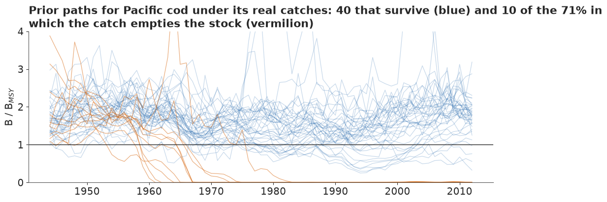
The prior allows $K$ from about 1.4 to 18 times the largest catch (13,000 to 163,000 t in this simulation), yet about 70% of the prior draws cannot support the catches that were taken: with a growth rate near 0.16, a stock five times the largest catch has an MSY of only a fifth of it, and Pacific cod was fished near its largest catch for years.
The prior that reaches the data is the surviving 30%, and it has an opinion: those paths mostly end above the healthy level (final B/BMSY median about 1.8, 89% range 0.9-2.5), because a stock big enough to survive the catches was never heavily depleted by them. An index can overrule that opinion. Without one, in part F, it is the answer.
Failure 1: non-centred states
The usual advice for a hierarchical model with a poorly identified scale is to non-centre:
sample standardised innovations $e_t \sim N(0, 1)$ and build the states as
$\log P_t = \log \tilde f_t + \sigma_p e_t$ in a scan. We try that first, with a short run.
def nc_model(d, eps=0.01):
    """Non-centred single-stock version: innovations through a scan recursion."""
    T = d["N"]
    with pm.Model() as m:
        log_r = pm.Normal("log_r", d["m_r"][0], d["s_r"][0])
        r = pm.Deterministic("r", pt.exp(log_r))
        log_K = pm.Normal("log_K", np.log(5.0), 0.8)
        K = pt.exp(log_K)
        sp = pm.LogNormal("sigma_p", np.log(0.1), 0.5)
        e0 = pm.Normal("e0", 0, 1)
        e = pm.Normal("e", 0, 1, shape=T - 1)

        def step(e_t, c_t, lp, r, K, sp):
            p = pt.exp(lp)
            f = p + r * p * (1 - p) - c_t / K
            return pt.log(eps * pt.softplus(f / eps)) + sp * e_t, f

        lps, fs = pytensor.scan(step, sequences=[e, pt.as_tensor(d["C"][:-1])],
                                outputs_info=[np.log(0.8) + 0.3 * e0, None],
                                non_sequences=[r, K, sp], return_updates=False)
        logP = pm.Deterministic("logP", pt.concatenate([(np.log(0.8) + 0.3 * e0)[None], lps]))
        pm.Potential("feasible", -pt.softplus((0.02 - fs) / 0.005).sum())
        lq = pm.Normal("log_qK", d["ser_m"] - np.log(0.5), 2.0, shape=len(d["ser_name"]))
        so = pm.LogNormal("sigma_o", np.log(0.25), 0.5, shape=len(d["ser_name"]))
        pm.Normal("logI", lq[d["obs_ser"]] + logP[d["obs_state"]], so[d["obs_ser"]],
                  observed=d["logI"])
    return m


t0 = time.time()
id_nc = pm.sample(model=nc_model(D1), random_seed=RANDOM_SEED, target_accept=0.95, tune=400,
                  draws=500, progressbar=False)
DIV_NC = report(id_nc, D1, ["log_r", "log_K", "sigma_p"], "non-centred, Pacific cod",
                time.time() - t0)
TIMES["non-centred"] = time.time() - t0
del id_nc
non-centred, Pacific cod: 44 s, 194 divergences of 2,000, max r_hat 1.556, min bulk ESS 7, min tail ESS 7 (warm-up 400)
About one transition in ten diverges, r_hat reaches 1.6 and the worst bulk ESS is 7: the chains have not mixed. The reason is the one E46 met with a chaotic map. Every state depends on every earlier innovation through the nonlinear dynamics, so a small change in $r$ or an early $e_t$ moves the whole path, while the index pins each $\log P_t$ tightly: a curved, narrow tube in the innovations that no single step size can follow. Non-centring helps when the data are weak about each state; here they are strong.
The centred fit
id1, secs = sample(ss_model(D1), D1, RANDOM_SEED, ta=0.95)
DIV_C1 = report(id1, D1, ["log_r", "log_K", "sigma_p", "sigma_o", "logP"],
                "centred, Pacific cod", secs)
TIMES["centred"] = secs
dv = id1.sample_stats["diverging"].stack(s=("chain", "draw")).values
sp1 = draws(id1, "sigma_p").ravel()
print(f"sigma_p: median {np.median(sp1):.3f}; in divergent draws "
      f"{np.median(sp1[dv]) if dv.any() else float('nan'):.3f}")
print(f"r: prior median {np.exp(D1['m_r'][0]):.2f}, posterior median "
      f"{np.median(draws(id1, 'r')):.2f}")
centred, Pacific cod: 3 s, 28 divergences of 4,000, max r_hat 1.071, min bulk ESS 40, min tail ESS 55 (warm-up 400)
sigma_p: median 0.400; in divergent draws 0.523
r: prior median 0.16, posterior median 0.15
With free states the same stock samples in a few seconds, and the worst r_hat drops from 1.6 to about 1.07. That is better, not clean: a few dozen divergences remain, the lowest ESS is about 40, and the divergent draws have a larger process noise than the rest (median about 0.52 against 0.40). This is not the familiar funnel at a scale near zero. When $\sigma_p$ is large, the 12 years before the first index (1944-1955) are free to wander, and the posterior gets a thin, wide-spreading region that the sampler cannot enter smoothly. We will come back to it.
The fit should first reproduce what it was fitted to. The posterior predictive for each index is the fitted state times the catchability with fresh observation noise.
lp1, lq1, so1 = draws(id1, "logP"), draws(id1, "log_qK"), draws(id1, "sigma_o")
pp_rng = np.random.default_rng(3)
fig, axs = plt.subplots(1, 2, figsize=(12, 3.8))
for i, (a, nm) in enumerate(zip(axs, D1["ser_name"])):
    sel = D1["obs_ser"] == i
    stt = D1["obs_state"][sel]
    rep = lq1[:, [i]] + lp1[:, stt] + so1[:, [i]] * pp_rng.normal(size=(len(lq1), sel.sum()))
    lo_, hi_ = np.quantile(rep, [0.055, 0.945], axis=0)
    a.fill_between(D1["years"][stt], np.exp(lo_), np.exp(hi_), color=HI, alpha=0.25, lw=0,
                   label="89% predictive")
    a.plot(D1["years"][stt], np.exp(D1["logI"][sel]), "o", color=INK, ms=3.5, label="observed")
    inside = ((D1["logI"][sel] >= lo_) & (D1["logI"][sel] <= hi_)).mean()
    a.set_yscale("log")
    a.legend(fontsize=9.5)
    a.set_title(f"{nm.split(':')[1]}: {inside:.0%} of {sel.sum()} values inside the 89% band",
                loc="left")
    print(f"{nm}: {inside:.0%} inside; sigma_o median {np.median(so1[:, i]):.2f}")
PCODHS:cpue: 100% inside; sigma_o median 0.40
PCODHS:survey: 91% inside; sigma_o median 0.72
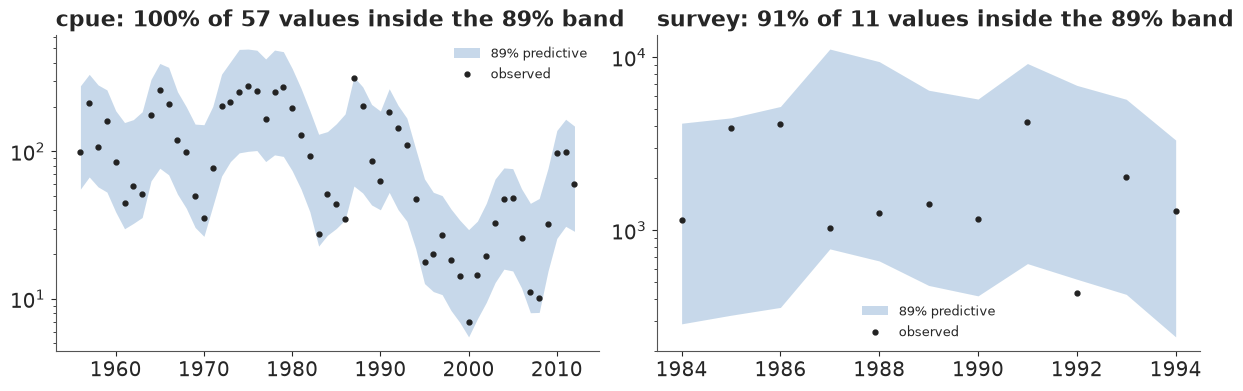
All 57 catch-rate values and 10 of the 11 survey values sit inside their 89% predictive bands, if anything too good. The catch rate gets an observation sd of about 0.4 and the short survey about 0.7: the survey disagrees with the catch rate in the late 1980s and the model trusts the longer series. This check cannot fail very badly in a state-space model, because the states can follow the index wherever the process noise allows.
The data barely move $r$ (posterior median 0.15, prior 0.16): like the toy's one-way trip, the index says how the stock went down and partly back up, not how fast it grows.
Failure 2: a long record with no index
Georges Bank yellowtail flounder has 80 years of catch (from 1935) but a survey only from 1987, so for half a century the states are tied only to the catches and the dynamics. Fitted alone with its own process noise:
DG = prep(["YELLGB"], multi_only=False)
idg, secs = sample(ss_model(DG), DG, RANDOM_SEED, ta=0.95)
DIV_G = report(idg, DG, ["log_r", "log_K", "sigma_p", "logP"], "Georges Bank yellowtail alone",
               secs)
dv = idg.sample_stats["diverging"].stack(s=("chain", "draw")).values
spg = draws(idg, "sigma_p").ravel()
print(f"sigma_p: median {np.median(spg):.3f}, 89% {np.quantile(spg, 0.055):.3f}-"
      f"{np.quantile(spg, 0.945):.3f}; in divergent draws {np.median(spg[dv]):.3f}")
TIMES["yellowtail alone"] = secs
del idg
Georges Bank yellowtail alone: 5 s, 298 divergences of 4,000, max r_hat 1.024, min bulk ESS 270, min tail ESS 313 (warm-up 400)
sigma_p: median 0.540, 89% 0.377-0.737; in divergent draws 0.682
About 300 divergences. The process sd comes out at about 0.54 (89% 0.38-0.74), more than for Pacific cod, and the divergent draws again sit at its upper end (median about 0.68), where five decades of index-free states can roam. One stock cannot tell how big its own process noise is when most of its states are unobserved; part D lets the stocks share it.
D · Eighteen stocks, shared biology
What the stocks share
Two things are pooled. First, growth. The prior for each stock's $\log r$ is centred at the midpoint of its resilience range, and stocks of the same family share a family effect:
$$\log r_s = m_s + \sigma_{fam}\, w_{f(s)} + \tau_r\, z_s, \qquad w, z \sim N(0, 1),\quad \sigma_{fam}, \tau_r \sim \mathrm{HalfNormal}(0.4).$$
Only cod, flatfish and hake have more than one stock here. A family effect for a family with a single stock cannot be told apart from that stock's own effect: the data see only their sum, and in our trial fits that unidentified pair added divergences. So the six single-stock families get no family term.
Second, process noise. Good and bad years differ between stocks, but their typical size may be similar enough for one shared $\sigma_p$, which lets the stocks with long index records inform those with long gaps (part C showed that a stock's own noise is poorly learned there). We fit the 18 stocks both ways, first with one $\sigma_p$ per stock (a short run of 250 draws per chain), then with one shared value. The model has 1,030 latent states, 21 index series with 728 values, and about 80 other parameters.
MAIN = ["PCODHS", "PCODWCVANI", "PCOD5AB", "RSOLE5AB", "RSOLEHSTR", "YELL3LNO", "YELLGB",
        "WITFLOUN4RST", "SPHAKECH", "SHAKE4VWX", "SHAKESGBMATL", "SHAKEGOMNGB", "REDFISHSPP3LN",
        "NZSNAPNZ7", "TREVALLYTRE7", "NZLINGESE", "BLSHARNPAC", "WHAKE4T"]
D = prep(MAIN)
print(f"{D['S']} stocks, {D['N']:,} states, {len(D['ser_name'])} series, "
      f"{len(D['logI'])} index values; families with a shared effect: "
      f"{[f for f in D['fam_names'] if f != '(single)']}")
MAIN_VARS = ["r", "log_K", "sigma_p", "sigma_o", "log_qK", "sigma_fam", "tau_r", "w_fam", "z_r",
             "logP"]
id_ps, secs = sample(ss_model(D, hier=True, sigma_p="stock"), D, RANDOM_SEED, ta=0.9, draws=250)
TIMES["18 stocks, per-stock noise"] = secs
DIV_PS = report(id_ps, D, MAIN_VARS, "18 stocks, per-stock process noise", secs)
dep_ps = id_ps.sample_stats["depth"].values
dv_ps = id_ps.sample_stats["diverging"].stack(s=("chain", "draw")).values
sp_ps = draws(id_ps, "sigma_p")
jg = MAIN.index("YELLGB")
print(f"tree depth 10 in {(dep_ps >= 10).mean():.0%} of draws; Georges Bank yellowtail sigma_p "
      f"median {np.median(sp_ps[:, jg]):.2f}, in divergent draws "
      f"{np.median(sp_ps[dv_ps, jg]):.2f}; per-stock medians {np.median(sp_ps, 0).min():.2f}-"
      f"{np.median(sp_ps, 0).max():.2f}")
del id_ps
18 stocks, 1,030 states, 21 series, 728 index values; families with a shared effect: ['Gadidae', 'Merlucciidae', 'Pleuronectidae']
18 stocks, per-stock process noise: 53 s, 114 divergences of 1,000, max r_hat 1.131, min bulk ESS 30, min tail ESS 40 (warm-up 400)
tree depth 10 in 55% of draws; Georges Bank yellowtail sigma_p median 0.54, in divergent draws 0.62; per-stock medians 0.08-0.54
Per-stock noise fails: more than one draw in ten diverges, r_hat reaches about 1.13, and over half the transitions hit nutpie's maximum tree depth of 10. The stocks' own noise estimates range from about 0.1 to 0.55, and Georges Bank yellowtail again sits at the top, with its divergent draws higher still. That spread suggests the noise really does differ between stocks, so a shared value trades some bias for a model that samples; its prior, centred at 0.1, also sits well below where the stocks will put it. Now the shared value:
M_MAIN = ss_model(D, hier=True, sigma_p="pooled")
id_main, secs = sample(M_MAIN, D, RANDOM_SEED, ta=0.9)
TIMES["18 stocks"] = secs
DIV_MAIN = report(id_main, D, MAIN_VARS, "18 stocks, shared process noise", secs)
SP = draws(id_main, "sigma_p").ravel()
print(f"shared process sd {np.median(SP):.3f} (89% {np.quantile(SP, 0.055):.3f}-"
      f"{np.quantile(SP, 0.945):.3f}); sigma_fam {np.median(draws(id_main, 'sigma_fam')):.2f}, "
      f"tau_r {np.median(draws(id_main, 'tau_r')):.2f}")
dep = id_main.sample_stats["depth"].values
print(f"tree depth: mean {dep.mean():.1f}, max {dep.max()}, at depth 10 in "
      f"{int((dep >= 10).sum())} draws ({(dep >= 10).mean():.1%})")
dv_m = id_main.sample_stats["diverging"].stack(s=("chain", "draw")).values
r_m = draws(id_main, "r")
top10 = (r_m[dv_m] > np.quantile(r_m, 0.9, axis=0)).mean(axis=0)  # per stock, among divergent draws
for s in np.argsort(top10)[::-1][:3]:
    print(f"{NICE[MAIN[s]]}: {top10[s]:.0%} of the divergent draws in the top tenth of its r "
          f"(median r {np.median(r_m[dv_m, s]):.2f} in them, {np.median(r_m[:, s]):.2f} overall)")
18 stocks, shared process noise: 48 s, 11 divergences of 4,000, max r_hat 1.016, min bulk ESS 308, min tail ESS 312 (warm-up 400)
shared process sd 0.236 (89% 0.211-0.264); sigma_fam 0.43, tau_r 0.30
tree depth: mean 7.2, max 10, at depth 10 in 1 draws (0.0%)
Trevally, New Zealand (TRE 7): 64% of the divergent draws in the top tenth of its r (median r 0.36 in them, 0.17 overall)
Ling, SE Australia: 45% of the divergent draws in the top tenth of its r (median r 0.23 in them, 0.16 overall)
Rock sole, Queen Charlotte Sound: 36% of the divergent draws in the top tenth of its r (median r 0.18 in them, 0.17 overall)
About ten divergences out of 4,000 draws remain, against 114 in 1,000 with per-stock noise. r_hat is at most about 1.02, every parameter and state has at least about 300 effective draws in the bulk and in the tails, a single draw reached the maximum tree depth of 10 (more than half did with per-stock noise), and the fit takes under a minute. The divergent draws sit in the upper tail of trevally's growth rate: about two thirds of them are in its top tenth, with a median $r$ of about 0.36 against 0.17 overall. That is few enough to report and move on, not few enough to ignore: the posterior has a corner the sampler visits reluctantly.
The shared process sd comes out at about 0.24: a typical stock departs from the Schaefer prediction by about a quarter each year. Part of that is real (recruitment varies by factors of several), and part is everything a logistic curve leaves out: age structure, changing selectivity, a changing environment.
Does the 18-stock fit reproduce its indices?
The same predictive check as for Pacific cod, now for all 21 index series: the share of each series' values inside its 89% posterior predictive band, and the worst series drawn out.
LP_M, LQ_M, SO_M = draws(id_main, "logP"), draws(id_main, "log_qK"), draws(id_main, "sigma_o")
ppc_rng = np.random.default_rng(5)
sub = ppc_rng.choice(LP_M.shape[0], 1000, replace=False)
os_, oi_ = D["obs_ser"], D["obs_state"]
REP = (LQ_M[sub][:, os_] + LP_M[sub][:, oi_]
       + SO_M[sub][:, os_] * ppc_rng.normal(size=(len(sub), len(os_))))
lo_m, hi_m = np.quantile(REP, [0.055, 0.945], axis=0)
inside_m = (D["logI"] >= lo_m) & (D["logI"] <= hi_m)
PPC = pd.DataFrame({"series": [f"{NICE[n.split(':')[0]]}: {n.split(':')[1]}"
                               for n in D["ser_name"]],
                    "values": np.bincount(os_),
                    "inside_89": np.bincount(os_, inside_m) / np.bincount(os_),
                    "sigma_o": np.median(SO_M, 0)}).set_index("series").sort_values("inside_89")
print(PPC.round(2).to_string())
print(f"\nall series: {inside_m.mean():.0%} of {len(inside_m)} values inside their 89% band; "
      f"series below 80%: {int((PPC.inside_89 < 0.8).sum())}")
worst = int(np.argmin(np.bincount(os_, inside_m) / np.bincount(os_)))
w_sel = os_ == worst
fig, ax = plt.subplots(figsize=(10, 3.6))
ax.fill_between(D["years"][oi_[w_sel]], np.exp(lo_m[w_sel]), np.exp(hi_m[w_sel]), color=HI,
                alpha=0.25, lw=0, label="89% predictive")
ax.plot(D["years"][oi_[w_sel]], np.exp(np.median(REP[:, w_sel], 0)), color=HI, lw=1.2,
        label="predictive median")
ax.plot(D["years"][oi_[w_sel]], np.exp(D["logI"][w_sel]), "o", color=INK, ms=3.5, label="observed")
ax.set_yscale("log")
ax.legend(fontsize=9.5)
ax.set_title(wrap(f"Worst-covered series, {PPC.index[0]}: {PPC.inside_89.iloc[0]:.0%} of "
                  f"{PPC['values'].iloc[0]} values inside the 89% band", 70), loc="left");
del LP_M, REP
                                                 values  inside_89  sigma_o
series
Yellowtail flounder, Georges Bank: survey            28       0.86     0.83
Pacific cod, Hecate Strait: survey                   11       0.91     0.63
Pacific cod, Hecate Strait: cpue                     57       0.93     0.55
White hake, S. Gulf of St Lawrence: survey           39       0.95     0.39
Silver hake, Gulf of Maine: cpue                     47       0.96     0.36
Pacific cod, W. Vancouver Island: cpue               46       0.98     0.33
Pacific cod, Queen Charlotte Sound: cpue             57       0.98     0.33
Rock sole, Queen Charlotte Sound: cpue               47       1.00     0.10
Rock sole, Hecate Strait: survey                     12       1.00     0.35
Rock sole, Hecate Strait: cpue                       52       1.00     0.13
Witch flounder, Gulf of St Lawrence: survey          41       1.00     0.38
Yellowtail flounder, Grand Banks: cpue               45       1.00     0.08
Hake, Chile: cpue                                    31       1.00     0.16
Silver hake, Scotian Shelf: survey                   38       1.00     0.38
Silver hake, S. Georges Bank-Mid-Atlantic: cpue      47       1.00     0.29
Rock sole, Queen Charlotte Sound: survey              7       1.00     0.31
Redfish, Grand Banks: cpue                           36       1.00     0.11
Snapper, New Zealand (SNA 7): cpue                   25       1.00     0.31
Ling, SE Australia: cpue                             21       1.00     0.10
Trevally, New Zealand (TRE 7): cpue                  23       1.00     0.12
Blue shark, North Pacific: cpue                      18       1.00     0.10

all series: 98% of 728 values inside their 89% band; series below 80%: 0
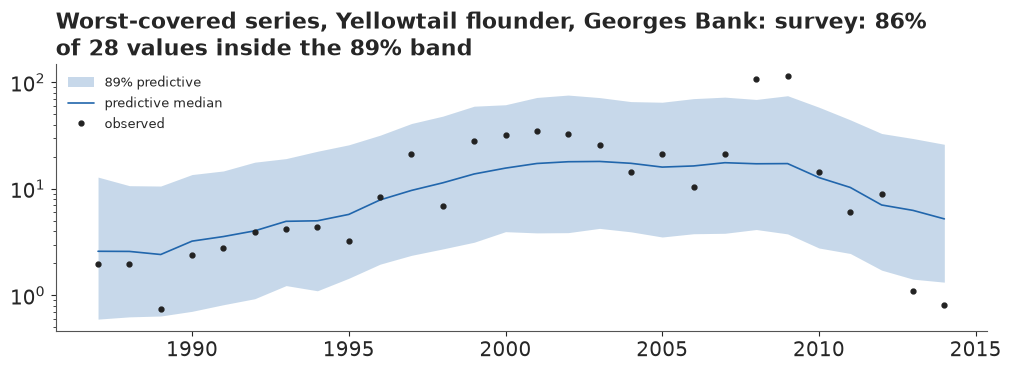
Of the 728 index values, 98% fall inside their 89% bands, more than the nominal 89% because the states are free to follow each index, the same leniency as for Pacific cod. No series falls below 80%. The worst, Georges Bank yellowtail's survey (86%), has the largest observation sd (about 0.8). Two isolated spikes, 107 and 115 kg per tow in 2008-09 against 21 in 2007 and 15 in 2010, sit above the band; they look like outliers, and they inflate that sd. The last two values, 2013-14, about a hundredth of the spikes, sit well below it: so noisy a survey lets the model treat the final collapse partly as noise. Part E tests both. The check cannot say whether the dynamics are right; the official assessments test that below.
How much did the data teach us about growth?
For each stock we compare the prior and posterior of $\log r$. The prior here is the hierarchical one, simulated in NumPy from the same half-normal scales. The contraction is $1 - \mathrm{var}_{post}/\mathrm{var}_{prior}$: 0 means the data taught nothing, 1 that they settled it.
DRAW = {v: draws(id_main, v) for v in ("r", "log_K")}
BB, UU = status(id_main, D)
pr_rng = np.random.default_rng(11)
n_pr = 20000
sf_pr, tr_pr = np.abs(pr_rng.normal(0, 0.4, n_pr)), np.abs(pr_rng.normal(0, 0.4, n_pr))
LOGR_PRIOR = {}
rows = []
for s, sid in enumerate(MAIN):
    single = D["fam_names"][D["fam"][s]] == "(single)"
    pl = (D["m_r"][s] + (0 if single else sf_pr * pr_rng.normal(size=n_pr))
          + tr_pr * pr_rng.normal(size=n_pr))
    LOGR_PRIOR[sid] = pl
    po = np.log(DRAW["r"][:, s])
    msy = np.exp(po + DRAW["log_K"][:, s]) / 4 * D["cmax"][s]
    rows.append(dict(stock=NICE[sid], resilience=RAM.loc[RAM.stockid == sid, "resilience"].iloc[0],
                     cmsy_range=f"{np.exp(D['m_r'][s] - 2 * D['s_r'][s]):.2g}-"
                                f"{np.exp(D['m_r'][s] + 2 * D['s_r'][s]):.2g}",
                     r_prior=np.exp(np.median(pl)),
                     prior_95=f"{np.exp(np.quantile(pl, 0.025)):.2f}-"
                              f"{np.exp(np.quantile(pl, 0.975)):.2f}",
                     r_post=np.exp(np.median(po)),
                     r_post_89=f"{np.exp(np.quantile(po, 0.055)):.2f}-"
                               f"{np.exp(np.quantile(po, 0.945)):.2f}",
                     contraction=1 - po.var() / pl.var(),
                     MSY_t=f"{np.median(msy):,.0f} ({np.quantile(msy, 0.055):,.0f}-"
                           f"{np.quantile(msy, 0.945):,.0f})"))
RTAB = pd.DataFrame(rows).set_index("stock")
print(RTAB.round(2).to_string())
print(f"contraction: median {RTAB.contraction.median():.0%}, range {RTAB.contraction.min():.0%} "
      f"to {RTAB.contraction.max():.0%}")
                                             resilience cmsy_range  r_prior   prior_95  r_post  r_post_89  contraction                     MSY_t
stock
Pacific cod, Hecate Strait                          Low   0.05-0.5     0.16  0.05-0.53    0.14  0.06-0.23         0.46       2,735 (1,271-5,732)
Pacific cod, W. Vancouver Island                    Low   0.05-0.5     0.16  0.05-0.55    0.13  0.06-0.23         0.43         1,089 (513-2,072)
Pacific cod, Queen Charlotte Sound                  Low   0.05-0.5     0.16  0.05-0.51    0.13  0.06-0.22         0.47           979 (429-2,492)
Rock sole, Queen Charlotte Sound                    Low   0.05-0.5     0.16  0.05-0.51    0.17  0.09-0.31         0.51           623 (319-1,512)
Rock sole, Hecate Strait                            Low   0.05-0.5     0.16  0.05-0.51    0.16  0.09-0.27         0.58         1,210 (652-2,139)
Yellowtail flounder, Grand Banks                    Low   0.05-0.5     0.16  0.05-0.52    0.17  0.09-0.30         0.51     17,701 (9,134-34,142)
Yellowtail flounder, Georges Bank                   Low   0.05-0.5     0.16  0.05-0.53    0.15  0.08-0.27         0.51     11,835 (5,796-24,289)
Witch flounder, Gulf of St Lawrence              Medium    0.2-0.8     0.40  0.12-1.33    0.32  0.15-0.54         0.48      5,661 (2,103-18,392)
Hake, Chile                                      Medium    0.2-0.8     0.40  0.12-1.34    0.18  0.09-0.31         0.47   68,827 (35,441-142,292)
Silver hake, Scotian Shelf                       Medium    0.2-0.8     0.40  0.12-1.36    0.21  0.10-0.39         0.39   54,658 (22,249-153,613)
Silver hake, S. Georges Bank-Mid-Atlantic        Medium    0.2-0.8     0.40  0.12-1.29    0.16  0.07-0.29         0.37  159,357 (66,753-529,143)
Silver hake, Gulf of Maine                       Medium    0.2-0.8     0.40  0.12-1.32    0.24  0.11-0.48         0.32    40,340 (19,641-95,729)
Redfish, Grand Banks                       Very low-Low  0.015-0.5     0.09  0.04-0.21    0.09  0.06-0.19         0.06     18,468 (8,366-51,056)
Snapper, New Zealand (SNA 7)                        Low   0.05-0.5     0.16  0.06-0.38    0.15  0.09-0.21         0.48         1,193 (603-3,011)
Trevally, New Zealand (TRE 7)                       Low   0.05-0.5     0.16  0.06-0.38    0.17  0.12-0.43        -0.00         1,745 (920-4,043)
Ling, SE Australia                                  Low   0.05-0.5     0.16  0.07-0.38    0.16  0.10-0.33         0.10           693 (323-1,583)
Blue shark, North Pacific                           Low   0.05-0.5     0.16  0.07-0.38    0.16  0.10-0.33         0.14   67,862 (33,411-150,838)
White hake, S. Gulf of St Lawrence                  Low   0.05-0.5     0.16  0.07-0.38    0.16  0.09-0.25         0.33      6,989 (2,877-18,605)
contraction: median 45%, range -0% to 58%
In the hierarchy the CMSY range sets only the centre of each stock's prior; the spread comes from the two half-normal scales, so the prior 95% ranges are narrower than CMSY's for stocks alone in their family, wider for the hakes, and much narrower for redfish (0.04-0.21 against 0.015-0.5). The redfish's small contraction therefore means the data added little to a range the hierarchy had already narrowed.
For most stocks the data narrowed $r$ by a third to a half (median about 45%) and left its centre close to the prior's; for trevally, ling and blue shark, each alone in its family, by about 15% or less. The hakes show the family effect working: their "medium" prior is centred at 0.4, the four stocks together say about 0.2, and the family effect carries that lesson to all four. So the growth rate is largely prior, adjusted a little by the data, the state of knowledge for one-way trips. MSY's 89% ranges span factors of about three to nine.
A check against the official assessments
Fourteen of the eighteen stocks have an official B/BMSY series in RAM. For each, we compare the shape of the two histories (the correlation of the log posterior median with the log official value, across years), the share of years in which the official value lies inside our 89% interval, and whether the two agree on the status in the official series' last year (our P(B < BMSY) above or below one half, against the official value below or above 1).
rows = []
for s, sid in enumerate(MAIN):
    sel = D["st"] == s
    g = stock_rows(sid)
    off = g.bdivbmsy.to_numpy()
    ok = ~np.isnan(off)
    if ok.sum() < 6:
        continue
    b = BB[:, sel]
    med = np.median(b, 0)
    lo_, hi_ = np.quantile(b[:, ok], [0.055, 0.945], axis=0)
    j = np.where(ok)[0][-1]
    p_below = (b[:, j] < 1).mean()
    rows.append(dict(stock=NICE[sid], years=int(ok.sum()), last=int(g.year[j]),
                     corr_log=np.corrcoef(np.log(med[ok]), np.log(off[ok]))[0, 1],
                     inside_89=((off[ok] >= lo_) & (off[ok] <= hi_)).mean(),
                     ours_median=np.median(b[:, j]), P_below=p_below,
                     P_half=(b[:, j] < 0.5).mean(), official=off[j],
                     agree=(p_below > 0.5) == (off[j] < 1)))
AGREE = pd.DataFrame(rows).set_index("stock").sort_values("corr_log", ascending=False)
print(AGREE.round(2).assign(corr_log=AGREE.corr_log.round(3)).to_string())
print(f"\n{len(AGREE)} stocks: median correlation {AGREE.corr_log.median():.2f}; "
      f"{int((AGREE.corr_log >= 0.8).sum())} at 0.8 or above; status agrees for "
      f"{int(AGREE.agree.sum())} of {len(AGREE)}; official inside our 89% band in "
      f"{AGREE.inside_89.mean():.0%} of stock-years on average")
OFF_LOW, OURS_LOW = AGREE.official < 1, AGREE.P_below > 0.5
print(pd.crosstab(OURS_LOW.rename("ours: P(B<Bmsy) > 0.5"),
                  OFF_LOW.rename("official B/Bmsy < 1")).to_string())
N_OPT, N_PES = int((OFF_LOW & ~OURS_LOW).sum()), int((~OFF_LOW & OURS_LOW).sum())
print(f"officially below B_MSY: {int(OFF_LOW.sum())}, of which we call "
      f"{int((OFF_LOW & OURS_LOW).sum())}; "
      f"disagreements: {N_OPT} with our model more optimistic, {N_PES} more pessimistic")
OVERF = AGREE[AGREE.official < 0.5]
print(f"officially overfished (below half B_MSY) in their last assessed year: {len(OVERF)}; "
      f"ours P(B < Bmsy/2) there: "
      + ", ".join(f"{nm} {int(r['last'])} {r['P_half']:.2f}" for nm, r in OVERF.iterrows()))
                                     years  last  corr_log  inside_89  ours_median  P_below  P_half  official  agree
stock
Silver hake, Scotian Shelf              22  2014     0.967       1.00         2.27     0.01    0.00      2.47   True
Pacific cod, W. Vancouver Island        46  2001     0.943       0.87         0.41     0.99    0.70      0.67   True
Snapper, New Zealand (SNA 7)            83  2013     0.890       0.64         2.80     0.06    0.00      0.66  False
Rock sole, Hecate Strait                61  2005     0.882       0.07         0.98     0.52    0.04      2.58  False
Yellowtail flounder, Grand Banks        50  2014     0.881       0.78         2.40     0.00    0.00      1.76   True
Pacific cod, Hecate Strait              57  2012     0.875       0.89         0.82     0.68    0.15      0.66   True
Redfish, Grand Banks                    55  2013     0.812       0.56         1.50     0.27    0.08      1.31   True
Trevally, New Zealand (TRE 7)           71  2014     0.795       1.00         1.48     0.21    0.02      1.29   True
Ling, SE Australia                      40  2007     0.776       1.00         1.05     0.45    0.06      0.59  False
Witch flounder, Gulf of St Lawrence     51  2011     0.690       0.18         1.39     0.19    0.03      0.19  False
Rock sole, Queen Charlotte Sound        69  2013     0.586       0.71         1.71     0.12    0.01      1.40   True
Blue shark, North Pacific               40  2011     0.427       1.00         1.35     0.32    0.11      1.62   True
Yellowtail flounder, Georges Bank       35  2007     0.369       0.09         2.69     0.01    0.00      0.22  False
Hake, Chile                             48  2015     0.162       0.42         1.13     0.38    0.02      0.47  False

14 stocks: median correlation 0.80; 7 at 0.8 or above; status agrees for 8 of 14; official inside our 89% band in 66% of stock-years on average
official B/Bmsy < 1    False  True
ours: P(B<Bmsy) > 0.5
False                      6      5
True                       1      2
officially below B_MSY: 7, of which we call 2; disagreements: 5 with our model more optimistic, 1 more pessimistic
officially overfished (below half B_MSY) in their last assessed year: 3; ours P(B < Bmsy/2) there: Witch flounder, Gulf of St Lawrence 2011 0.03, Yellowtail flounder, Georges Bank 2007 0.00, Hake, Chile 2015 0.02
For half of the stocks the shape of the history agrees well (correlation 0.8 or more; trevally falls just short): they rise and fall when the official assessment says they did. The levels agree less often: the official value lies inside our 89% band in about two thirds of the years, and the last-year status agrees for 8 of the 14 stocks. The misses are not random. Of the 7 stocks the official assessments put below BMSY, our model calls only 2, and 5 of the 6 disagreements are our model being the more optimistic.
The sharpest test is the title's own question. Three stocks are officially overfished, below half of BMSY, in their last assessed year: witch flounder (0.19 in 2011), Georges Bank yellowtail (0.22 in 2007) and Chilean hake (0.47 in 2015). Our model calls none of them overfished, giving each at most a few percent chance of it; it puts witch flounder at 1.4 times BMSY, seven times the official level. New Zealand snapper, officially at 0.13-0.2 of BMSY from the mid-1980s to 2009 and 0.66 in 2013, comes out at 2.8.
Some of the gap is definitional (many assessments measure spawning biomass, or take BMSY from an age-structured model), and some is the model: a prior that leans healthy (part C), and catch rates that can hold up while the fish decline. Hecate Strait rock sole, the one miss the other way, shows both concretely. Its official series starts at about four times BMSY, which a Schaefer stock cannot reach (unfished is twice BMSY). And its catch rate, the series our model follows most closely, fell about tenfold from the late 1950s to the mid-1980s while the official series fell about twofold (part A's correlation of -0.17).
Two stocks disagree outright in shape (correlation below 0.4), with blue shark and Queen Charlotte Sound rock sole weak too. Chilean hake's assessment has a crash after 2000 that our catch-rate index does not show; Georges Bank yellowtail comes out healthy in 2007. Witch flounder, snapper, rock sole, Chilean hake and Georges Bank yellowtail are the stocks to quote with care.
E · Below the healthy level, and still being fished hard?
Kobe probabilities
Each stock's last year of data is its "now": between 2001 (Pacific cod off western Vancouver Island) and 2015 (Chilean hake), since RAM v4.44 holds assessments up to about 2016. For each draw we have a point on the Kobe plot, so each quadrant has a probability.
LAST = D["last"]
B_LAST, U_LAST = BB[:, LAST], UU[:, LAST]
KOBE = pd.DataFrame({
    "year": D["years"][LAST],
    "P(B<Bmsy)": (B_LAST < 1).mean(0), "P(B<Bmsy/2)": (B_LAST < 0.5).mean(0),
    "P(F>Fmsy)": (U_LAST > 1).mean(0),
    "healthy": ((B_LAST >= 1) & (U_LAST <= 1)).mean(0),
    "recovering": ((B_LAST < 1) & (U_LAST <= 1)).mean(0),
    "overfishing": ((B_LAST >= 1) & (U_LAST > 1)).mean(0),
    "both": ((B_LAST < 1) & (U_LAST > 1)).mean(0),
    "B/Bmsy": np.median(B_LAST, 0), "F/Fmsy": np.median(U_LAST, 0)},
    index=[NICE[s] for s in MAIN]).sort_values("P(B<Bmsy)", ascending=False)
print(KOBE.round(2).to_string())
N_BELOW = (B_LAST < 1).sum(axis=1)  # stocks below B_MSY, per draw
N_F = (U_LAST > 1).sum(axis=1)
CNT = pd.Series(N_BELOW).value_counts(normalize=True).sort_index()
print("\nnumber of the 18 stocks below B_MSY in their last year, posterior:",
      {int(k): round(float(v), 3) for k, v in CNT.items()})
print(f"median {np.median(N_BELOW):.0f}, 89% {np.quantile(N_BELOW, 0.055):.0f}-"
      f"{np.quantile(N_BELOW, 0.945):.0f}; stocks with P(B<Bmsy) > 0.5: "
      f"{int((KOBE['P(B<Bmsy)'] > 0.5).sum())}; sum of probabilities "
      f"{KOBE['P(B<Bmsy)'].sum():.1f}")
print(f"stocks fished above F_MSY: median {np.median(N_F):.0f}, 89% "
      f"{np.quantile(N_F, 0.055):.0f}-{np.quantile(N_F, 0.945):.0f}; "
      f"with P(F>Fmsy) > 0.5: {int((KOBE['P(F>Fmsy)'] > 0.5).sum())}")
                                           year  P(B<Bmsy)  P(B<Bmsy/2)  P(F>Fmsy)  healthy  recovering  overfishing  both  B/Bmsy  F/Fmsy
Pacific cod, W. Vancouver Island           2001       0.99         0.70       0.32     0.01        0.67         0.00  0.32    0.41    0.79
Pacific cod, Hecate Strait                 2012       0.68         0.15       0.03     0.32        0.65         0.00  0.03    0.82    0.33
Yellowtail flounder, Georges Bank          2014       0.60         0.15       0.00     0.40        0.60         0.00  0.00    0.88    0.02
Rock sole, Hecate Strait                   2005       0.52         0.04       0.04     0.47        0.49         0.01  0.03    0.98    0.53
Pacific cod, Queen Charlotte Sound         2012       0.50         0.05       0.01     0.50        0.49         0.00  0.01    1.00    0.19
Silver hake, S. Georges Bank-Mid-Atlantic  2013       0.46         0.11       0.00     0.54        0.46         0.00  0.00    1.06    0.03
Ling, SE Australia                         2007       0.45         0.06       0.54     0.37        0.09         0.18  0.36    1.05    1.07
Hake, Chile                                2015       0.38         0.02       0.00     0.62        0.38         0.00  0.00    1.13    0.26
Blue shark, North Pacific                  2012       0.33         0.12       0.18     0.66        0.16         0.01  0.18    1.33    0.41
Redfish, Grand Banks                       2013       0.27         0.08       0.06     0.73        0.22         0.00  0.06    1.50    0.21
Trevally, New Zealand (TRE 7)              2014       0.21         0.02       0.24     0.71        0.05         0.08  0.16    1.48    0.61
Witch flounder, Gulf of St Lawrence        2011       0.19         0.03       0.00     0.81        0.19         0.00  0.00    1.39    0.06
White hake, S. Gulf of St Lawrence         2010       0.19         0.00       0.00     0.81        0.19         0.00  0.00    1.36    0.00
Rock sole, Queen Charlotte Sound           2013       0.12         0.01       0.04     0.87        0.09         0.01  0.03    1.71    0.35
Silver hake, Gulf of Maine                 2013       0.10         0.01       0.00     0.90        0.10         0.00  0.00    1.71    0.02
Snapper, New Zealand (SNA 7)               2013       0.06         0.00       0.00     0.94        0.05         0.00  0.00    2.80    0.13
Silver hake, Scotian Shelf                 2014       0.01         0.00       0.00     0.99        0.01         0.00  0.00    2.27    0.06
Yellowtail flounder, Grand Banks           2014       0.00         0.00       0.00     1.00        0.00         0.00  0.00    2.40    0.20

number of the 18 stocks below B_MSY in their last year, posterior: {1: 0.001, 2: 0.013, 3: 0.046, 4: 0.117, 5: 0.203, 6: 0.222, 7: 0.201, 8: 0.124, 9: 0.053, 10: 0.016, 11: 0.004, 12: 0.001}
median 6, 89% 3-9; stocks with P(B<Bmsy) > 0.5: 4; sum of probabilities 6.1
stocks fished above F_MSY: median 1, 89% 0-3; with P(F>Fmsy) > 0.5: 1
The probabilities sort the stocks cleanly at the ends and leave a crowd in the middle. Pacific cod off western Vancouver Island in 2001 is almost certainly below BMSY, with about a 70% chance of being below half of it; Grand Banks yellowtail and Scotian Shelf silver hake are almost certainly above. Five stocks have P(B < BMSY) between about 0.45 and 0.6: the data cannot place them. Only four stocks are more likely than not below it, and the fourth, Hecate Strait rock sole at 0.52, barely.
Yet the expected number below the line is about 6, the sum of the 18 probabilities: many middling probabilities add up. Counting, draw by draw, how many of the 18 are below BMSY gives a median of 6 and an 89% range of 3 to 9: "about 6, and we cannot say exactly which". Four stocks are each more likely than not below the line, but only one of them clearly; the 94% in the how-sure sentence is for the count, at least 4 of the 18, whichever they are. Part D's check gives the caveat a direction: if anything these counts are low.
The fishing pressure tells a calmer story: catches had fallen, and almost every stock was fished below $F_{MSY}$ in its last year. Ling off south-east Australia is the one stock more likely than not (54%) to be fished too hard. Most stocks below BMSY are "recovering": depleted, but no longer being drained.
SURE_P = float((N_BELOW >= 4).mean())
SURE = pub.how_sure(
    SURE_P, "at least 4 of the 18 were below the healthy level then", "low",
    "the model is simpler than the official assessments and, where they disagree, usually the "
    "more optimistic, so if anything it undercounts")
print(SURE)
HOW_SURE.update(Markdown("**How sure are we.** " + SURE))
It is *very likely* (94%) that at least 4 of the 18 were below the healthy level then. We have *low confidence* in that figure: the model is simpler than the official assessments and, where they disagree, usually the more optimistic, so if anything it undercounts.
The noise that decides one stock
Georges Bank yellowtail is the stock to worry about. The official assessment in RAM ends in 2007 at about a fifth of BMSY; our shared-noise model puts it a little below the line in 2014, with a wide range. Fitted alone, its answer hangs on the process noise, which part C showed it cannot learn by itself. Refitting it with the noise fixed at three values shows how much, and a last refit at the shared value drops the two survey spikes of 2008-09:
sel_g = D["st"] == MAIN.index("YELLGB")
bb_g = BB[:, sel_g]
i07 = int(np.where(DG["years"] == 2007)[0][0])


def yg_row(label, sd, bb, div):
    return dict(process_sd=label, sd=sd, B_Bmsy_2007=np.median(bb[:, i07]),
                B_Bmsy_2014=np.median(bb[:, -1]), P_below=(bb[:, -1] < 1).mean(),
                P_half=(bb[:, -1] < 0.5).mean(), divergences=div)


spike = np.isin(DG["years"][DG["obs_state"]], [2008, 2009])  # the two survey spikes
DG_NS = dict(DG, obs_state=DG["obs_state"][~spike], obs_ser=DG["obs_ser"][~spike],
             logI=DG["logI"][~spike])
rows = [yg_row("shared (18 stocks)", f"{np.median(SP):.2f}", bb_g, DIV_MAIN)]
t0 = time.time()
ALONE = "fixed, yellowtail alone"
for sp_fix, dd, label in ((0.1, DG, ALONE), (0.24, DG, ALONE), (0.4, DG, ALONE),
                          (0.24, DG_NS, "fixed, without 2008-09 survey")):
    idf, _ = sample(ss_model(dd, sigma_p=sp_fix), dd, RANDOM_SEED, ta=0.95)
    bbf, _ = status(idf, dd)
    rows.append(yg_row(label, f"{sp_fix:.2f}", bbf, int(idf.sample_stats["diverging"].sum())))
    if dd is DG_NS:
        print(f"without the spikes: survey sigma_o median {np.median(draws(idf, 'sigma_o')):.2f}")
    del idf
TIMES["yellowtail sensitivity"] = time.time() - t0
YG = pd.DataFrame(rows)
print(YG.round(2).to_string(index=False))
gy = stock_rows("YELLGB").dropna(subset=["bdivbmsy"])
print(f"official B/Bmsy: last value {gy.bdivbmsy.iloc[-1]:.2f} in {gy.year.iloc[-1]}")
without the spikes: survey sigma_o median 0.58
                   process_sd   sd  B_Bmsy_2007  B_Bmsy_2014  P_below  P_half  divergences
           shared (18 stocks) 0.24         2.69         0.88     0.60    0.15           11
      fixed, yellowtail alone 0.10         1.84         1.73     0.02    0.00            0
      fixed, yellowtail alone 0.24         2.71         0.85     0.63    0.16            0
      fixed, yellowtail alone 0.40         3.37         0.24     0.99    0.87          147
fixed, without 2008-09 survey 0.24         2.34         0.55     0.88    0.43            0
official B/Bmsy: last value 0.22 in 2007
With a process sd of 0.1 the model must explain the survey's decline through the dynamics, which the catches cannot do, and the stock comes out healthy in 2014 (about 1.7 times BMSY). At 0.24, the shared value, it lands just below the line, as in the main fit. At 0.4 the states follow the survey down to about a quarter of BMSY, though with about 150 divergences. The status moves from clearly healthy to overfished on a number the data on this stock cannot pin down; sharing the noise is defensible, but for this stock the answer rests on it.
The spikes matter too. Without them the survey's observation sd falls from about 0.8 to about 0.6, and 2014 moves to about 0.55 of BMSY, with about a 40% chance of being overfished. The 2007 disagreement does not move: every fit puts 2007 above BMSY, against an official 0.22, so that gap has another cause, most likely the half-century before the survey, which the model fills with dynamics and a prior that starts the stock healthy.
F · Catch only: what the prior alone says
Northern cod
Hundreds of the world's fisheries have catch records but no index and no assessment. Methods such as CMSY (Froese et al. 2017) estimate their status from catches plus priors. Northern cod gives a hard test: 56 years of catch (1959-2014) and an official B/BMSY for 50 of them, but no index in RAM. We fit the same model with no index, with northern cod's own "medium" resilience prior for $r$, and then add the CMSY rule for the final depletion: when the last catch is below half the largest, CMSY keeps only histories that end at 1-40% of $K$. CMSY applies it as a hard filter; we impose it as a steep wall on the last state.
DC = prep(["COD2J3KL"], use_index=False, multi_only=False)
gc = stock_rows("COD2J3KL")
OFF_COD = gc.bdivbmsy.to_numpy()
j_off = int(np.where(~np.isnan(OFF_COD))[0][-1])  # the official series ends before the catches
ratio = gc.catch_t.iloc[-1] / gc.catch_t.max()
print(f"northern cod: {DC['N']} catch years, largest catch {gc.catch_t.max():,.0f} t in "
      f"{gc.year[gc.catch_t.idxmax()]}, last/largest = {ratio:.3f}")
i92 = int(np.where(DC["years"] == 1992)[0][0])
COD = {}
t0 = time.time()
for label, ep in (("catch + priors", None), ("+ CMSY end filter (1-40% of K)", (0.01, 0.4))):
    idc, _ = sample(ss_model(DC, eps=0.03, pen=0.02, end_prior=ep), DC, RANDOM_SEED)
    bbc, _ = status(idc, DC)
    COD[label] = bbc
    ok = ~np.isnan(OFF_COD)
    print(f"{label}: {int(idc.sample_stats['diverging'].sum())} divergences; r median "
          f"{np.median(draws(idc, 'r')):.2f} (prior {np.exp(DC['m_r'][0]):.2f}); B/Bmsy 1992 "
          f"{np.median(bbc[:, i92]):.2f} (official {OFF_COD[i92]:.2f}; P(below half) "
          f"{(bbc[:, i92] < 0.5).mean():.2f}); 2014 "
          f"{np.median(bbc[:, -1]):.2f} (89% {np.quantile(bbc[:, -1], 0.055):.2f}-"
          f"{np.quantile(bbc[:, -1], 0.945):.2f}); "
          f"{DC['years'][j_off]} {np.median(bbc[:, j_off]):.2f} "
          f"(official {OFF_COD[j_off]:.2f}); "
          f"P(B < Bmsy/2 in 2014) {(bbc[:, -1] < 0.5).mean():.2f}; corr(log) with official "
          f"{np.corrcoef(np.log(np.median(bbc, 0)[ok]), np.log(OFF_COD[ok]))[0, 1]:.2f}")
    if label == "catch + priors":
        R_COD = draws(idc, "r").ravel()
    del idc
# the smooth floor (eps) and the feasibility penalty set the lowest state the model can reach;
# refit with both ten times lower, so that a collapse to 0.1-0.5% of K is representable
idc, _ = sample(ss_model(DC, eps=0.002, pen=0.002, floor=0.002), DC, RANDOM_SEED)
bbc, _ = status(idc, DC)
print(f"lower floor (0.2% of K): {int(idc.sample_stats['diverging'].sum())} divergences; B/Bmsy "
      f"1992 {np.median(bbc[:, i92]):.2f} (89% {np.quantile(bbc[:, i92], 0.055):.2f}-"
      f"{np.quantile(bbc[:, i92], 0.945):.2f}); lowest B/Bmsy of any year, 5th percentile "
      f"over draws {np.quantile(bbc.min(axis=1), 0.05):.2f}")
del idc, bbc
CONTR_COD = 1 - np.log(R_COD).var() / DC["s_r"][0] ** 2
print(f"catch-only r: contraction {CONTR_COD:.0%} against its N(log 0.4, {DC['s_r'][0]:.2f}) prior")
TIMES["northern cod"] = time.time() - t0

fig, ax = plt.subplots(figsize=(11, 4.4))
axc = ax.twinx()
axc.bar(gc.year, gc.catch_t / 1e3, color=LIGHT, width=0.8, zorder=0)
axc.set_ylabel("catch (thousand t)")
axc.grid(False)
ax.set_zorder(axc.get_zorder() + 1)
ax.patch.set_visible(False)
for (label, bbc), c in zip(COD.items(), (HI, MUTED)):
    lo_, hi_ = np.quantile(bbc, [0.055, 0.945], axis=0)
    ax.fill_between(DC["years"], lo_, hi_, color=c, alpha=0.25, lw=0)
    ax.plot(DC["years"], np.median(bbc, 0), color=c, lw=1.5, label=f"catch-only: {label}")
ax.plot(gc.year, OFF_COD, color=INK, lw=2, label="official assessment")
ax.axhline(1, color=INK, lw=0.8, ls=":")
ax.axvline(1992, color=LO, lw=1)
ax.text(1991.5, 3.75, "moratorium, 1992", color=LO, fontsize=10, ha="right")
ax.set_ylim(0, 4.0)
ax.set_ylabel("B / B$_{MSY}$")
ax.legend(loc="upper right", fontsize=9.5)
ax.set_title("Northern cod: catches alone say the stock was healthy when it had collapsed",
             loc="left");
northern cod: 56 catch years, largest catch 810,000 t in 1968, last/largest = 0.006
catch + priors: 2 divergences; r median 0.43 (prior 0.40); B/Bmsy 1992 1.83 (official 0.05; P(below half) 0.00); 2014 1.98 (89% 1.59-2.39); 2011 1.98 (official 0.07); P(B < Bmsy/2 in 2014) 0.00; corr(log) with official -0.75
+ CMSY end filter (1-40% of K): 216 divergences; r median 0.34 (prior 0.40); B/Bmsy 1992 1.54 (official 0.05; P(below half) 0.05); 2014 0.71 (89% 0.41-0.91); 2011 1.15 (official 0.07); P(B < Bmsy/2 in 2014) 0.12; corr(log) with official -0.50
lower floor (0.2% of K): 2 divergences; B/Bmsy 1992 1.82 (89% 1.25-2.31); lowest B/Bmsy of any year, 5th percentile over draws 0.51
catch-only r: contraction 7% against its N(log 0.4, 0.35) prior
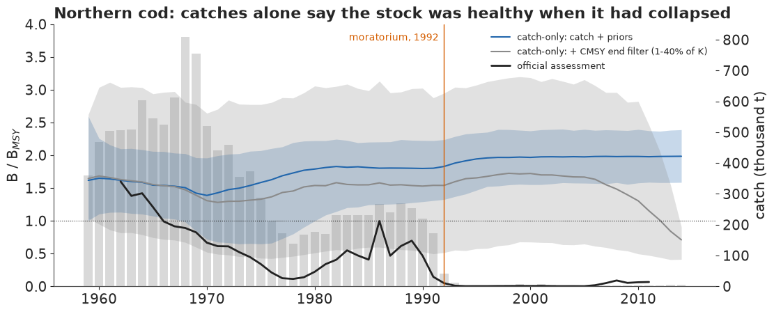
The catch-only posterior misses the collapse completely. In 1992, when the official assessment puts northern cod at about 5% of BMSY, the catch-only model puts it near twice BMSY, and its 2014 range does not reach below about 1.6. CMSY's end filter forces 2014 down to about 0.7, but that is the rule speaking, and it does not reach back to the collapse: 1992 stays at about 1.5, with about a 1-in-20 chance of being below half the healthy level. The wall fights 22 years of near-zero catches during which the dynamics, with a growth rate of about 0.34, regrow any stock; some 200 divergences show the strain. Both histories are negatively correlated with the official one.
Could the model have shown the collapse at all? Its smooth floor and feasibility penalty (at 3% and 2% of $K$) set the lowest state it can represent, about 0.04 of BMSY, above the official 0.003-0.01 of 1993-2005. With both about ten times lower nothing changes: 1992 comes out at about 1.8, and 95% of the draws never go below about 0.5 in any year. The miss is what catches mean. A catch series that rises and falls fits a stock that was fished down (the catch fell because there were no fish) and one that was lightly fished (the catch fell because of a moratorium). Without an index the prior and dynamics choose: the prior paths that survive the catches are big stocks (part C), and falling catches plus a positive growth rate mean recovery. Free et al. (2020, Fisheries Research, "Blood from a stone") tested catch-only methods against full assessments and gave their verdict in the title.
The same blindness on stocks we know
The northern cod result could be a peculiarity of that stock. Refitting three data-rich stocks from part D without their indices tests that:
rows = []
t0 = time.time()
for sid in ("PCODWCVANI", "YELL3LNO", "REDFISHSPP3LN"):
    dco = prep([sid], use_index=False, multi_only=False)
    idc, _ = sample(ss_model(dco, eps=0.03, pen=0.02), dco, RANDOM_SEED)
    bbc, _ = status(idc, dco)
    off = stock_rows(sid).bdivbmsy.to_numpy()
    ok = ~np.isnan(off)
    s = MAIN.index(sid)
    rows.append(dict(stock=NICE[sid], year=int(dco["years"][-1]),
                     catch_only=np.median(bbc[:, -1]), with_index=np.median(BB[:, D["last"][s]]),
                     official=off[ok][-1],
                     corr_catch_only=np.corrcoef(np.log(np.median(bbc, 0)[ok]),
                                                 np.log(off[ok]))[0, 1],
                     divergences=int(idc.sample_stats["diverging"].sum())))
    del idc
TIMES["catch-only refits"] = time.time() - t0
print(pd.DataFrame(rows).set_index("stock").round(2).to_string())
                                  year  catch_only  with_index  official  corr_catch_only  divergences
stock
Pacific cod, W. Vancouver Island  2001        1.76        0.41      0.67            -0.17            5
Yellowtail flounder, Grand Banks  2014        1.70        2.40      1.76             0.86            1
Redfish, Grand Banks              2013        1.78        1.50      1.31             0.61            2
Without its index, every stock ends well above BMSY, at about 1.7 to 1.8 times it. The last-year value is roughly the same whatever happened: catches fell at the end of every one of these records, and the model reads falling catches as regrowth. For Grand Banks yellowtail, which really did recover, the answer is right by luck. For Pacific cod off western Vancouver Island, which was depleted in 2001, it is wrong in the direction that matters.
G · Explaining it to everyone
The statistician's plot
A stock assessment report shows each stock's B/BMSY as a posterior median with a shaded interval. Here it is for the six stocks of the headline, chosen to cover the cod, sole and hake of the question and both agreement and disagreement with the official assessments.
SHOW = ["PCODHS", "PCODWCVANI", "RSOLEHSTR", "YELL3LNO", "SHAKE4VWX", "SPHAKECH"]
fig, axs = plt.subplots(2, 3, figsize=(12, 6.6), sharey=True)
for a, sid in zip(axs.flat, SHOW):
    s = MAIN.index(sid)
    sel = D["st"] == s
    y, b = D["years"][sel], BB[:, sel]
    a.fill_between(y, *np.quantile(b, [0.055, 0.945], axis=0), color=HI, alpha=0.3, lw=0,
                   label="89% interval")
    a.plot(y, np.median(b, 0), color=HI, lw=1.5, label="posterior median")
    g = stock_rows(sid)
    a.plot(g.year, g.bdivbmsy, color=INK, lw=1, label="official")
    a.axhline(1, color=INK, lw=0.7, ls=":")
    a.set_ylim(0, 4.4)
    a.set_title(NICE[sid], loc="left", fontsize=11)
axs[0, 0].legend(fontsize=9, loc="upper right")
axs[0, 0].set_ylabel("B / B$_{MSY}$")
axs[1, 0].set_ylabel("B / B$_{MSY}$")
fig.suptitle("The conventional view: posterior median and 89% interval", x=0.01, ha="left",
             fontsize=13);
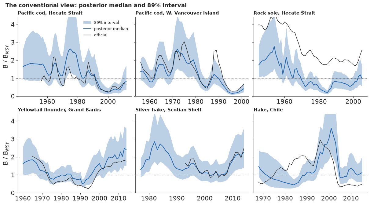
For a trained reader this is the right plot. For anyone else it has three problems. The band reads as a physical object that "grows" where it widens, the error people make with the hurricane "cone of uncertainty" (Ruginski et al. 2016, Spatial Cognition & Computation). The median looks like what happened, although it is smoother than every real history. And the band's edges look like limits.
Forty possible histories
The public version draws 40 posterior paths instead, each a complete history the stock might have had, thin and translucent so that where they crowd the eye sees confidence. Padilla, Ruginski & Creem-Regehr (2017, Cognitive Research) found that ensembles avoid the cone's size misreading but bring a bias of their own: readers over-weight wherever a single line falls. So we use 40 lines at low opacity, highlight none, add no median (Kale, Kay & Hullman 2021, IEEE TVCG, found that a mean mark pulls readers away from the uncertainty), and say on the figure that each line is one possible history. Each title is a count from the 40 paths, the catches sit underneath as grey bars, and the years with an index are shaded: that is where the model "sees" the fish.
PICK = np.random.default_rng(114).choice(BB.shape[0], 40, replace=False)
SHORT = {"PCODHS": "Pacific cod, Hecate Strait", "PCODWCVANI": "Pacific cod, W. Vancouver I.",
         "RSOLEHSTR": "Rock sole, Hecate Strait", "YELL3LNO": "Yellowtail flounder, Grand Banks",
         "SHAKE4VWX": "Silver hake, Scotian Shelf", "SPHAKECH": "Hake, Chile"}


def panel_title(sid, paths, y):
    """A sentence from the 40 paths: the decade in which most fall below half of B_MSY."""
    dec = (y // 10) * 10
    counts = {int(D_): int((paths[:, dec == D_] < 0.5).any(axis=1).sum()) for D_ in np.unique(dec)}
    best = max(counts, key=counts.get)
    if counts[best] >= 10:
        return (f"{SHORT[sid]}\n{counts[best]} of 40 histories fall below half\n"
                f"the healthy level in the {best}s")
    n_any = int((paths < 0.5).any(axis=1).sum())
    return f"{SHORT[sid]}\nonly {n_any} of 40 histories ever fall\nbelow half the healthy level"


DISAGREE = {"RSOLEHSTR": "the official assessment uses\nanother yardstick and index:\n"
                         "see parts D and G",
            "SPHAKECH": "the official assessment\ndisagrees here: see part D"}


def headline_figure():
    fig, axs = plt.subplots(2, 3, figsize=(13, 9.0), layout="none", dpi=80)  # ~40% lighter
    fig.subplots_adjust(left=0.055, right=0.94, top=0.78, bottom=0.05, wspace=0.32, hspace=0.55)
    for j, (a, sid) in enumerate(zip(axs.flat, SHOW)):
        s = MAIN.index(sid)
        sel = D["st"] == s
        y, paths = D["years"][sel], BB[PICK][:, sel]
        g = stock_rows(sid)
        ac = a.twinx()
        ac.bar(g.year, g.catch_t / 1e3, color=LIGHT, width=0.8, zorder=0)
        ac.set_ylim(0, g.catch_t.max() / 1e3 * 2.6)  # top tick well clear of the 0.5 and 1 lines
        ac.set_yticks([0, round(g.catch_t.max() / 1e3)])
        ac.tick_params(labelsize=9, colors=MUTED)
        ac.grid(False)
        if j % 3 == 2:
            ac.set_ylabel("catch, thousand t", fontsize=9.5, color=MUTED, labelpad=4)
        iy = g.year[g.cpue.notna() | g.survey.notna()]
        ac.axvspan(iy.min() - 0.5, iy.max() + 0.5, color="#eef3f8", zorder=-2, lw=0)
        a.set_zorder(ac.get_zorder() + 1)
        a.patch.set_visible(False)
        for p in paths:
            a.plot(y, p, color=HI, alpha=0.18, lw=0.9)
        a.axhline(1, color=INK, lw=1.1)
        a.axhline(0.5, color=LO, lw=1.1, ls="--")
        ok = g.bdivbmsy.notna()
        a.plot(g.year[ok], g.bdivbmsy[ok], color=INK, lw=1.6)
        a.set_ylim(0, 4.4)
        a.set_xlim(y[0] - 1, y[-1] + 1)
        a.tick_params(labelsize=10)
        a.set_title(panel_title(sid, paths, y), loc="left", fontsize=11, color=INK)
        p_last = (BB[:, sel][:, -1] < 1).mean()  # the full posterior, not the 40 lines
        k10 = round(10 * p_last)
        k_txt = ("fewer than 1" if k10 == 0 else "nearly 10" if k10 == 10 else f"about {k10}")
        a.text(0.98, 0.97, f"{y[-1]}: {k_txt} in 10\nbelow the healthy level",
               transform=a.transAxes, ha="right", va="top", fontsize=9.5, color=INK,
               bbox=dict(fc="white", ec="none", alpha=0.85, pad=1.5))
        if sid in DISAGREE:
            a.text(0.98, 0.80, DISAGREE[sid], transform=a.transAxes, ha="right", va="top",
                   fontsize=9, color=MUTED, style="italic",
                   bbox=dict(fc="white", ec="none", alpha=0.85, pad=1.5))
        if j % 3 == 0:
            a.set_ylabel("fish in the sea / healthy level", fontsize=10.5)
        for yv, txt, c in ((1.0, "healthy level", INK), (0.5, "overfished", LO)):
            a.text(0.015, yv + 0.03, txt, transform=a.get_yaxis_transform(), fontsize=9, color=c,
                   va="bottom", bbox=dict(fc="white", ec="none", alpha=0.7, pad=0.8))
    fig.text(0.01, 0.985, "Each blue line is one possible history of the fish in the sea, not a "
             "prediction", fontsize=14.5, weight="bold", color=INK, va="top")
    fig.text(0.01, 0.948, wrap("40 histories per stock that fit the catches (grey bars) and the "
                               "surveys or catch rates (shaded years). Where the lines bunch "
                               "the model is sure, which does not make it right; where they "
                               "spread it is not. Black line: the official assessment. Healthy "
                               "level: the stock size that gives the most catch forever "
                               "($B_{MSY}$). Above 2 a stock is bigger than it would be "
                               "unfished, as in a run of good years; lines above 4.4 are cut "
                               "off.", 150),
             fontsize=11, color=MUTED, va="top")
    return fig


fig_top = headline_figure()
HEADLINE.update(fig_top)  # the copy at the top of the notebook
plt.close(fig_top)
headline_figure()
for sid in SHOW:
    sel = D["st"] == MAIN.index(sid)
    print(panel_title(sid, BB[PICK][:, sel], D["years"][sel]).replace("\n", " "),
          f"| last year {int((BB[PICK][:, sel][:, -1] < 1).sum())} of 40 below 1, full posterior "
          f"{(BB[:, sel][:, -1] < 1).mean():.2f} | lines above 4.4: "
          f"{(BB[PICK][:, sel] > 4.4).any(axis=1).sum()} of 40")
Pacific cod, Hecate Strait 40 of 40 histories fall below half the healthy level in the 2000s | last year 25 of 40 below 1, full posterior 0.68 | lines above 4.4: 10 of 40
Pacific cod, W. Vancouver I. 40 of 40 histories fall below half the healthy level in the 1990s | last year 40 of 40 below 1, full posterior 0.99 | lines above 4.4: 2 of 40
Rock sole, Hecate Strait 40 of 40 histories fall below half the healthy level in the 1980s | last year 14 of 40 below 1, full posterior 0.52 | lines above 4.4: 11 of 40
Yellowtail flounder, Grand Banks 19 of 40 histories fall below half the healthy level in the 1990s | last year 0 of 40 below 1, full posterior 0.00 | lines above 4.4: 1 of 40
Silver hake, Scotian Shelf only 1 of 40 histories ever fall below half the healthy level | last year 0 of 40 below 1, full posterior 0.01 | lines above 4.4: 4 of 40
Hake, Chile 30 of 40 histories fall below half the healthy level in the 1980s | last year 15 of 40 below 1, full posterior 0.38 | lines above 4.4: 14 of 40
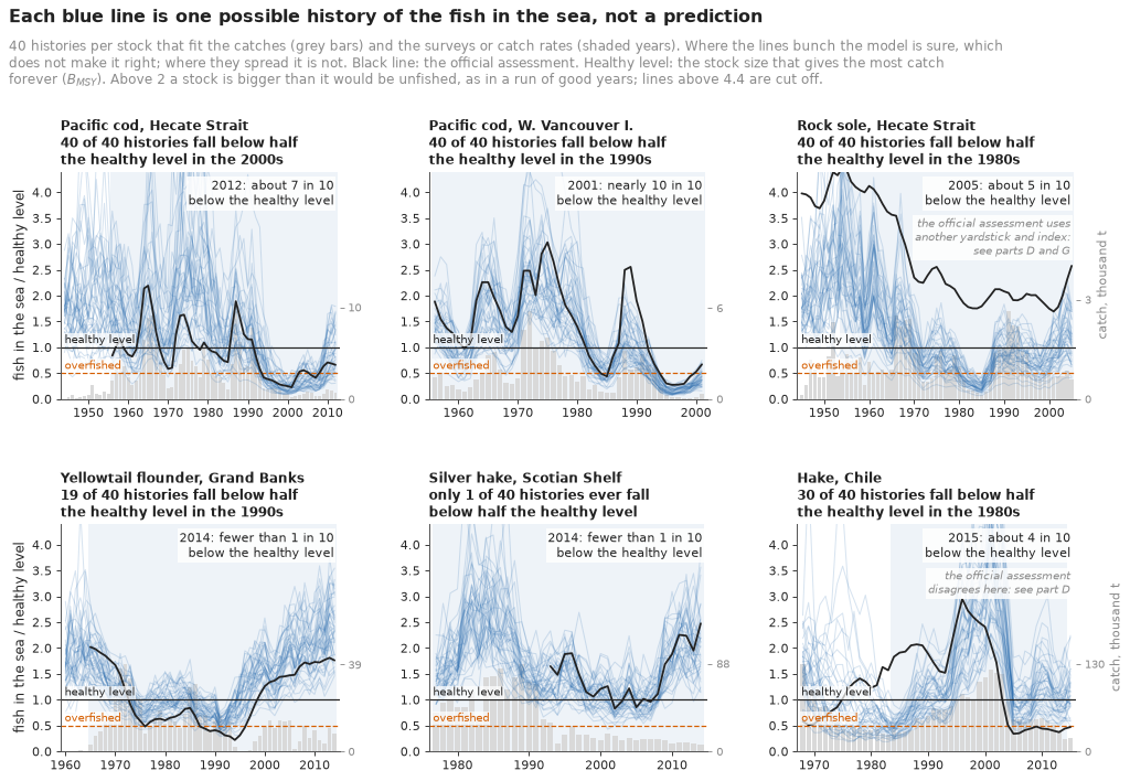
Pacific cod in both areas and Hecate Strait rock sole fall below half the healthy level in every one of the 40 histories, the cod around 2000 and the sole in the 1980s. Grand Banks yellowtail dips in nearly half of them in the 1990s; Scotian Shelf silver hake almost never does. Two panels carry a note because the model and the official assessment disagree. For Hecate Strait rock sole the official line sits at about four times BMSY before 1965 and between 1.7 and 2.6 since about 1970, for the two reasons of part D, so "40 of 40" is our model's verdict alone: a tight bunch of lines says that the model is sure, not that it is right. For Chilean hake about 30 of 40 histories fall below half in the 1980s while the official line sits above it.
Where the record starts before the index (Hecate Strait cod and rock sole, Grand Banks yellowtail, Chilean hake), the lines fan out before it and draw together under it, though a noisy index still lets them spread. Values above 2 mean a stock bigger than it would be unfished, which the process noise allows in a run of good years. Each panel's box gives the last-year chance from the full posterior, rounded to tenths as in the fish rows; the 40 lines are a random sample.
Fish rows: how often is each stock below the line?
The headline shows six stocks over time; "is it below the healthy level now?" needs all 18 at
once, and 18 overlapping Kobe clouds are unreadable. So each stock gets a row of ten fish, an
icon array (Galesic, Garcia-Retamero & Gigerenzer 2009, Health Psychology): in about how
many of ten plausible worlds was the stock below the healthy level in its last year? Solid
vermilion fish are below half of it ("overfished"), hatched ones below it but above half, blue
ones above. public.py draws people, not fish, so the fish glyph is a local helper.
def fish(ax, x, y, s, fc, ec, hatch=None):  # local: the shared module draws people, not fish
    ax.add_patch(Ellipse((x + 0.4 * s, y + 0.5 * s), 0.64 * s, 0.4 * s, fc=fc, ec=ec, hatch=hatch,
                         lw=0.7))
    ax.add_patch(Polygon([(x + 0.68 * s, y + 0.5 * s), (x + 0.94 * s, y + 0.74 * s),
                          (x + 0.94 * s, y + 0.26 * s)], closed=True, fc=fc, ec=ec, hatch=hatch,
                         lw=0.7))


def fish_rows(ax, names, p_half, p_below, n=10):
    """One row of n fish per stock: solid LO below half B_MSY, hatched below B_MSY, HI above."""
    for i, (nm, ph, pb) in enumerate(zip(names, p_half, p_below)):
        y = len(names) - 1 - i
        k_half, k_below = int(round(n * ph)), int(round(n * pb))
        for j in range(n):
            if j < k_half:
                fish(ax, j, y, 0.95, LO, LO)
            elif j < k_below:
                fish(ax, j, y, 0.95, pub._shade(LO, "white", 0.75), LO, "/////")
            else:
                fish(ax, j, y, 0.95, pub._shade(HI, "white", 0.55), HI)
        ax.text(-0.3, y + 0.48, nm, ha="right", va="center", fontsize=10.5, color=INK)
        ax.text(n + 0.2, y + 0.48, f"{k_below} of {n}", ha="left", va="center", fontsize=10.5,
                color=LO if k_below > n / 2 else INK, weight="bold" if k_below > n / 2 else None)
    ax.set_xlim(-0.2, n + 1.4)
    ax.set_ylim(-3.9, len(names) + 0.1)
    ax.set_aspect("equal")
    ax.axis("off")
    for y0, fc, ec, h, txt in ((-1.2, LO, LO, None, "below half the healthy level (overfished)"),
                               (-2.0, pub._shade(LO, "white", 0.75), LO, "/////",
                                "below the healthy level, above half"),
                               (-2.8, pub._shade(HI, "white", 0.55), HI, None,
                                "above the healthy level")):
        fish(ax, 0, y0, 0.8, fc, ec, h)
        ax.text(0.9, y0 + 0.4, txt, fontsize=10, va="center", color=INK)


order = KOBE.index
fig, ax = plt.subplots(figsize=(10, 8.4))
DAG = {nm: ("\u2020\u2020" if v < 0.5 else "\u2020") for nm, v in AGREE.official.items() if v < 1}
fish_rows(ax, [f"{DAG.get(nm, '')} {nm} ({int(KOBE.loc[nm, 'year'])})".strip() for nm in order],
          KOBE.loc[order, "P(B<Bmsy/2)"], KOBE.loc[order, "P(B<Bmsy)"])
other_year = [f"{nm}, {int(AGREE.loc[nm, 'last'])}" for nm in DAG
              if AGREE.loc[nm, "last"] != KOBE.loc[nm, "year"]]
ax.text(-0.2, -3.5, wrap("\u2020 the official assessment put the stock below the healthy level in "
                         "its last assessed year; \u2020\u2020 below half of it (overfished). "
                         "That year is the same as ours except for " + "; ".join(other_year) + ".",
                         72),
        fontsize=9.5, color=MUTED, va="top", ha="left")
print("official marks:", DAG, "| other years:", other_year)
n_rows = int((np.round(10 * KOBE["P(B<Bmsy)"]) > 5).sum())  # the rows drawn, not the raw P
ax.set_title(wrap(f"In the last year of its data, about how many of 10 plausible worlds put each "
                  f"stock below the healthy level? Most do for {n_rows} of the 18 stocks", 80),
             loc="left", fontsize=12.5)
print(f"rows with more than 5 of 10 below: {n_rows}; stocks with P(B<Bmsy) > 0.5: "
      f"{int((KOBE['P(B<Bmsy)'] > 0.5).sum())}");
official marks: {'Pacific cod, W. Vancouver Island': '†', 'Snapper, New Zealand (SNA 7)': '†', 'Pacific cod, Hecate Strait': '†', 'Ling, SE Australia': '†', 'Witch flounder, Gulf of St Lawrence': '††', 'Yellowtail flounder, Georges Bank': '††', 'Hake, Chile': '††'} | other years: ['Yellowtail flounder, Georges Bank, 2007']
rows with more than 5 of 10 below: 3; stocks with P(B<Bmsy) > 0.5: 4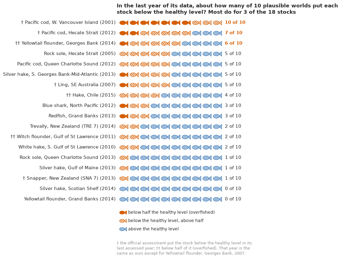
The rows read in a second: Pacific cod off western Vancouver Island at the top with ten of ten, Hecate Strait cod and Georges Bank yellowtail at seven and six, a middle group at four or five that the data cannot call, and a long tail almost certainly above the line. Rounding to tenths costs something at the edge: rock sole (0.52) and Queen Charlotte Sound cod (0.50) both show five of ten, so the rows show three stocks below the line in most worlds where part E counted four. The daggers carry part D's warning onto the figure: witch flounder and snapper look healthy here although their official assessments put them far below the line, and Georges Bank yellowtail is officially overfished, with a survey that ended at a few percent of its 2000s level. Almost all of these stocks were being fished lightly by their last year, which the rows do not show.
Catch against what the stock can give
The savings account has a direct picture: the yearly catch against the withdrawal the account can sustain. MSY is uncertain, so it is a gradient band, darker where more plausible, rather than a line with error bars, which readers take as hard limits (Correll & Gleicher 2014, IEEE TVCG). Catch bars above the band's middle are vermilion: eating the capital.
def msy_band(ax, sid):
    s = MAIN.index(sid)
    sel = D["st"] == s
    yrs = D["years"][sel]
    catch = D["C"][sel] * D["cmax"][s] / 1e3
    msy = np.exp(np.log(DRAW["r"][:, s]) + DRAW["log_K"][:, s]) / 4 * D["cmax"][s] / 1e3
    top = max(catch.max(), np.quantile(msy, 0.99)) * 1.15
    grid = np.linspace(0, top, 300)
    dens = np.histogram(msy, bins=np.r_[grid, grid[-1] + grid[1] - grid[0]])[0].astype(float)
    dens = np.convolve(dens, np.exp(-0.5 * (np.arange(-12, 13) / 4) ** 2), mode="same")
    img = np.zeros((len(grid), 1, 4))
    img[..., :3] = to_rgb(HI)
    img[:, 0, 3] = 0.55 * (dens / dens.max()) ** 0.8
    ax.imshow(img, extent=(yrs[0] - 0.5, yrs[-1] + 0.5, 0, top), aspect="auto", origin="lower",
              interpolation="bilinear", zorder=0)
    over = catch > np.median(msy)
    ax.bar(yrs, catch, color=np.where(over, LO, MUTED), width=0.75, zorder=2)
    ax.set_xlim(yrs[0] - 0.5, yrs[-1] + 0.5)
    ax.set_ylim(0, top)
    ax.set_ylabel("thousand tonnes a year")
    ax.text(yrs[-1], np.quantile(msy, 0.75), "what the stock can\ngive forever (MSY)", color=HI,
            fontsize=10, va="bottom", ha="right", zorder=3,
            bbox=dict(fc="white", ec="none", alpha=0.75, pad=1.5))
    ax.set_title(wrap(f"{NICE[sid]}: the catch took more than the stock could replace in "
                      f"{int(over.sum())} of {len(yrs)} years", 52), loc="left", fontsize=12)
    q = np.quantile(msy, [0.055, 0.5, 0.945])
    print(f"{NICE[sid]}: MSY {q[1] * 1e3:,.0f} t (89% {q[0] * 1e3:,.0f}-{q[2] * 1e3:,.0f}, a "
          f"factor of {q[2] / q[0]:.1f}); catch above the median MSY in {int(over.sum())} of "
          f"{len(yrs)} years: {', '.join(map(str, yrs[over]))}")


fig, axs = plt.subplots(1, 2, figsize=(12.5, 4.4))
for a, sid in zip(axs, ("PCODHS", "YELL3LNO")):
    msy_band(a, sid)
Pacific cod, Hecate Strait: MSY 2,735 t (89% 1,271-5,732, a factor of 4.5); catch above the median MSY in 25 of 69 years: 1957, 1958, 1959, 1963, 1964, 1965, 1966, 1967, 1968, 1972, 1973, 1974, 1975, 1976, 1977, 1979, 1980, 1986, 1987, 1988, 1989, 1990, 1991, 1992, 1993
Yellowtail flounder, Grand Banks: MSY 17,701 t (89% 9,134-34,142, a factor of 3.7); catch above the median MSY in 9 of 55 years: 1970, 1971, 1972, 1973, 1974, 1975, 1979, 1985, 1986
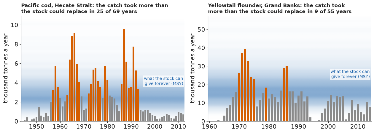
Pacific cod in Hecate Strait took more than it could sustain again and again: 1957-59, 1963-68, most of the 1970s, and 1986-1993, and the headline's histories dive after the last run. Grand Banks yellowtail did so in 1970-1975, 1979 and 1985-86, before its fishery all but closed in the mid-1990s. The band shows a real limit of the method: MSY is a range spanning a factor of about four here, so a catch inside the band is not "safe" or "unsafe" but uncertain.
What the data taught: before and after
The last figure answers the question every Bayesian result invites, "how much of this is the prior?", for the growth rate: grey strips for what biology said before the data, blue for after. Northern cod's catch-only fit is the bottom row.
def before_after(ax, rows, xlim=(0.02, 1.5)):  # local: paired gradient strips, log10 r axis
    lx = np.log10(xlim)
    grid = np.linspace(*lx, 301)
    for i, (nm, pr, po) in enumerate(rows):
        y = len(rows) - 1 - i
        for v, c, dy in ((pr, MUTED, 0.2), (po, HI, -0.2)):
            dens = np.histogram(np.log10(v), bins=grid)[0].astype(float)
            dens = np.convolve(dens, np.exp(-0.5 * (np.arange(-15, 16) / 5) ** 2), mode="same")
            img = np.zeros((1, len(dens), 4))
            img[..., :3] = to_rgb(c)
            img[0, :, 3] = (dens / dens.max()) ** 0.8
            ax.imshow(img, extent=(lx[0], lx[1], y + dy - 0.17, y + dy + 0.17), aspect="auto",
                      interpolation="bilinear", origin="lower", zorder=2)
    ax.set_xlim(*lx)
    ax.set_ylim(-0.6, len(rows) - 0.3)
    ax.set_yticks(range(len(rows)), [nm for nm, _, _ in rows][::-1], fontsize=10)
    ax.tick_params(axis="y", length=0)
    tk = [0.05, 0.1, 0.2, 0.5, 1]
    ax.set_xticks(np.log10(tk), [str(t) for t in tk])
    ax.set_xlabel("growth rate r (per year; log scale)")


ba = [(NICE[sid], np.exp(LOGR_PRIOR[sid]), DRAW["r"][:, MAIN.index(sid)]) for sid in MAIN]
ba.append((NICE["COD2J3KL"] + ", catch only", np.exp(pr_rng.normal(DC["m_r"][0], DC["s_r"][0],
                                                                    n_pr)), R_COD))
fig, ax = plt.subplots(figsize=(10, 8.6))
before_after(ax, ba)
ax.text(1.0, 1.0, "grey: before the data (biology)   blue: after", transform=ax.transAxes,
        ha="right", va="bottom", fontsize=10, color=MUTED)
ax.set_title(wrap("How fast each stock can grow: the data narrowed the range for most stocks, "
                  "moved the hakes, and barely changed it for northern cod's catches alone", 80),
             loc="left", fontsize=12.5, pad=20);
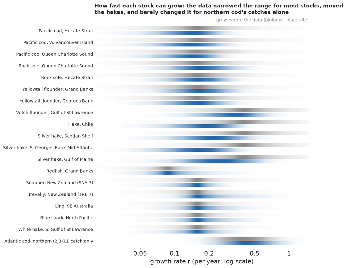
The strips repeat the contraction table in a form that needs no table: the blue strip is a little narrower than the grey for most stocks, clearly shifted for the hakes, and barely changed for the catch-only cod (contraction about 7%): the catches alone carry a little information, by ruling out small, slow stocks that could not have survived them, but not much.
One history at a time
For sharing, the same idea can move. Each frame of the animation is one posterior history of Pacific cod in Hecate Strait, drawn boldly over the faint earlier frames, so the ensemble builds up as the reader watches. This is a hypothetical outcome plot (Hullman, Resnick & Adar 2015, PLOS ONE; Kale, Nguyen, Kay & Hullman 2019, IEEE TVCG): the uncertainty is seen as variation between frames. At 0.7 s a frame it stays well below the three flashes a second that accessibility guidance allows.
NB_STEM = "E114_is_this_fish_overfished"
GIF = f"{NB_STEM}_histories.gif"  # written next to the notebook: the site copies {stem}*.gif
NF = 40
s_k = MAIN.index("PCODHS")
sel_k = D["st"] == s_k
YK = D["years"][sel_k]
PK = BB[PICK][:, sel_k]
gk = stock_rows("PCODHS")
fig_g = plt.figure(figsize=(8, 5.2), dpi=72, layout="none")
ax_g = fig_g.add_axes([0.09, 0.1, 0.84, 0.68])
ax_c = ax_g.twinx()


def history_frame(k):
    ax_g.clear()
    ax_c.clear()
    ax_c.bar(gk.year, gk.catch_t / 1e3, color=LIGHT, width=0.8, zorder=0)
    ax_c.set_ylim(0, gk.catch_t.max() / 1e3 * 2.6)  # the 10 t tick sits well above the 0.5 line
    ax_c.set_yticks([0, 10])
    ax_c.yaxis.tick_right()
    ax_c.yaxis.set_label_position("right")
    ax_c.set_ylabel("catch (thousand t)", color=MUTED)
    ax_c.tick_params(colors=MUTED)
    ax_c.grid(False)
    ax_g.set_zorder(ax_c.get_zorder() + 1)
    ax_g.patch.set_visible(False)
    for j in range(k):
        ax_g.plot(YK, PK[j], color=HI, alpha=0.15, lw=0.9)
    ax_g.plot(YK, PK[k], color=HI, lw=2.2)
    ax_g.axhline(1, color=INK, lw=1.1)
    ax_g.axhline(0.5, color=LO, lw=1.1, ls="--")
    ax_g.text(1945, 1.03, "healthy level", fontsize=10.5, color=INK, va="bottom")
    ax_g.text(1945, 0.53, "overfished", fontsize=10.5, color=LO, va="bottom")
    i_min = int(np.argmin(PK[k]))
    ax_g.plot(YK[i_min], PK[k, i_min], "o", color=HI, ms=7)
    ax_g.set_xlim(YK[0] - 1, YK[-1] + 1)
    ax_g.set_ylim(0, 4.4)
    ax_g.set_ylabel("fish in the sea / healthy level")
    fig_g.texts.clear()
    fig_g.text(0.03, 0.97, f"Pacific cod, Hecate Strait: possible history {k + 1} of {NF}",
               fontsize=14, color=INK, va="top", weight="bold")
    fig_g.text(0.03, 0.905, f"this history's lowest point (dot): {PK[k, i_min]:.2f} of the healthy "
               f"level, in {YK[i_min]}", fontsize=12, color=MUTED, va="top")


t0 = time.time()
frames = pub.save_gif(fig_g, history_frame, NF, GIF, ms=700)
plt.close(fig_g)
TIMES["GIF"] = time.time() - t0
LOWS = YK[np.argmin(PK, axis=1)]
print(f"lowest year of the 40 histories: {np.quantile(LOWS, 0.1):.0f}-{np.quantile(LOWS, 0.9):.0f} "
      f"(middle 80%); {int((PK < 0.5).any(axis=1).sum())} of {NF} fall below half; above 2 before "
      f"1960 in {int((PK[:, YK < 1960] > 2).any(axis=1).sum())}; above 4.4 at some point in "
      f"{int((PK > 4.4).any(axis=1).sum())}")
fig_cs = pub.gif_contact_sheet(frames, title=f"Six of the {NF} possible histories in the "
                                "animation")
fig_cs.set_dpi(80);
wrote E114_is_this_fish_overfished_histories.gif: 40 frames, 576x374 px, 1.0 MB
lowest year of the 40 histories: 1999-2002 (middle 80%); 40 of 40 fall below half; above 2 before 1960 in 33; above 4.4 at some point in 10
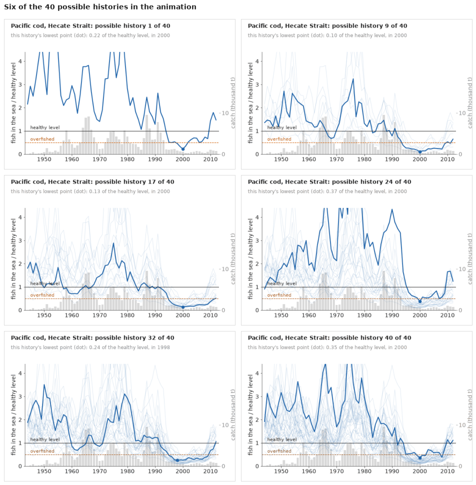
The animation is saved as E114_is_this_fish_overfished_histories.gif, small enough for a message or a slide; the six frames above are its static companion, with the alt text below for screen readers.
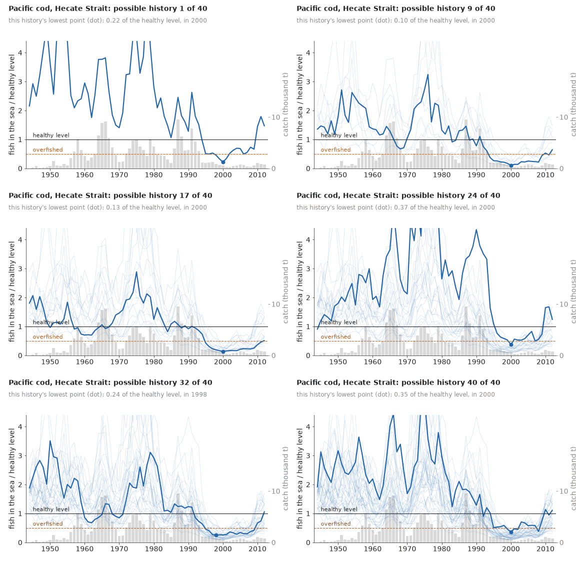
Most histories share that shape: the story of the stock is clear, its exact path is not. Around 2000 the frames barely change; before the index starts, each new frame puts the stock somewhere else.
What the public version gains, and what it costs
The ensemble keeps what the interval plot showed and adds what it lacked: each line is a story a reader can follow, the dives are counted rather than inferred from a band, and no smooth median pretends to be the history. It costs precision (no one can read an 89% interval off 40 lines), and a reader who fixes on the lowest line overstates the risk, which the counted titles are there to correct. It is only as good as the model behind it: for witch flounder, snapper, rock sole, Chilean hake and Georges Bank yellowtail, two reasonable analyses disagree.
TIMES["total"] = time.time() - T_START
print({k: round(v) for k, v in TIMES.items()})
{'toy': 8, 'non-centred': 44, 'centred': 3, 'yellowtail alone': 5, '18 stocks, per-stock noise': 53, '18 stocks': 48, 'yellowtail sensitivity': 13, 'northern cod': 7, 'catch-only refits': 8, 'GIF': 6, 'total': 209}Summary
- A one-way trip cannot separate growth from size. On a simulated stock fished steadily down, $\log r$ and $\log K$ sat on a ridge (correlation $-0.99$, $r$ anywhere in 0.1-1.1, 160 divergences); a recovery after a catch cut narrowed $r$ to 0.33-0.49 around the truth.
- Centred free states beat non-centring here. For Pacific cod the non-centred
scangave r_hat 1.6 and ESS 7; free states sampled in seconds with r_hat about 1.07, the remaining divergences at large process noise. - Sharing noise and biology across 18 stocks. Per-stock process noise gave 114 divergences in 1,000 draws; one shared sd (about 0.24) gave about ten in 4,000 and r_hat at most about 1.02, at the cost of ignoring real differences in noise. Growth rates stay mostly prior; the data moved the hakes from 0.4 to about 0.2.
- Against 14 official assessments the shapes agree well for 7, and the last-year status for 8. Five of the six misses are our model being more optimistic, and none of the three officially overfished stocks (witch flounder, Georges Bank yellowtail, Chilean hake) is overfished in our model. Georges Bank yellowtail's 2014 answer runs from 1.7 to 0.24 times BMSY as the assumed process sd goes from 0.1 to 0.4.
- Below the healthy level, and still fished hard? In the last year of their data (2001-2015) about 6 of the 18 stocks (89% range 3-9) were below BMSY, and at least 4 very likely (94%) were, though we cannot say which; only ling was more likely than not fished above FMSY. Low confidence: a simple model whose $r$ is mostly prior and which, if anything, undercounts.
- Catches alone mislead. Catch-only northern cod came out at about twice BMSY in 1992, against an official 5%, with or without a ten-times-lower floor; CMSY's end filter pulled 2014 down by construction but left 1992 at about 1.5. Three data-rich stocks refitted without their index all ended at 1.7-1.8.
- Ensembles count the dives instead of implying them. 40 possible histories per stock, with counted titles ("40 of 40 fall below half the healthy level in the 1980s"), replace a median and band; fish rows, an MSY gradient band, prior-posterior strips and a HOP GIF support them. The cost: no interval can be read off the lines, a reader who fixes on the lowest line overstates the risk, and tightly bunched lines show the model's certainty, not that it is right (rock sole).
Try it yourself
- Pella-Tomlinson. Replace the logistic surplus with $\frac{r}{m-1} P (1 - P^{m-1})$ and a shared shape $m \sim \mathrm{LogNormal}(\log 2, 0.3)$, so that BMSY need not be half of $K$. Does the agreement with the official levels improve for Hecate Strait rock sole?
- Hyperstability. Commercial catch rates can hold up while a stock shrinks, as they did for northern cod. Write the index as $I \propto B^{\beta}$ with $\beta \sim \mathrm{LogNormal}(0, 0.3)$ for catch-rate series and $\beta = 1$ for surveys, and see which stocks' $\beta$ moves below 1.
- The small pelagics. Add South African anchovy and sardine (in the data file as index stocks) to the main fit, then give them their own process noise. Do the divergences come back, and does a model with a year effect shared by the two (one ocean, two species) fit better?