Most regressions with many candidate predictors carry a belief that is not written down in a Normal prior: most of these variables do nothing, a few do a lot. A Normal prior cannot say that - it shrinks every coefficient by the same factor. Sparse priors can: they pull noise coefficients hard towards zero while leaving large signals almost alone.
This notebook is the dedicated treatment of those priors. E19 already uses a regularised horseshoe inside neighbourhood selection for a graph (and shows how the horseshoe breaks when it is placed on a precision matrix); here we look at the prior itself: what it assumes, how to set its one important knob, why the plain version makes NUTS diverge, how it compares with the discrete spike-and-slab that many people have in mind when they say "variable selection", and how to go from a posterior to an actual choice of variables.
Two datasets. Prostate (8 predictors) is small enough to enumerate every one of the 256 submodels exactly, so we can check what NUTS gets right. Diabetes (64 predictors, 120 training patients, 322 held out) is where the shrinkage is needed, the geometry gets hard, and the predictors are strongly correlated.
import itertools
import logging
import time

import arviz as az
import matplotlib.pyplot as plt
import numpy as np
import pandas as pd
import pymc as pm
import pytensor.tensor as pt
from pymc_extras.marginal import marginalize
from scipy import stats
from scipy.special import betaln, logsumexp

from pymc_challenges import data

RANDOM_SEED = 42
rng = np.random.default_rng(RANDOM_SEED)
az.style.use("arviz-variat")
logging.getLogger("pymc").setLevel(logging.WARNING)  # many small fits: no banner for each
BLUE, ORANGE, AQUA, GREY, PURPLE = "#2a78d6", "#eb6834", "#1baf7a", "#8a8a86", "#8e5bd0"
print(f"PyMC {pm.__version__}, ArviZ {az.__version__}")


def fit(model, label, target_accept=0.8, **kw):
    """Sample with nutpie and print the diagnostics we care about in one line."""
    t0 = time.time()
    with model:
        idata = pm.sample(target_accept=target_accept, random_seed=RANDOM_SEED, progressbar=False, **kw)
    names = [v for v in ["beta", "tau", "sigma"] if v in idata.posterior]
    s = az.summary(idata, var_names=names)
    div = int(idata.sample_stats["diverging"].sum())
    print(f"{label:<38} {time.time() - t0:5.1f} s  divergences {div:4d}  max r_hat {s['r_hat'].max():.3f}  "
          f"min ess_bulk {s['ess_bulk'].min():5.0f}")
    return idata


def draws(idata, var):
    """Posterior draws as a (sample, ...) NumPy array."""
    return idata.posterior[var].stack(sample=("chain", "draw")).transpose("sample", ...).to_numpy()
PyMC 6.3.2, ArviZ 1.3.0
1 · Prostate: eight predictors, 67 training men
The response is log prostate-specific antigen (lpsa), measured before surgery in 97 men;
the predictors are log cancer volume, log prostate weight, age, log benign prostatic
hyperplasia amount, seminal vesicle invasion (0/1), log capsular penetration, Gleason score
and the percentage of Gleason scores 4 or 5. The data come with a fixed split into 67
training and 30 test men, which we keep. Everything is standardised with the training means
and sds, so every coefficient is "sd of log PSA per sd of predictor" and one prior scale fits
all of them.
data.describe("prostate")
pr = data.load("prostate")
PR_NAMES = pr.columns[:8].tolist()
is_train = pr["train"].eq("T").to_numpy()
Xraw, yraw = pr[PR_NAMES].to_numpy(float), pr["lpsa"].to_numpy(float)
x_mu, x_sd = Xraw[is_train].mean(0), Xraw[is_train].std(0)
y_mu, y_sd = yraw[is_train].mean(), yraw[is_train].std()
Xp, yp = (Xraw - x_mu) / x_sd, (yraw - y_mu) / y_sd
Xp_tr, yp_tr, Xp_te, yp_te = Xp[is_train], yp[is_train], Xp[~is_train], yp[~is_train]
n_p, P_p = Xp_tr.shape

b_ols = np.linalg.lstsq(np.c_[np.ones(n_p), Xp_tr], yp_tr, rcond=None)[0][1:]
print(f"{n_p} training men, {len(yp_te)} test men, {P_p} predictors")
pd.DataFrame(np.corrcoef(Xp_tr.T), index=PR_NAMES, columns=PR_NAMES).round(2)
prostate: 97 men: log PSA (lpsa) and 8 clinical predictors (log cancer volume lcavol, log prostate weight lweight, age, lbph, seminal vesicle invasion svi, lcp, gleason, pgg45), plus the book's train/test flag (67 T / 30 F).
  source: Stamey et al. (1989, J. Urology 141:1076), prostate cancer before radical prostatectomy; the benchmark of Hastie, Tibshirani & Friedman, The Elements of Statistical Learning (2009), ch. 3.
  url:    https://hastie.su.domains/ElemStatLearn/datasets/prostate.data
67 training men, 30 test men, 8 predictors
| lcavol | lweight | age | lbph | svi | lcp | gleason | pgg45 | |
|---|---|---|---|---|---|---|---|---|
| lcavol | 1.00 | 0.30 | 0.29 | 0.06 | 0.59 | 0.69 | 0.43 | 0.48 |
| lweight | 0.30 | 1.00 | 0.32 | 0.44 | 0.18 | 0.16 | 0.02 | 0.07 |
| age | 0.29 | 0.32 | 1.00 | 0.29 | 0.13 | 0.17 | 0.37 | 0.28 |
| lbph | 0.06 | 0.44 | 0.29 | 1.00 | -0.14 | -0.09 | 0.03 | -0.03 |
| svi | 0.59 | 0.18 | 0.13 | -0.14 | 1.00 | 0.67 | 0.31 | 0.48 |
| lcp | 0.69 | 0.16 | 0.17 | -0.09 | 0.67 | 1.00 | 0.48 | 0.66 |
| gleason | 0.43 | 0.02 | 0.37 | 0.03 | 0.31 | 0.48 | 1.00 | 0.76 |
| pgg45 | 0.48 | 0.07 | 0.28 | -0.03 | 0.48 | 0.66 | 0.76 | 1.00 |
Moderate correlations: cancer volume goes with capsular penetration (0.69) and seminal vesicle invasion (0.59), and the two Gleason variables with each other (0.76). Nothing pathological - which is why this is the dataset for intuition.
2 · What a shrinkage prior does: the shrinkage factor $\kappa$
Write every prior in the family we care about as a scale mixture of Normals,
$$\beta_j \mid \lambda_j, \tau \sim \text{Normal}(0,\ \tau\lambda_j),$$
with a global scale $\tau$ shared by all coefficients and a local scale $\lambda_j$ for each. For a Normal prior (ridge) $\lambda_j = 1$; for the Laplace (Bayesian lasso) $\lambda_j^2 \sim \text{Exponential}$; for the horseshoe (Carvalho, Polson & Scott 2010) $\lambda_j \sim \text{HalfCauchy}(1)$.
With standardised, roughly uncorrelated predictors the posterior mean of $\beta_j$ given the scales is the least-squares estimate multiplied by $1 - \kappa_j$, where
$$\kappa_j = \frac{1}{1 + n\,\tau^2\lambda_j^2/\sigma^2} \in (0, 1)$$
is the shrinkage factor: $\kappa_j = 0$ leaves the coefficient alone, $\kappa_j = 1$ sets it to zero. The prior on $\lambda_j$ therefore is a prior on how much each coefficient is shrunk. Here is that prior for the three families, at the global scale where $n\tau^2/\sigma^2 = 1$.
S = 200_000
lam = {
    "Normal (ridge)": np.ones(S),
    "Laplace (Bayesian lasso)": np.sqrt(rng.exponential(2.0, S)),     # lambda^2 ~ Exp(mean 2): Laplace(0, 1)
    "horseshoe": np.abs(stats.cauchy.rvs(size=S, random_state=rng)),
}
fig, axes = plt.subplots(1, 3, figsize=(15, 4.2))
for (name, l), col in zip(lam.items(), [GREY, BLUE, ORANGE]):
    b = rng.normal(0, 1, S) * l
    h, e = np.histogram(b, bins=240, range=(-6, 6), density=True)
    axes[0].plot(0.5 * (e[1:] + e[:-1]), h, color=col, label=name)
    axes[1].plot(0.5 * (e[1:] + e[:-1]), h, color=col)
    kappa = 1 / (1 + l**2)
    if name.startswith("Normal"):
        axes[2].axvline(0.5, color=col, lw=2, label=f"{name}: all at 0.5")
    else:
        axes[2].hist(kappa, bins=50, range=(0, 1), density=True, histtype="step", lw=2, color=col, label=name)
axes[0].set(xlim=(-3, 3), xlabel=r"$\beta$ (scale $\tau$ = 1)", ylabel="prior density", title="near zero")
axes[1].set(yscale="log", ylim=(1e-4, 5), xlabel=r"$\beta$", title="tails (log scale)")
axes[2].set(xlabel=r"shrinkage factor $\kappa$", ylabel="prior density", ylim=(0, 4),
            title=r"prior on $\kappa$ when $n\tau^2/\sigma^2 = 1$")
axes[0].legend(fontsize=9)
axes[2].legend(fontsize=9, loc="upper center");
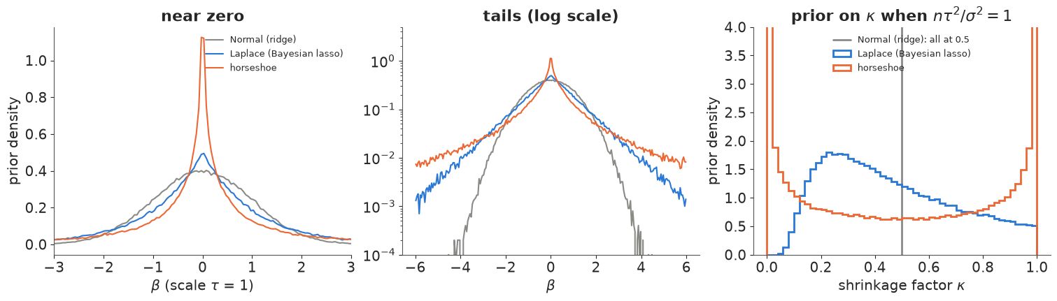
The right panel is the whole argument for the horseshoe. Its $\kappa$ prior is $\text{Beta}(\tfrac12, \tfrac12)$: a U shape with mass piled at both ends, i.e. "each coefficient is either shrunk almost completely or barely at all". The Laplace prior puts its $\kappa$ mass in the middle and has no pole at $\kappa = 0$ - it shrinks large coefficients by a fixed amount (the lasso's well-known bias) and, as we will see, never shrinks small ones all the way. The Normal shrinks every coefficient by the same factor. The left panels say the same thing in terms of $\beta$: the horseshoe has an infinitely tall spike at zero and Cauchy tails.
3 · Three priors on the prostate data
All three models share an intercept, $\sigma \sim \text{HalfNormal}(1)$ and a global scale learned from the data; they differ only in the local scales. All are written non-centred ($\beta_j = z_j\,\tau\lambda_j$ with $z_j \sim \text{Normal}(0, 1)$) except the Laplace, which PyMC samples directly.
def sparse_lm(X, y, prior, names, tau0=1.0, slab_df=4.0, slab_scale=1.0, centred=False, slab=True):
    """Linear regression with standardised predictors and one of several coefficient priors."""
    n, P = X.shape
    with pm.Model(coords={"pred": names}) as model:
        a = pm.Normal("a", 0.0, 1.0)
        sigma = pm.HalfNormal("sigma", 1.0)
        if prior == "ridge":
            tau = pm.HalfNormal("tau", 1.0)
            beta = pm.Deterministic("beta", pm.Normal("z", 0.0, 1.0, dims="pred") * tau, dims="pred")
        elif prior == "lasso":
            tau = pm.HalfNormal("tau", 1.0)
            beta = pm.Laplace("beta", 0.0, tau, dims="pred")
        elif prior == "horseshoe":
            tau = pm.HalfCauchy("tau", tau0)
            lam = pm.HalfCauchy("lam", 1.0, dims="pred")
            if centred:
                beta = pm.Normal("beta", 0.0, tau * lam, dims="pred")
            else:
                beta = pm.Deterministic("beta", pm.Normal("z", 0.0, 1.0, dims="pred") * tau * lam, dims="pred")
        elif prior == "reg_horseshoe":
            # Piironen & Vehtari (2017): tau ~ HalfCauchy(tau0 * sigma), slab c^2 ~ InvGamma(nu/2, nu s^2/2)
            tau = pm.Deterministic("tau", pm.HalfCauchy("tau_raw", 1.0) * tau0 * sigma)
            lam = pm.HalfCauchy("lam", 1.0, dims="pred")
            if slab:
                c2 = pm.InverseGamma("c2", slab_df / 2, slab_df * slab_scale**2 / 2)
                lam_t = pt.sqrt(c2 * lam**2 / (c2 + tau**2 * lam**2))
            else:                                     # the p0-based global scale without the slab
                lam_t = lam
            beta = pm.Deterministic("beta", pm.Normal("z", 0.0, 1.0, dims="pred") * tau * lam_t, dims="pred")
        pm.Normal("y", a + pt.as_tensor(X) @ beta, sigma, observed=y)
    return model


fits_pr = {name: fit(sparse_lm(Xp_tr, yp_tr, name, PR_NAMES), f"prostate, {name}", target_accept=0.99)
           for name in ["ridge", "lasso", "horseshoe"]}
prostate, ridge 1.8 s divergences 0 max r_hat 1.006 min ess_bulk 709
prostate, lasso 0.7 s divergences 0 max r_hat 1.001 min ess_bulk 1964
prostate, horseshoe 1.2 s divergences 20 max r_hat 1.006 min ess_bulk 1031
All three at target_accept=0.99, because the horseshoe needs it and a fair comparison uses
the same settings. The coefficients side by side, with least squares as the unshrunk
reference:
cols = {"ridge": GREY, "lasso": BLUE, "horseshoe": ORANGE}
fig, axes = plt.subplots(1, 2, figsize=(14, 4.6), gridspec_kw={"width_ratios": [1.5, 1]})
ax = axes[0]
for k, (name, idata) in enumerate(fits_pr.items()):
    B = draws(idata, "beta")
    lo, med, hi = np.quantile(B, [0.05, 0.5, 0.95], axis=0)
    yy = np.arange(P_p) + 0.22 * (k - 1)
    ax.hlines(yy, lo, hi, color=cols[name], lw=2)
    ax.plot(med, yy, "o", color=cols[name], label=name)
ax.plot(b_ols, np.arange(P_p), "kx", ms=8, label="least squares")
ax.axvline(0, color=GREY, lw=0.8, ls="--")
ax.set(yticks=range(P_p), xlabel="coefficient (sd of log PSA per sd)", title="posterior median and 90% interval")
ax.set_yticklabels(PR_NAMES)
ax.invert_yaxis()
ax.legend(fontsize=9, loc="lower right")
ax = axes[1]
j = PR_NAMES.index("gleason")
for name in ["ridge", "lasso", "horseshoe"]:
    b = draws(fits_pr[name], "beta")[:, j]
    ax.hist(b, bins=120, range=(-0.5, 0.5), density=True, histtype="step", lw=2, color=cols[name],
            label=f"{name}: P(|beta| < 0.02) = {np.mean(np.abs(b) < 0.02):.2f}")
ax.set(xlabel="coefficient of gleason", yticks=[], title="a null-looking coefficient")
ax.legend(fontsize=9);
tab = pd.DataFrame({"least squares": b_ols} | {name: np.median(draws(i, "beta"), 0) for name, i in fits_pr.items()},
                   index=PR_NAMES)
tab.loc["global scale tau (median)"] = [np.nan] + [np.median(draws(i, "tau")) for i in fits_pr.values()]


def rmse_test(a, B):
    return np.sqrt(np.mean(((a + B @ Xp_te.T).mean(0) - yp_te) ** 2)) * y_sd   # log PSA units


a_ols = yp_tr.mean() - Xp_tr.mean(0) @ b_ols
tab.loc["test RMSE, 30 men"] = [rmse_test(np.array([a_ols]), b_ols[None, :])] + [
    rmse_test(draws(i, "a")[:, None], draws(i, "beta")) for i in fits_pr.values()]
tab.round(3)
| least squares | ridge | lasso | horseshoe | |
|---|---|---|---|---|
| lcavol | 0.593 | 0.507 | 0.529 | 0.550 |
| lweight | 0.242 | 0.239 | 0.228 | 0.217 |
| age | -0.118 | -0.091 | -0.069 | -0.037 |
| lbph | 0.176 | 0.166 | 0.151 | 0.128 |
| svi | 0.256 | 0.234 | 0.215 | 0.173 |
| lcp | -0.239 | -0.137 | -0.109 | -0.051 |
| gleason | -0.017 | 0.009 | 0.011 | 0.004 |
| pgg45 | 0.230 | 0.174 | 0.141 | 0.091 |
| global scale tau (median) | NaN | 0.284 | 0.235 | 0.214 |
| test RMSE, 30 men | 0.722 | 0.705 | 0.692 | 0.677 |
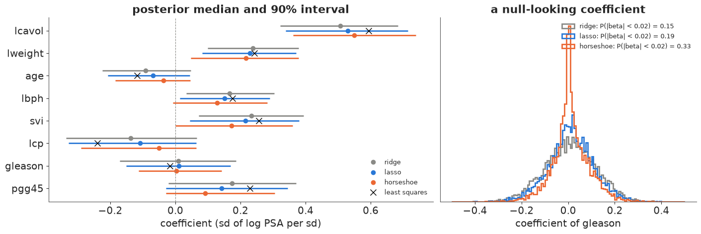
All three agree on the big picture - cancer volume dominates, prostate weight, seminal
vesicle invasion and lbph push log PSA up, Gleason score adds nothing once the rest is
known. On the 30 test men the horseshoe predicts best and least squares worst (RMSE 0.68
against 0.72 log-PSA units), with ridge and lasso in between, but 30 men are too few to make
much of differences that size. Where the priors really differ is in how they shrink:
- Ridge has one scale for everything, so the strongest coefficient pays too:
lcavolloses about 15% (0.59 to 0.51), while the weakpgg45keeps three quarters of its size. - Horseshoe leaves the strong coefficient almost alone (
lcavol0.55) and pulls the weak, uncertain ones much harder:lcpfrom -0.24 to -0.05,agefrom -0.12 to -0.04,pgg45from 0.23 to 0.09. That is the U-shaped $\kappa$ prior at work. - Laplace sits in between on every row except the null
gleason.
One warning sign already: even at target_accept=0.99 the horseshoe has about 20
divergent transitions in 4000 draws (the other two have none). With 8 well-determined
coefficients this is a minor blemish; section 7 shows what it grows into with 64.
Why the Bayesian lasso's posterior is not sparse
The lasso estimate is the posterior mode under a Laplace prior, and the mode of a
Laplace posterior sits exactly at zero for weak coefficients - that is where the lasso's
zeros come from. But the posterior mass at exactly zero is zero, and the mass near
zero is not much larger than under a Normal prior: the Laplace spike at zero is a kink, not
a pole. Any summary that uses the whole posterior (mean, median, interval, prediction)
is therefore not sparse. In the right panel the posterior probability that the Gleason
coefficient is within 0.02 of zero is 0.15 under ridge, 0.19 under the Laplace and 0.33 under
the horseshoe: the horseshoe's pole at zero is what produces real posterior mass there. And
the Laplace's single rate $\tau$ has two jobs at once - shrinking the noise and leaving the
signal alone - which it cannot both do: compared with the horseshoe it pulls lcavol down
further (0.53 against 0.55) while leaving more of the weak pgg45 (0.14 against 0.09).
4 · Spike-and-slab: the prior people have in mind, and what NUTS can do with it
The "real" variable-selection prior has a discrete indicator per coefficient:
$$\gamma_j \sim \text{Bernoulli}(\pi), \qquad \beta_j \mid \gamma_j = 1 \sim \text{Normal}(0, \sigma v), \qquad \beta_j \mid \gamma_j = 0 = 0 \text{ exactly}.$$
NUTS cannot sample the $\gamma_j$ (they are discrete), and it cannot marginalise them either, because with a point mass at zero the likelihood depends on the whole vector $\gamma$ at once: summing it out means summing over all $2^P$ subsets. For $P = 8$ that is 256 models, and with a conjugate prior each has a closed-form marginal likelihood. So for prostate we can compute the exact posterior inclusion probabilities (PIPs) in a few lines of NumPy: $\sigma^2 \sim \text{InvGamma}(1, 1)$, slab variance $v = 1$ (in units of $\sigma$), a flat intercept (handled by centring) and $\pi \sim \text{Beta}(1, 1)$, which puts equal prior mass on each model size.
V_SLAB, A0, B0 = 1.0, 1.0, 1.0
MODELS = np.array(list(itertools.product([0, 1], repeat=P_p)), dtype=bool)
yc = yp_tr - yp_tr.mean()
log_post = np.empty(len(MODELS))
for m, g in enumerate(MODELS):
    Xc = Xp_tr[:, g] - Xp_tr[:, g].mean(0)
    Sig = np.eye(n_p) + V_SLAB * Xc @ Xc.T              # y | gamma, sigma^2 ~ N(0, sigma^2 Sig)
    _, logdet = np.linalg.slogdet(Sig)
    quad = yc @ np.linalg.solve(Sig, yc)
    k = g.sum()
    log_post[m] = (-0.5 * logdet - (A0 + (n_p - 1) / 2) * np.log(B0 + quad / 2)   # sigma^2 integrated out
                   + betaln(1 + k, 1 + P_p - k))                                  # pi integrated out
w_models = np.exp(log_post - logsumexp(log_post))
pip_exact = w_models @ MODELS
for m in np.argsort(-w_models)[:5]:
    print(f"P(model) = {w_models[m]:.3f}: {', '.join(np.array(PR_NAMES)[MODELS[m]])}")
P(model) = 0.140: lcavol, lweight
P(model) = 0.077: lcavol, lweight, svi
P(model) = 0.066: lcavol, lweight, age, lbph, svi, lcp, gleason, pgg45
P(model) = 0.058: lcavol, lweight, lbph, svi
P(model) = 0.043: lcavol, lweight, pgg45
For NUTS we replace the point mass by a narrow Normal "spike", $\beta_j \mid \gamma_j = 0 \sim
\text{Normal}(0, 0.01\,\sigma)$ - the continuous spike-and-slab of George & McCulloch (1993).
Now $\gamma_j$ touches only $\beta_j$, so each indicator can be summed out on its own
(two terms, not $2^P$): the prior of each $\beta_j$ becomes a two-component Normal mixture.
pymc_extras.marginalize does this rewrite for us from the model written with the
Bernoulli, and afterwards the inclusion probability can be computed exactly given each
posterior draw (Rao-Blackwellised) instead of from sampled 0/1 values.
SPIKE = 0.01


def spike_slab_model(X, y, names):
    with pm.Model(coords={"pred": names}) as model:
        a = pm.Normal("a", 0.0, 1.0)
        s2 = pm.InverseGamma("s2", A0, B0)
        sigma = pm.Deterministic("sigma", pt.sqrt(s2))
        pi = pm.Beta("pi", 1.0, 1.0)
        gamma = pm.Bernoulli("gamma", pi, dims="pred")
        beta = pm.Normal("beta", 0.0, sigma * pt.switch(gamma, np.sqrt(V_SLAB), SPIKE), dims="pred")
        pm.Normal("y", a + pt.as_tensor(X) @ beta, sigma, observed=y)
    return marginalize(model, ["gamma"])


def pip_rao_blackwell(idata):
    """P(gamma_j = 1 | beta_j, sigma, pi) for every draw: the average is the PIP."""
    b, s, p = draws(idata, "beta"), draws(idata, "sigma")[:, None], draws(idata, "pi")[:, None]
    l1 = np.log(p) + stats.norm.logpdf(b, 0, s * np.sqrt(V_SLAB))
    l0 = np.log1p(-p) + stats.norm.logpdf(b, 0, s * SPIKE)
    return 1 / (1 + np.exp(l0 - l1))


idata_ss_pr = fit(spike_slab_model(Xp_tr, yp_tr, PR_NAMES), "prostate, spike-and-slab", target_accept=0.95)
pip_draws = pip_rao_blackwell(idata_ss_pr)
pip_chain = pip_draws.reshape(4, -1, P_p).mean(1)
pd.DataFrame({"exact (enumeration)": pip_exact, "NUTS, all chains": pip_draws.mean(0)}
             | {f"chain {c}": pip_chain[c] for c in range(4)}, index=PR_NAMES).round(2)
prostate, spike-and-slab 1.5 s divergences 0 max r_hat 1.148 min ess_bulk 19
| exact (enumeration) | NUTS, all chains | chain 0 | chain 1 | chain 2 | chain 3 | |
|---|---|---|---|---|---|---|
| lcavol | 1.00 | 1.00 | 1.00 | 1.00 | 1.00 | 1.00 |
| lweight | 0.90 | 0.86 | 0.91 | 0.68 | 0.91 | 0.94 |
| age | 0.27 | 0.30 | 0.42 | 0.16 | 0.24 | 0.39 |
| lbph | 0.51 | 0.51 | 0.62 | 0.49 | 0.30 | 0.62 |
| svi | 0.63 | 0.71 | 0.79 | 0.71 | 0.56 | 0.79 |
| lcp | 0.36 | 0.42 | 0.45 | 0.31 | 0.23 | 0.68 |
| gleason | 0.25 | 0.28 | 0.35 | 0.28 | 0.20 | 0.31 |
| pgg45 | 0.43 | 0.56 | 0.68 | 0.49 | 0.37 | 0.71 |
The exact answer first. No single model dominates: the best, lcavol + lweight, has 14% of
the posterior mass, and the full model with all eight predictors is third - the
Beta(1, 1) prior on $\pi$ gives every model size the same prior mass, so the one full model
is a priori as likely as all 70 four-predictor models together. The PIPs are the useful
summary: lcavol certainly in (1.00), lweight very likely (0.90), svi and lbph a coin
flip (0.63, 0.51), the rest between 0.25 and 0.43.
Now NUTS. Zero divergences - but r_hat around 1.15 and a bulk ESS below 20, and the four
chains give visibly different PIPs (pgg45 and lcp differ between chains by 0.3 or more).
The all-chain average lands in the right neighbourhood of the exact values, but it is off by
up to about 0.13 (pgg45) and there is no way to know that without the enumeration. The divergence
counter says nothing is wrong with the geometry; the problem is mixing between modes, and
only r_hat and ESS reveal it.
fig, axes = plt.subplots(1, 2, figsize=(14, 4))
ax = axes[0]
for name, ls in [("pgg45", "-"), ("age", ":")]:
    j = PR_NAMES.index(name)
    run = np.cumsum(pip_draws[:, j].reshape(4, -1), axis=1) / np.arange(1, pip_draws.shape[0] // 4 + 1)
    for c in range(4):
        ax.plot(run[c], lw=1.2, ls=ls, color=[BLUE, ORANGE, AQUA, PURPLE][c], label=f"chain {c}" if ls == "-" else None)
    ax.axhline(pip_exact[j], color="k", lw=1.5, ls=ls, label=f"exact PIP, {name}")
ax.set(xlabel="draw", ylabel="running PIP", ylim=(0, 1), title="running PIP per chain: pgg45 (solid), age (dotted)")
ax.legend(fontsize=8, ncol=3)
ax = axes[1]
ax.hist(draws(idata_ss_pr, "beta")[:, PR_NAMES.index("svi")], bins=150, range=(-0.3, 0.8), color=BLUE)
ax.set(xlabel="beta[svi]", yticks=[], title="a coefficient with PIP near 0.6: spike + slab, bimodal");
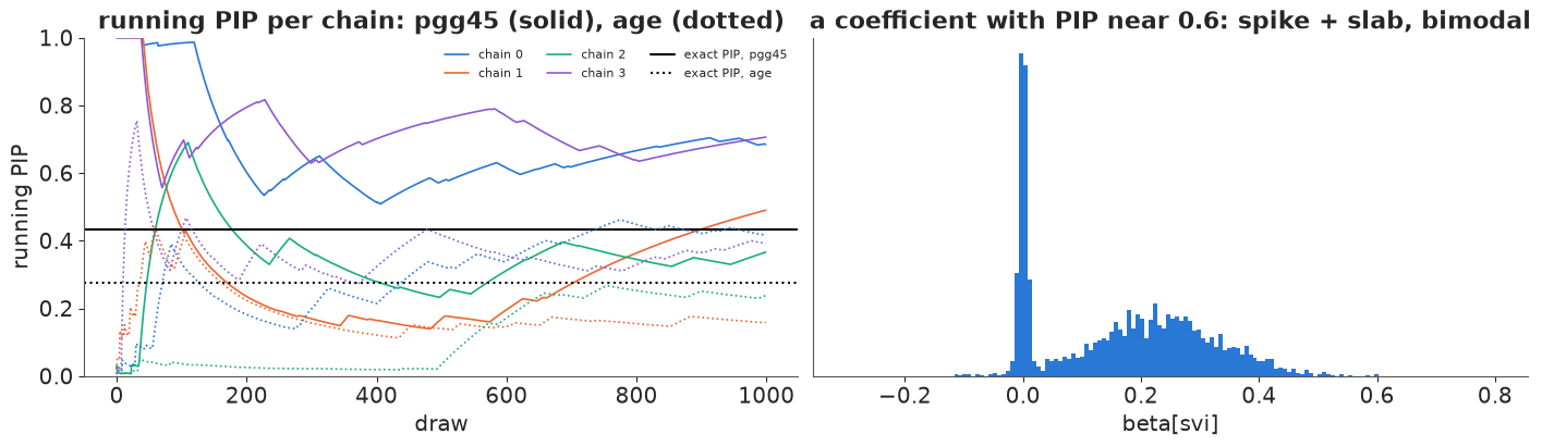
The left panel shows why. A running PIP that moves in long straight stretches is a chain that
sits in the spike (or the slab) for hundreds of draws before switching: each chain makes only
a handful of crossings, so four chains of 1000 draws amount to a few dozen independent
"decisions" per coefficient. The right panel is the posterior of svi: a needle at zero, a
slab around 0.2-0.3, and a thin valley between them that a gradient-based sampler has to
cross. A wider spike makes the valley shallower but then "excluded" no longer means "zero";
a narrower spike makes the valley deeper.
What NUTS can do with a spike-and-slab: sample the continuous relaxation, with the indicators summed out one at a time, and produce Rao-Blackwellised PIPs that are right to within Monte Carlo error that r_hat honestly reports as large. What it cannot do: the point-mass version (a discrete model space), or mix well between "in" and "out". For small $P$ enumerate, as above; for larger $P$ the standard tool is a Gibbs sampler over $\gamma$ with the coefficients integrated out conjugately - not something PyMC's samplers provide.
5 · Diabetes: 64 candidate predictors, 120 patients
The LARS diabetes data (Efron et al. 2004) has ten baseline measurements on 442 patients and a measure of disease progression a year later. Efron et al.'s "quadratic model" adds all 45 pairwise interactions and 9 squares (sex is binary, so no square), for 64 candidate predictors. We build those columns ourselves, fit on a random 120 patients (so $P = 64$ is about half of $n$: least squares is possible but wild) and keep the other 322 as a test set.
data.describe("diabetes")
db = data.load("diabetes")
MAIN = ["age", "sex", "bmi", "bp", "tc", "ldl", "hdl", "tch", "ltg", "glu"]
db.columns = MAIN + ["y"]
perm = rng.permutation(len(db))
tr, te = perm[:120], perm[120:]
Zm = (db[MAIN] - db[MAIN].iloc[tr].mean()) / db[MAIN].iloc[tr].std()
cols64 = {m: Zm[m] for m in MAIN}
cols64 |= {f"{a}:{b}": Zm[a] * Zm[b] for a, b in itertools.combinations(MAIN, 2)}
cols64 |= {f"{m}^2": Zm[m] ** 2 for m in MAIN if m != "sex"}
X64 = pd.DataFrame(cols64)
NAMES = X64.columns.tolist()
X64 = ((X64 - X64.iloc[tr].mean()) / X64.iloc[tr].std()).to_numpy()
yd_mu, yd_sd = db["y"].iloc[tr].mean(), db["y"].iloc[tr].std()
yd = ((db["y"] - yd_mu) / yd_sd).to_numpy()
Xd_tr, yd_tr, Xd_te, yd_te = X64[tr], yd[tr], X64[te], yd[te]
n_d, P_d = Xd_tr.shape
C = np.corrcoef(Xd_tr.T)
iu = np.triu_indices(P_d, 1)
print(f"{n_d} training / {len(te)} test patients, {P_d} predictors")
print(f"pairs with |correlation| > 0.8: {(np.abs(C[iu]) > 0.8).sum()}, > 0.5: {(np.abs(C[iu]) > 0.5).sum()}")
for k in np.argsort(-np.abs(C[iu]))[:5]:
    print(f"  {NAMES[iu[0][k]]:>8} ~ {NAMES[iu[1][k]]:<8} r = {C[iu][k]:+.2f}")
diabetes: 442 diabetes patients: AGE, SEX, BMI, blood pressure BP, six blood serum measurements S1-S6 (S1 total cholesterol, S2 LDL, S3 HDL, S4 total/HDL ratio, S5 log triglycerides, S6 glucose) and Y, a measure of disease progression one year after baseline (raw, unstandardised).
  source: Efron, Hastie, Johnstone & Tibshirani (2004, Ann. Statist. 32:407), 'Least angle regression'; the LARS diabetes data.
  url:    https://web.stanford.edu/~hastie/Papers/LARS/diabetes.data
120 training / 322 test patients, 64 predictors
pairs with |correlation| > 0.8: 16, > 0.5: 104
    tc:ldl ~ ldl^2    r = +0.97
    tc:ldl ~ tc^2     r = +0.97
    age:tc ~ age:ldl  r = +0.95
    tc:tch ~ ldl:tch  r = +0.95
    bmi:tc ~ bmi:ldl  r = +0.95
This is a correlated design by construction: 16 pairs of columns correlate above 0.8 and
over a hundred above 0.5. The worst offenders all involve total cholesterol (tc) and LDL
(ldl), which correlate at 0.94 themselves, so every interaction built from one of them
nearly duplicates the matching interaction built from the other.
6 · Choosing the global scale: a prior guess $p_0$ and the prior on $m_\text{eff}$
With the horseshoe, $\tau$ is the knob that matters. The default $\tau \sim \text{HalfCauchy}(1)$ is meant as "anything goes" on the scale of the data - we will see that it is not. Piironen & Vehtari (2017) derive a better default: if you expect about $p_0$ relevant predictors out of $P$, set
$$\tau_0 = \frac{p_0}{P - p_0}\,\frac{\sigma}{\sqrt n}, \qquad \tau \sim \text{HalfCauchy}(\tau_0).$$
The quantity that justifies this is the effective number of non-zero coefficients $m_\text{eff} = \sum_j (1 - \kappa_j)$, the number of coefficients that escape shrinkage. We should look at its prior before fitting anything - by simulation, because it has no closed form. The guess here: $p_0 = 5$, a deliberately small number (a handful of the ten baseline variables, few or none of the interactions). The regularised horseshoe also has a slab $c$, which we come to in section 7.
def m_eff_prior(n, P, S=20_000, tau0=None, slab=True, sigma_prior=True):
    """Simulate the prior of m_eff = sum_j (1 - kappa_j)."""
    sigma = np.abs(rng.normal(0, 1, S)) if sigma_prior else np.ones(S)
    lam = np.abs(stats.cauchy.rvs(size=(S, P), random_state=rng))
    if tau0 is None:  # plain horseshoe, tau ~ HalfCauchy(1) on the data scale
        tau = np.abs(stats.cauchy.rvs(size=S, random_state=rng))
    else:
        tau = np.abs(stats.cauchy.rvs(size=S, random_state=rng)) * tau0 * sigma
    if slab:
        c2 = stats.invgamma.rvs(2.0, scale=2.0, size=S, random_state=rng)
        lam = np.sqrt(c2[:, None] * lam**2 / (c2[:, None] + tau[:, None] ** 2 * lam**2))
    kappa = 1 / (1 + n * tau[:, None] ** 2 * lam**2 / sigma[:, None] ** 2)
    return (1 - kappa).sum(1)


def tau0_for(p0, P, n):
    return p0 / (P - p0) / np.sqrt(n)


meff = {
    r"horseshoe, $\tau$ ~ HalfCauchy(1)": m_eff_prior(n_d, P_d, slab=False),
    r"regularised, $p_0$ = 5": m_eff_prior(n_d, P_d, tau0=tau0_for(5, P_d, n_d)),
    r"regularised, $p_0$ = 20": m_eff_prior(n_d, P_d, tau0=tau0_for(20, P_d, n_d)),
}
fig, ax = plt.subplots(figsize=(10, 4))
for (name, m), col in zip(meff.items(), [GREY, ORANGE, BLUE]):
    ax.hist(m, bins=64, range=(0, 64), density=True, histtype="step", lw=2, color=col,
            label=f"{name}: median {np.median(m):.1f}, 90% [{np.quantile(m, 0.05):.1f}, {np.quantile(m, 0.95):.1f}]")
ax.set(xlabel=r"$m_\mathrm{eff}$ = effective number of non-zero coefficients (of 64)", yticks=[],
       title=r"prior on $m_\mathrm{eff}$, by simulation")
ax.legend(fontsize=9);
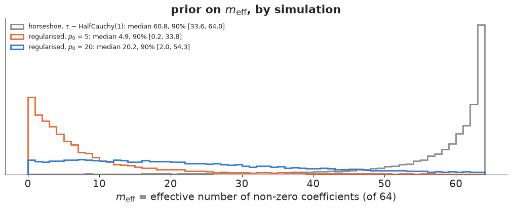
The default horseshoe, with $\tau \sim \text{HalfCauchy}(1)$, puts a prior median of 61 of 64 effective non-zero coefficients: "sparse prior" or not, at this global scale it says that nearly everything matters, which is the opposite of what we believe. The Piironen-Vehtari scale with $p_0 = 5$ puts the median at 5 with a long right tail (90% interval 0.2 to 34), so the data can still ask for many more; $p_0 = 20$ is almost flat over 0-50. $p_0$ is a soft guess, not a hard constraint - and this plot is how to check that the prior you wrote says what you meant.
7 · The failure: a plain horseshoe diverges
First the textbook horseshoe with $\tau \sim \text{HalfCauchy}(1)$, written the obvious
(centred) way, $\beta_j \sim \text{Normal}(0, \tau\lambda_j)$, at the default
target_accept=0.8. Then the changes one at a time: non-centring, a higher
target_accept, the global scale $\tau_0$ from $p_0 = 5$ without a slab, and the full
regularised horseshoe ($p_0$ scale plus slab) at both target_accept values.
TAU0 = tau0_for(5, P_d, n_d)
variants = [
    ("horseshoe, centred, ta 0.8", dict(prior="horseshoe", centred=True), 0.8),
    ("horseshoe, non-centred, ta 0.8", dict(prior="horseshoe"), 0.8),
    ("horseshoe, non-centred, ta 0.99", dict(prior="horseshoe"), 0.99),
    ("p0-scaled horseshoe, no slab, ta 0.99", dict(prior="reg_horseshoe", tau0=TAU0, slab=False), 0.99),
    ("reg. horseshoe, non-centred, ta 0.8", dict(prior="reg_horseshoe", tau0=TAU0), 0.8),
    ("reg. horseshoe, non-centred, ta 0.99", dict(prior="reg_horseshoe", tau0=TAU0), 0.99),
]
fits_d, diag = {}, []
for label, kw, ta in variants:
    idata = fit(sparse_lm(Xd_tr, yd_tr, names=NAMES, **kw), label, target_accept=ta)
    s = az.summary(idata, var_names=["tau"])
    diag.append({"model": label, "divergences": int(idata.sample_stats["diverging"].sum()),
                 "mean tree depth": float(idata.sample_stats["depth"].mean()),
                 "tau r_hat": float(s["r_hat"].iloc[0]), "tau ess_bulk": float(s["ess_bulk"].iloc[0])})
    fits_d[label] = idata
pd.DataFrame(diag).set_index("model").round(2)
horseshoe, centred, ta 0.8 7.0 s divergences 648 max r_hat 1.220 min ess_bulk 14
horseshoe, non-centred, ta 0.8 1.2 s divergences 212 max r_hat 1.010 min ess_bulk 329
horseshoe, non-centred, ta 0.99 1.7 s divergences 29 max r_hat 1.007 min ess_bulk 504
p0-scaled horseshoe, no slab, ta 0.99 1.8 s divergences 18 max r_hat 1.004 min ess_bulk 431
reg. horseshoe, non-centred, ta 0.8 1.2 s divergences 140 max r_hat 1.021 min ess_bulk 379
reg. horseshoe, non-centred, ta 0.99 1.9 s divergences 1 max r_hat 1.003 min ess_bulk 550
| divergences | mean tree depth | tau r_hat | tau ess_bulk | |
|---|---|---|---|---|
| model | ||||
| horseshoe, centred, ta 0.8 | 648 | 9.42 | 1.16 | 18.38 |
| horseshoe, non-centred, ta 0.8 | 212 | 4.90 | 1.01 | 328.73 |
| horseshoe, non-centred, ta 0.99 | 29 | 6.97 | 1.01 | 504.18 |
| p0-scaled horseshoe, no slab, ta 0.99 | 18 | 6.91 | 1.00 | 430.58 |
| reg. horseshoe, non-centred, ta 0.8 | 140 | 4.92 | 1.02 | 378.85 |
| reg. horseshoe, non-centred, ta 0.99 | 1 | 6.31 | 1.00 | 550.49 |
The pattern is typical of horseshoes:
- Centred: several hundred divergences, r_hat 1.2, ESS in the teens, and a mean tree depth above 9, close to nutpie's default cap of 10. Nothing from this fit can be used.
- Non-centred removes the worst of it - r_hat and ESS become respectable - but a couple of
hundred divergences remain at the default
target_accept. target_accept=0.99(smaller steps) brings them down to a few dozen; the $p_0$-based global scale alone to a similar number.- The regularised horseshoe ($p_0$ scale and slab) with
target_accept=0.99has 1 divergence in 4000 draws, and at the default 0.8 it still has over a hundred. No single change is enough; the combination is.
The price is visible in the tree depth: 2-4 times more gradient evaluations per draw than at 0.8. With 120 observations that is seconds.
Where do the divergences sit? In the centred model, the joint posterior of a null coefficient and its scale is Neal's funnel: when $\tau\lambda_j$ is small, $\beta_j$ is squeezed into a tiny interval, and a step size that works in the mouth of the funnel is far too big in its neck.
idc = fits_d["horseshoe, centred, ta 0.8"]
div = idc.sample_stats["diverging"].stack(sample=("chain", "draw")).to_numpy()
B_c = draws(idc, "beta")
scale = draws(idc, "tau")[:, None] * draws(idc, "lam")
j_null = int(np.argmin(np.abs(np.median(B_c, 0))))
j_big = NAMES.index("ltg")
fig, axes = plt.subplots(1, 3, figsize=(15, 4.3))
for ax, j in zip(axes[:2], [j_null, j_big]):
    ax.scatter(np.log(scale[~div, j]), B_c[~div, j], s=3, color=GREY, alpha=0.4, label="draw")
    ax.scatter(np.log(scale[div, j]), B_c[div, j], s=8, color=ORANGE, label="divergent")
    ax.set(xlabel=rf"log($\tau\lambda$) for {NAMES[j]}", ylabel=f"beta[{NAMES[j]}]",
           title=f"centred horseshoe: {NAMES[j]}")
axes[0].legend(fontsize=9, markerscale=3)
ax = axes[2]
for (label, idata), col in zip(fits_d.items(), [GREY, BLUE, AQUA, "k", PURPLE, ORANGE]):
    ax.hist(np.log10(draws(idata, "tau")), bins=60, range=(-5, 0.5), density=True, histtype="step", lw=1.8,
            color=col, label=label)
ax.set(xlabel=r"log$_{10}\tau$", yticks=[], xlim=(-3.5, -0.5), title=r"posterior of the global scale $\tau$")
ax.legend(fontsize=7, loc="upper left");
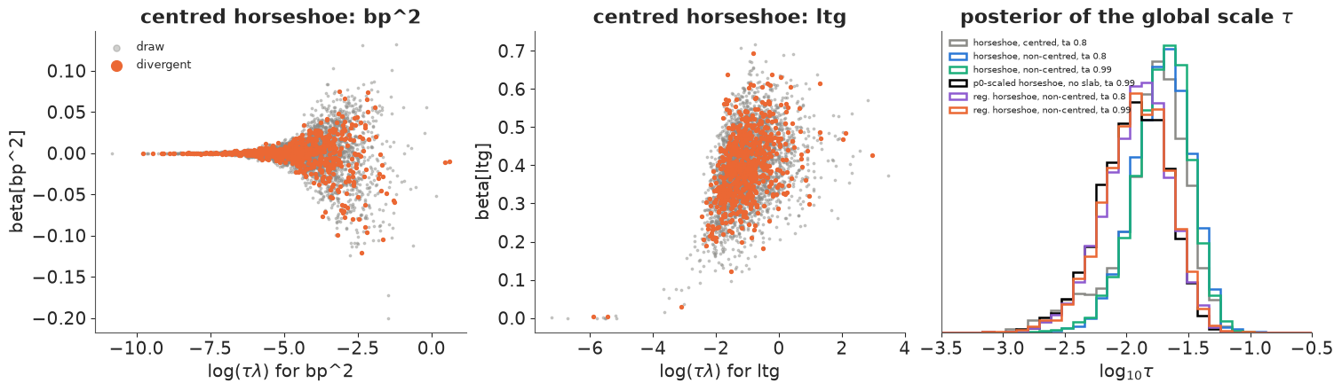
Left: the funnel for bp^2, a coefficient with nothing to say. As its scale $\tau\lambda_j$
shrinks, the coefficient is squeezed towards zero; the divergent draws (orange) are spread
along the mouth of the funnel and down its neck. Middle: ltg, a strong predictor, has no
funnel - the data pin it down - yet divergent draws show up there too, because a divergence
is a property of the whole trajectory in 64+ dimensions, not of one coordinate. Right: the
posterior of $\tau$ is much the same in every variant (the $p_0$-based ones sit a little
lower, as their prior asks). The fixes do not change the answer much; they change whether we
can trust it.
What the slab changes
The plain horseshoe has Cauchy tails: a coefficient that the data only weakly identify (here, a pair of highly correlated interactions) is allowed to wander to huge values, and the sampler has to follow $\lambda_j$ out into those tails. The regularised horseshoe replaces $\lambda_j$ by
$$\tilde\lambda_j = \sqrt{\frac{c^2\lambda_j^2}{c^2 + \tau^2\lambda_j^2}},$$
which behaves like $\lambda_j$ for small coefficients but caps the prior sd at $c$ for large ones: a horseshoe near zero, a $\text{Normal}(0, c)$ slab far from it. With $c^2 \sim \text{InvGamma}(2, 2)$ (a Student-$t_4$ slab with scale 1 on the standardised scale) no coefficient can be larger than the data can support without paying for it.
idh, idr = fits_d["horseshoe, non-centred, ta 0.99"], fits_d["reg. horseshoe, non-centred, ta 0.99"]
Bh, Br = draws(idh, "beta"), draws(idr, "beta")
order = np.argsort(-np.abs(np.median(Br, 0)))[:12]
comp = pd.DataFrame({
    "horseshoe median": np.median(Bh, 0)[order], "horseshoe 1%": np.quantile(Bh, 0.01, 0)[order],
    "horseshoe 99%": np.quantile(Bh, 0.99, 0)[order], "reg. median": np.median(Br, 0)[order],
    "reg. 1%": np.quantile(Br, 0.01, 0)[order], "reg. 99%": np.quantile(Br, 0.99, 0)[order]},
    index=np.array(NAMES)[order])
print(f"largest |beta| in any draw: horseshoe {np.abs(Bh).max():.2f}, regularised {np.abs(Br).max():.2f}")
print(f"slab scale c: median {np.median(np.sqrt(draws(idr, 'c2'))):.2f}")
comp.round(2)
largest |beta| in any draw: horseshoe 0.76, regularised 0.78
slab scale c: median 1.04
| horseshoe median | horseshoe 1% | horseshoe 99% | reg. median | reg. 1% | reg. 99% | |
|---|---|---|---|---|---|---|
| ltg | 0.40 | 0.17 | 0.61 | 0.39 | 0.18 | 0.61 |
| bmi | 0.33 | 0.09 | 0.56 | 0.35 | 0.06 | 0.54 |
| bp | 0.11 | -0.02 | 0.33 | 0.07 | -0.02 | 0.33 |
| age:sex | 0.04 | -0.03 | 0.25 | 0.02 | -0.02 | 0.25 |
| glu^2 | 0.03 | -0.03 | 0.27 | 0.02 | -0.03 | 0.29 |
| tch:glu | 0.01 | -0.05 | 0.31 | 0.00 | -0.04 | 0.26 |
| tc:tch | -0.01 | -0.33 | 0.06 | -0.00 | -0.30 | 0.05 |
| ldl:glu | 0.01 | -0.06 | 0.27 | 0.00 | -0.05 | 0.25 |
| bp:tc | 0.01 | -0.05 | 0.22 | 0.00 | -0.04 | 0.19 |
| sex:bmi | 0.01 | -0.05 | 0.18 | 0.00 | -0.04 | 0.17 |
| ldl:tch | -0.00 | -0.28 | 0.08 | -0.00 | -0.27 | 0.06 |
| sex:bp | 0.01 | -0.05 | 0.18 | 0.00 | -0.04 | 0.17 |
The slab changes little in the estimates here: the medians and the 1-99% ranges agree to
within about 0.05, and the largest coefficient in any draw is about 0.8 under both. That is
expected - the slab only binds for coefficients comparable to $c$ (median about 1), and the
biggest effect here is 0.4. It earns its place in other problems: logistic regression with
(quasi-)separation, $p > n$ designs, or correlated groups where the Cauchy tails let a
weakly identified coefficient run off. The heavy left tails of tc:tch and ldl:tch in the
table (1% quantiles near -0.3 while their medians are 0) are a milder version of that: a
correlated pair whose credit the posterior cannot assign. Section 9 looks at them.
8 · Shrinkage profiles and inclusion probabilities
The posterior of $\kappa_j$ (computed draw by draw from $\tau$, $\tilde\lambda_j$ and $\sigma$) says, per coefficient, how much the model shrinks it; the posterior of $m_\text{eff}$ is how many coefficients it effectively uses.
def kappa_draws(idata, n):
    tau, sigma, lam, c2 = (draws(idata, v) for v in ["tau", "sigma", "lam", "c2"])
    lt2 = c2[:, None] * lam**2 / (c2[:, None] + tau[:, None] ** 2 * lam**2)
    return 1 / (1 + n * tau[:, None] ** 2 * lt2 / sigma[:, None] ** 2)


K = kappa_draws(idr, n_d)
meff_post = (1 - K).sum(1)
order_k = np.argsort(np.median(K, 0))
fig, axes = plt.subplots(1, 2, figsize=(15, 4.6), gridspec_kw={"width_ratios": [2.2, 1]})
ax = axes[0]
lo, med, hi = np.quantile(K, [0.05, 0.5, 0.95], axis=0)
xs = np.arange(P_d)
ax.vlines(xs, lo[order_k], hi[order_k], color=BLUE, lw=1.5)
ax.plot(xs, med[order_k], "o", color=BLUE, ms=4)
ax.set_xticks(xs[:20])
ax.set_xticklabels(np.array(NAMES)[order_k][:20], rotation=90, fontsize=8)
ax.axhline(0.5, color=GREY, ls="--", lw=0.8)
ax.set(ylabel=r"shrinkage factor $\kappa_j$", xlabel="coefficients, least shrunk first (first 20 labelled)",
       title=r"posterior median and 90% interval of $\kappa_j$, regularised horseshoe")
ax = axes[1]
ax.hist(meff["regularised, $p_0$ = 5"], bins=64, range=(0, 64), density=True, color=GREY, alpha=0.5, label="prior")
ax.hist(meff_post, bins=64, range=(0, 64), density=True, color=ORANGE, alpha=0.8, label="posterior")
ax.set(xlabel=r"$m_\mathrm{eff}$", yticks=[], xlim=(0, 30),
       title=rf"$m_\mathrm{{eff}}$: posterior median {np.median(meff_post):.1f}")
ax.legend(fontsize=9);
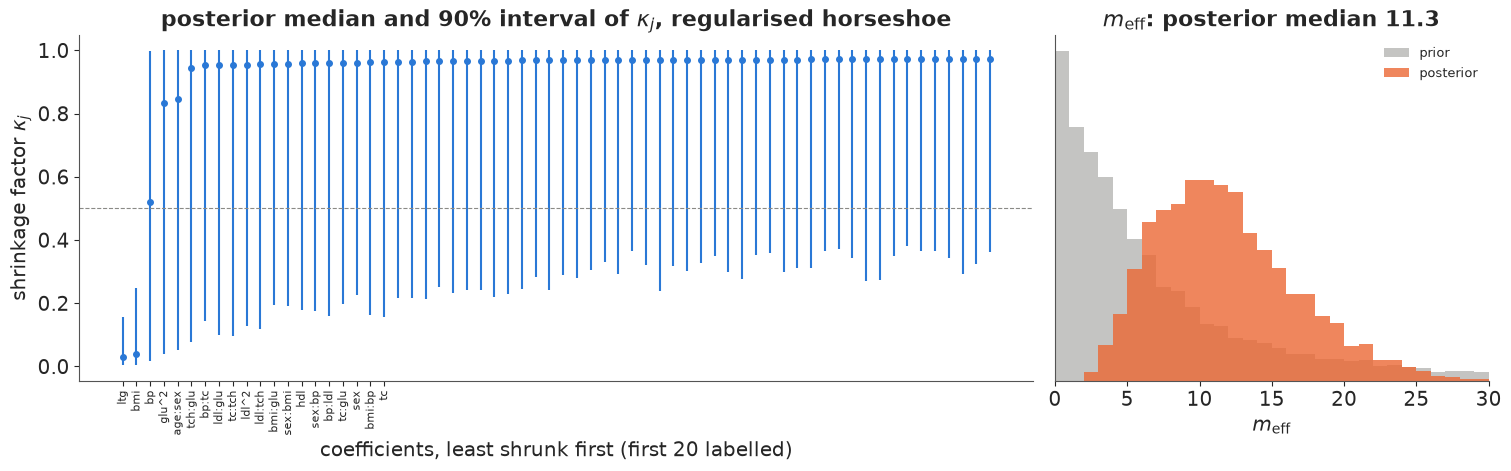
Two coefficients escape shrinkage completely (ltg and bmi, $\kappa$ near 0). bp is
half-shrunk with an interval covering almost everything. glu^2 and age:sex lean towards
shrinkage but with wide intervals; the remaining 59 have posterior median $\kappa$ around
0.94-0.97, but the lower ends of their intervals reach 0.1-0.4: in some draws each of them is
let through. That is why
$m_\text{eff}$ has a posterior median of about 11 although only two or three predictors
are clearly in: 60 coefficients that each keep a few per cent add up. (One caveat: the
$\kappa$ formula assumes roughly uncorrelated predictors, which this design is not; read it
as a shrinkage profile, not an exact decomposition.)
The horseshoe has no indicator, so it has no inclusion probability in the strict sense. The spike-and-slab does: fit it on the 64 predictors (marginalised as in section 4) and compare its PIPs with the horseshoe's $P(\kappa_j < 0.5)$, "the probability that the data outweigh the prior for this coefficient", a common stand-in.
idata_ss_d = fit(spike_slab_model(Xd_tr, yd_tr, NAMES), "diabetes, spike-and-slab", target_accept=0.95)
pip_d_draws = pip_rao_blackwell(idata_ss_d)
pip_d = pip_d_draws.mean(0)
pip_d_chain = pip_d_draws.reshape(4, -1, P_d).mean(1)
p_k = (K < 0.5).mean(0)
print(f"horseshoe P(kappa < 0.5), all 64 coefficients: min {p_k.min():.2f}, "
      f"median {np.median(p_k):.2f}, 5th largest {np.sort(p_k)[-5]:.2f}")
top = np.argsort(-np.maximum(pip_d, p_k))[:14]
pd.DataFrame({"spike-slab PIP": pip_d[top], "PIP chain min": pip_d_chain.min(0)[top],
              "PIP chain max": pip_d_chain.max(0)[top], "reg. horseshoe P(kappa<0.5)": p_k[top],
              "reg. horseshoe median beta": np.median(Br, 0)[top]}, index=np.array(NAMES)[top]).round(2)
diabetes, spike-and-slab                 2.1 s  divergences    0  max r_hat 1.488  min ess_bulk     8
horseshoe P(kappa < 0.5), all 64 coefficients: min 0.07, median 0.10, 5th largest 0.32
| spike-slab PIP | PIP chain min | PIP chain max | reg. horseshoe P(kappa<0.5) | reg. horseshoe median beta | |
|---|---|---|---|---|---|
| ltg | 1.00 | 1.00 | 1.00 | 1.00 | 0.39 |
| bmi | 0.99 | 0.97 | 1.00 | 0.99 | 0.35 |
| bp | 0.37 | 0.00 | 0.84 | 0.49 | 0.07 |
| glu^2 | 0.01 | 0.00 | 0.03 | 0.34 | 0.02 |
| ldl:glu | 0.33 | 0.00 | 0.70 | 0.18 | 0.00 |
| age:sex | 0.08 | 0.00 | 0.21 | 0.32 | 0.02 |
| tch:glu | 0.02 | 0.00 | 0.07 | 0.21 | 0.00 |
| tc:tch | 0.05 | 0.00 | 0.13 | 0.20 | -0.00 |
| ldl:tch | 0.16 | 0.00 | 0.62 | 0.17 | -0.00 |
| bp:tc | 0.01 | 0.00 | 0.03 | 0.16 | 0.00 |
| ldl^2 | 0.14 | 0.00 | 0.57 | 0.16 | -0.00 |
| bp:ldl | 0.00 | 0.00 | 0.01 | 0.14 | 0.00 |
| sex:bp | 0.03 | 0.00 | 0.11 | 0.14 | 0.00 |
| hdl | 0.00 | 0.00 | 0.01 | 0.14 | -0.00 |
The diabetes spike-and-slab is the prostate problem made worse: zero divergences, but r_hat
far above 1.1, a single-digit bulk ESS, and per-chain PIPs that disagree wildly beyond the
two obvious predictors (look at the chain min / max columns: a chain that never includes a
variable next to one that includes it most of the time). With 64 indicators there is no
enumeration to fall back on either ($2^{64}$ models). All we can take from this fit is that
ltg and bmi are in; the other numbers in its first column are Monte Carlo noise.
The horseshoe's $P(\kappa_j < 0.5)$ comes from a fit that mixes well and tells a consistent
story: ltg and bmi near 1, bp about 0.5, glu^2 and age:sex about a third, and 0.2 or
less for the rest, never 0. That is not a PIP (no coefficient is ever exactly zero under a
horseshoe), and the floor is the prior talking: its pole at $\kappa = 0$ keeps some mass on
"not shrunk" for every coefficient.
9 · Correlated predictors: how the posterior splits the credit
When two predictors carry nearly the same information, the likelihood pins down (roughly)
their sum and leaves their difference free; a sparse prior then prefers solutions in which
one of them does the work - but it does not know which one. In the diabetes data the
interactions tc:tch and ldl:tch correlate at 0.95 (total and LDL cholesterol, each times
the cholesterol ratio), and so do tc and ldl themselves at 0.94. We use the regularised
horseshoe, whose sampling we trust, and call a coefficient "relevant" in a draw when
$|\beta_j| > 0.05$ (a twentieth of an sd of the outcome per sd of the predictor).
DELTA = 0.05
pairs = [("tc:tch", "ldl:tch"), ("tc", "ldl")]
fig, axes = plt.subplots(1, 3, figsize=(15, 4.4))
rows = []
for ax, (u, v) in zip(axes[:2], pairs):
    iu_, iv_ = NAMES.index(u), NAMES.index(v)
    ru, rv = np.abs(Br[:, iu_]) > DELTA, np.abs(Br[:, iv_]) > DELTA
    rows.append((f"{u} / {v}", ru.mean(), rv.mean(), (ru | rv).mean(), (ru & rv).mean()))
    ax.scatter(Br[:, iu_], Br[:, iv_], s=3, color=ORANGE, alpha=0.3)
    ax.axhline(0, color=GREY, lw=0.8)
    ax.axvline(0, color=GREY, lw=0.8)
    ax.set(xlabel=f"beta[{u}]", ylabel=f"beta[{v}]", title=f"{u} vs {v}: r = {C[iu_, iv_]:+.2f} in the data")
    print(f"{u:>7} / {v:<7}: P(first relevant) {rows[-1][1]:.2f}, P(second) {rows[-1][2]:.2f}, "
          f"P(at least one) {rows[-1][3]:.2f}, P(both) {rows[-1][4]:.2f}; "
          f"posterior correlation of the two betas {np.corrcoef(Br[:, iu_], Br[:, iv_])[0, 1]:+.2f}")

# the same question answered exactly: prostate, all 256 models enumerated (section 4)
ax = axes[2]
lab = ["P(first)", "P(second)", "P(at least one)", "P(both)"]
for k, (u, v) in enumerate([("gleason", "pgg45"), ("svi", "lcp")]):
    gu, gv = MODELS[:, PR_NAMES.index(u)], MODELS[:, PR_NAMES.index(v)]
    vals = [w_models @ gu, w_models @ gv, w_models @ (gu | gv), w_models @ (gu & gv)]
    ax.bar(np.arange(4) + 0.38 * k, vals, width=0.36, color=[BLUE, AQUA][k], label=f"{u} / {v}")
    print(f"prostate, exact: {u} / {v}: " + ", ".join(f"{l} {x:.2f}" for l, x in zip(lab, vals)))
ax.axhline(0.5, color=GREY, ls="--", lw=0.8)
ax.set_xticks(np.arange(4) + 0.19)
ax.set_xticklabels(lab, fontsize=9)
ax.set(ylim=(0, 1), ylabel="exact posterior probability", title="prostate spike-and-slab, exact")
ax.legend(fontsize=9);
 tc:tch / ldl:tch: P(first relevant) 0.20, P(second) 0.17, P(at least one) 0.34, P(both) 0.03; posterior correlation of the two betas -0.17
     tc / ldl    : P(first relevant) 0.13, P(second) 0.10, P(at least one) 0.22, P(both) 0.01; posterior correlation of the two betas -0.18
prostate, exact: gleason / pgg45: P(first) 0.25, P(second) 0.43, P(at least one) 0.53, P(both) 0.16
prostate, exact: svi / lcp: P(first) 0.63, P(second) 0.36, P(at least one) 0.68, P(both) 0.31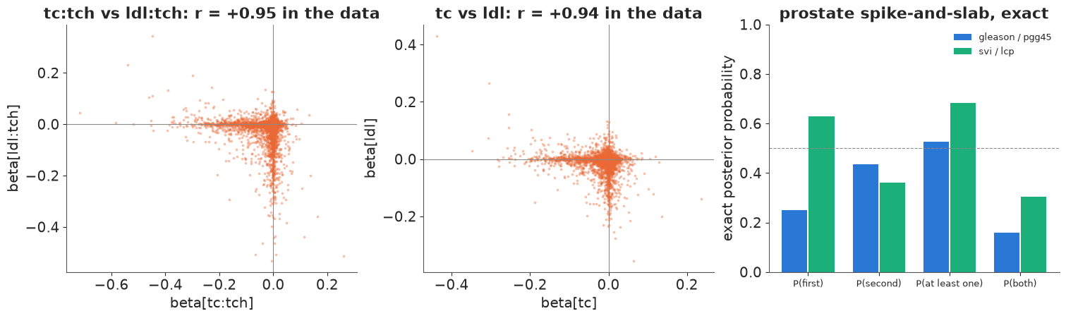
The two scatter plots are the signature of a sparse prior meeting a correlated pair: the mass
lies along the axes - one coefficient non-zero, the other at zero - and almost never in the
quadrant where both are. Each member of tc:tch / ldl:tch is "relevant" in about one draw
in five, the pair in about one in three, both together almost never. A table of marginal
probabilities (0.20 and 0.17) makes the pair look weaker than it is (0.34). And the ordinary posterior
correlation of the two coefficients is only about -0.2: the dependence is a cross, not an
ellipse, and a correlation coefficient does not see it.
The right panel asks the same question of the exact prostate posterior. Both Gleason variables have PIP below 0.5 (0.25 and 0.43), so the usual "median probability model" (keep everything with PIP above 0.5) drops both - yet the posterior probability that at least one of them belongs in the model is 0.53. The lesson is general: with correlated predictors, ask about groups (at least one of this cluster), or use a selection method that looks at predictions rather than at coefficients one at a time.
10 · From a posterior to a choice of variables: projection predictive selection
Thresholding marginal PIPs is the obvious rule, and section 9 shows why it can drop both
members of a pair that matters. Projection predictive selection (Goutis & Robert 1998;
Piironen, Paasiniemi & Vehtari 2020; the projpred R package, kulprit in Python) takes a
different route: fit the best model you can - the reference model, here the regularised
horseshoe on all 64 predictors - and then look for the smallest submodel whose predictions
are close to the reference model's.
For a Gaussian linear model the projection is ordinary least squares. For each posterior
draw $s$ the reference model's fitted means $\mu^{(s)}$ are regressed on the submodel's
columns; the projected noise is $\sigma_\perp^{(s)2} = \sigma^{(s)2} + \|\mu^{(s)} - X_S
\beta_\perp^{(s)}\|^2/n$. A forward search adds, at each step, the predictor that makes the
projection closest to the reference. kulprit is not installed here, so we write it - it is
25 lines of NumPy. The search uses the training data only; the held-out patients are used to
score each submodel size.
def gauss_elpd(y, mu, sigma):
    """Pointwise log predictive density, averaged over draws: mu (S, n), sigma (S,)."""
    lp = stats.norm.logpdf(y[None, :], mu, sigma[:, None])
    return logsumexp(lp, axis=0) - np.log(len(sigma))


def project(X, Mu, sigma, cols):
    """Project every draw's fitted mean onto the columns `cols` (plus intercept)."""
    Xs_ = np.c_[np.ones(len(X)), X[:, cols]]
    coef, *_ = np.linalg.lstsq(Xs_, Mu.T, rcond=None)                       # (k+1, S)
    resid = Mu - (Xs_ @ coef).T
    return coef, np.sqrt(sigma**2 + (resid**2).mean(1))


def forward_search(X, Mu, sigma, max_size):
    path = []
    for _ in range(max_size):
        best, best_d = None, np.inf
        for j in set(range(X.shape[1])) - set(path):
            coef, _ = project(X, Mu, sigma, path + [j])
            d = ((Mu - (np.c_[np.ones(len(X)), X[:, path + [j]]] @ coef).T) ** 2).sum()
            if d < best_d:
                best, best_d = j, d
        path.append(best)
    return path


thin = slice(None, None, 4)                                               # 1000 draws are plenty
a_r, s_r, B_r = draws(idr, "a")[thin], draws(idr, "sigma")[thin], Br[thin]
Mu_tr = a_r[:, None] + B_r @ Xd_tr.T
MAX_SIZE = 15
path = forward_search(Xd_tr, Mu_tr, s_r, MAX_SIZE)
elpd_ref = gauss_elpd(yd_te, a_r[:, None] + B_r @ Xd_te.T, s_r)
sizes, elpd_k, se_k = [0] + list(range(1, MAX_SIZE + 1)), [], []
for k in sizes:
    coef, s_perp = project(Xd_tr, Mu_tr, s_r, path[:k])
    mu_te = (np.c_[np.ones(len(Xd_te)), Xd_te[:, path[:k]]] @ coef).T
    e = gauss_elpd(yd_te, mu_te, s_perp)
    elpd_k.append(e.sum())
    se_k.append(np.sqrt(len(e)) * np.std(e - elpd_ref))
elpd_k, se_k = np.array(elpd_k), np.array(se_k)
size_sel = int(np.argmax(elpd_k - elpd_ref.sum() > -se_k))
print("search path:", ", ".join(NAMES[j] for j in path))
print(f"size 0 (intercept only): {elpd_k[0] - elpd_ref.sum():.0f} below the reference")
print(f"smallest size within one SE of the reference: {size_sel} -> {[NAMES[j] for j in path[:size_sel]]}")
search path: bmi, ltg, glu^2, bp, age:sex, ldl:tch, tch:glu, bp:tc, bmi^2, hdl, ldl:glu, tc, sex:bp, sex:tch, tc:hdl
size 0 (intercept only): -104 below the reference
smallest size within one SE of the reference: 4 -> ['bmi', 'ltg', 'glu^2', 'bp']
fig, ax = plt.subplots(figsize=(10, 4.2))
ax.errorbar(sizes, elpd_k - elpd_ref.sum(), yerr=se_k, fmt="o-", color=BLUE, capsize=3,
            label="projected submodel")
ax.axhline(0, color=ORANGE, lw=1.5, label="reference model (reg. horseshoe, 64 predictors)")
ax.axvline(size_sel, color=GREY, ls="--", lw=1)
ax.set_xticks(sizes)
ax.set_xticklabels([f"{k}\n{NAMES[path[k - 1]]}" if k else "0" for k in sizes], fontsize=7)
ax.set(ylabel="test elpd - reference elpd", xlabel="submodel size (and the predictor added)",
       ylim=(max(-80, (elpd_k - elpd_ref.sum()).min() - 10), 15),
       title="projection predictive forward search, scored on 322 held-out patients")
ax.legend(fontsize=9, loc="lower right");
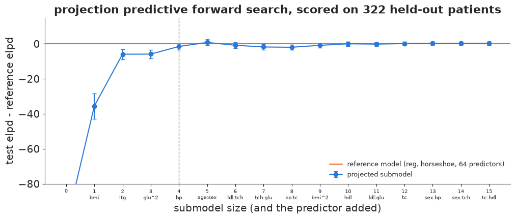
The intercept-only model is more than 100 elpd units behind the reference. Adding the
predictors in the order the search found them - bmi and ltg first, then glu^2 and bp
- closes almost all of the gap: with those four the projected model is within one standard error of the full 64-predictor reference, and from five on the curve stays within about 2 elpd of it. The four chosen predictors are body-mass index, blood pressure, log triglycerides and squared glucose - the last one ranked fourth by the horseshoe's $P(\kappa < 0.5)$ and missed entirely by the (badly mixed) spike-and-slab.
Two honest caveats. (1) We chose the size by looking at the test set; projpred does it
by cross-validation on the training data (with the search repeated inside each fold, since a
search that saw the data is optimistic), which is the right way when there is no spare test
set. (2) Forward search is greedy, and with correlated predictors the order among the
near-duplicates is somewhat arbitrary - but projection solves the problem of section 9: a
submodel that contains tc:tch does not need ldl:tch, and the search knows that because it
measures predictions, not coefficients.
11 · The frequentist reference: lasso with cross-validation
Coordinate descent for the lasso is a dozen lines: cycle through the coefficients, soft-threshold each partial residual correlation, repeat until nothing moves. A path of 50 penalties from the one that zeroes everything down to 1% of it, with warm starts and 10-fold cross-validation, takes a few seconds. (Going further down the path is slow and pointless here: with 64 collinear columns and 108 rows per fold, coordinate descent crawls when the penalty is tiny, and cross-validation has long stopped improving.)
def lasso_cd(X, y, lam, b=None, tol=1e-6, max_iter=5000):
    """Coordinate descent on the Gram matrix for (1/2n)||y - Xb||^2 + lam ||b||_1."""
    n, P = X.shape
    G, c = X.T @ X / n, X.T @ y / n
    b = np.zeros(P) if b is None else b.copy()
    Gb = G @ b
    for _ in range(max_iter):
        delta = 0.0
        for j in range(P):
            old = b[j]
            rho = c[j] - Gb[j] + G[j, j] * old                  # partial-residual correlation
            new = np.sign(rho) * max(abs(rho) - lam, 0.0) / G[j, j]
            if new != old:
                Gb += G[:, j] * (new - old)
                b[j] = new
                delta = max(delta, abs(new - old))
        if delta < tol:
            break
    return b


def lasso_path(X, y, lams):
    xm, ym = X.mean(0), y.mean()
    b, out = None, []
    for lam in lams:
        b = lasso_cd(X - xm, y - ym, lam, b)
        out.append((ym - xm @ b, b.copy()))
    return out


t0 = time.time()
lam_max = np.abs(Xd_tr.T @ (yd_tr - yd_tr.mean())).max() / n_d
lams = lam_max * np.logspace(0, -2, 50)
folds = rng.permutation(n_d) % 10
cv = np.zeros((10, len(lams)))
for f in range(10):
    fit_path = lasso_path(Xd_tr[folds != f], yd_tr[folds != f], lams)
    for k, (a0, b) in enumerate(fit_path):
        cv[f, k] = np.mean((yd_tr[folds == f] - a0 - Xd_tr[folds == f] @ b) ** 2)
cv_mean, cv_se = cv.mean(0), cv.std(0) / np.sqrt(10)
k_min = int(np.argmin(cv_mean))
k_1se = int(np.argmax(cv_mean <= cv_mean[k_min] + cv_se[k_min]))
full_path = lasso_path(Xd_tr, yd_tr, lams)
lasso_min, lasso_1se = full_path[k_min], full_path[k_1se]
print(f"lasso path + 10-fold CV: {time.time() - t0:.1f} s; lambda_min is penalty {k_min + 1} of {len(lams)}, "
      f"lambda_1se is {k_1se + 1}")
for label, (a0, b) in [("lambda_min", lasso_min), ("lambda_1se", lasso_1se)]:
    nz = np.flatnonzero(b)
    print(f"lasso {label}: {len(nz)} non-zero: {', '.join(NAMES[j] for j in nz[np.argsort(-np.abs(b[nz]))])}")
lasso path + 10-fold CV: 4.3 s; lambda_min is penalty 20 of 50, lambda_1se is 13
lasso lambda_min: 8 non-zero: ltg, bmi, bp, glu^2, age:sex, hdl, bmi^2, tc:tch
lasso lambda_1se: 4 non-zero: ltg, bmi, bp, glu^2
At the penalty that minimises cross-validated error ($\lambda_\text{min}$) the lasso keeps
8 predictors; at the largest penalty within one standard error of that minimum
($\lambda_\text{1se}$, the usual "sparser but as good" rule) it keeps 4 - ltg, bmi,
bp and glu^2, the same four that the projection chose. Two quite different routes to
the same answer is reassuring. The lasso gives no uncertainty about that choice, though; the
posterior does (the size-by-size curve above, and the $\kappa$ intervals).
12 · Held-out predictive performance
Finally, the question that does not depend on anyone's definition of "selected": how well does each fit predict the 322 patients it has not seen? We report the root mean squared error of the posterior mean prediction and the log predictive density (elpd) in the original units of the progress score. For least squares and the lasso the elpd is a plug-in Normal with the training residual sd (so it ignores estimation uncertainty and flatters them a little).
fits_d["ridge"] = fit(sparse_lm(Xd_tr, yd_tr, "ridge", NAMES), "ridge", target_accept=0.9)
fits_d["Bayesian lasso"] = fit(sparse_lm(Xd_tr, yd_tr, "lasso", NAMES), "Bayesian lasso", target_accept=0.9)


def score_bayes(a, B, sigma, X, y):
    """Test RMSE (original units) and pointwise test log predictive density (original units)."""
    mu = a[:, None] + B @ X.T
    rmse = np.sqrt(np.mean((mu.mean(0) - y) ** 2)) * yd_sd
    return rmse, gauss_elpd(y, mu, sigma) - np.log(yd_sd)


def score_plugin(a0, b, X_tr, y_tr, X, y):
    resid_sd = np.std(y_tr - a0 - X_tr @ b)
    mu = a0 + X @ b
    rmse = np.sqrt(np.mean((mu - y) ** 2)) * yd_sd
    return rmse, stats.norm.logpdf(y, mu, resid_sd) - np.log(yd_sd)


rows = {}
coef_ols = np.linalg.lstsq(np.c_[np.ones(n_d), Xd_tr], yd_tr, rcond=None)[0]
rows["least squares, 64 predictors"] = score_plugin(coef_ols[0], coef_ols[1:], Xd_tr, yd_tr, Xd_te, yd_te)
coef_10 = np.linalg.lstsq(np.c_[np.ones(n_d), Xd_tr[:, :10]], yd_tr, rcond=None)[0]
rows["least squares, 10 main effects"] = score_plugin(coef_10[0], coef_10[1:], Xd_tr[:, :10], yd_tr, Xd_te[:, :10], yd_te)
rows["lasso, lambda_min"] = score_plugin(*lasso_min, Xd_tr, yd_tr, Xd_te, yd_te)
rows["lasso, lambda_1se"] = score_plugin(*lasso_1se, Xd_tr, yd_tr, Xd_te, yd_te)
for label in ["ridge", "Bayesian lasso", "horseshoe, non-centred, ta 0.99", "reg. horseshoe, non-centred, ta 0.99"]:
    i = fits_d[label]
    rows[label] = score_bayes(draws(i, "a"), draws(i, "beta"), draws(i, "sigma"), Xd_te, yd_te)
rows["spike-and-slab"] = score_bayes(draws(idata_ss_d, "a"), draws(idata_ss_d, "beta"), draws(idata_ss_d, "sigma"),
                                     Xd_te, yd_te)
coef, s_perp = project(Xd_tr, Mu_tr, s_r, path[:size_sel])
rows[f"projection, {size_sel} predictors"] = score_bayes(
    coef[0], coef[1:].T, s_perp, Xd_te[:, path[:size_sel]], yd_te)
ref_pw = rows["reg. horseshoe, non-centred, ta 0.99"][1]
res = pd.DataFrame({label: {"test RMSE": r, "test elpd": pw.sum(), "elpd - reg. horseshoe": (pw - ref_pw).sum(),
                            "SE of difference": np.sqrt(len(pw)) * np.std(pw - ref_pw)}
                    for label, (r, pw) in rows.items()}).T
print("main effects, least squares (10 predictors) vs reg. horseshoe median (64 predictors):")
print(pd.DataFrame({"least squares": coef_10[1:], "reg. horseshoe": np.median(Br[:, :10], 0)}, index=MAIN).round(2).T)
res.round(1)
ridge 0.8 s divergences 0 max r_hat 1.003 min ess_bulk 1582
Bayesian lasso                           1.0 s  divergences    0  max r_hat 1.004  min ess_bulk   946
main effects, least squares (10 predictors) vs reg. horseshoe median (64 predictors):
                 age   sex   bmi    bp    tc   ldl   hdl   tch   ltg   glu
least squares  -0.01 -0.14  0.33  0.21 -0.75  0.39  0.27  0.26  0.58  0.06
reg. horseshoe 0.00 -0.00 0.35 0.07 -0.00 -0.00 -0.00 0.00 0.39 0.00| test RMSE | test elpd | elpd - reg. horseshoe | SE of difference | |
|---|---|---|---|---|
| least squares, 64 predictors | 137.1 | -4080.2 | -2331.3 | 717.4 |
| least squares, 10 main effects | 54.0 | -1741.7 | 7.1 | 5.9 |
| lasso, lambda_min | 54.0 | -1741.8 | 7.1 | 2.7 |
| lasso, lambda_1se | 56.3 | -1757.2 | -8.3 | 4.3 |
| ridge | 56.8 | -1762.4 | -13.6 | 4.6 |
| Bayesian lasso | 55.6 | -1755.4 | -6.6 | 3.1 |
| horseshoe, non-centred, ta 0.99 | 54.6 | -1749.5 | -0.6 | 0.7 |
| reg. horseshoe, non-centred, ta 0.99 | 54.4 | -1748.9 | 0.0 | 0.0 |
| spike-and-slab | 55.0 | -1751.5 | -2.6 | 2.0 |
| projection, 4 predictors | 54.7 | -1750.3 | -1.5 | 2.1 |
What the table says, in order of confidence:
- Least squares with 64 predictors is a disaster (RMSE 137 on an outcome whose sd is about 77): this is the problem that shrinkage solves. Every shrinkage method gets to an RMSE of 54-57.
- The horseshoes beat ridge clearly (about 14 elpd, about 3 standard errors) and the Bayesian lasso by about 2 standard errors. Plain and regularised horseshoe predict the same, and the projected 4-predictor submodel loses only 1.5 (SE 2). The lasso at $\lambda_\text{1se}$ has the same four predictors but loses about 8: its penalty shrinks the four coefficients that it keeps, while the projection fits them to the reference model's predictions without further shrinkage.
- The surprise: the lasso at $\lambda_\text{min}$ and plain least squares on the 10 main
effects are better than the regularised horseshoe, by about 7 elpd (0.02 per patient;
RMSE 54.0 against 54.4). For the lasso the difference is about 2.5 standard errors, so it
is probably not noise; for the main-effects model it is only 1.2. (The plug-in elpd
flatters the two point estimates somewhat, so the real gap is a little smaller.) The printed main effects show the likely reason. Least squares on the
10 main effects uses a contrast of the correlated cholesterol measurements (
tc-0.75,ldl+0.39,hdl+0.27,tch+0.26) plussexand a largerbp; the horseshoe sets all the cholesterol terms andsexto zero and keepsbpat a third of the size. A contrast of correlated predictors is exactly what a sparse prior finds expensive (section 9): several non-zero coefficients where one would almost do. On 120 patients the data are not strong enough to overrule $p_0 = 5$. The horseshoe is not automatically the best predictor; it is a good default when you believe in sparsity, and a held-out set (or LOO) is how you find out whether you should. - The spike-and-slab predicts about as well as the others despite its sampling problems: prediction averages over the confusion about which correlated variable is in, which matters little for $\hat y$. Its PIPs, not its predictions, are what the poor mixing ruins.
13 · Summary
| Question | Answer in this notebook |
|---|---|
| Why not a Normal prior? | It shrinks every coefficient by the same factor ($\kappa$ fixed): noise is kept and signal is shrunk |
| Is the Bayesian lasso sparse? | Its mode is (that is the lasso); its posterior is not - no pole at zero, and one rate for noise and signal |
| What makes the horseshoe work? | A U-shaped prior on $\kappa$: each coefficient is either shrunk away or left alone |
| How to set $\tau$? | From a guess $p_0$: $\tau_0 = \frac{p_0}{P-p_0}\frac{\sigma}{\sqrt n}$; check the implied prior on $m_\text{eff}$ by simulation. HalfCauchy(1) says "almost everything is non-zero" |
| Divergences? | Non-centre, raise target_accept, use the regularised horseshoe (scale + slab): all three together took ~650 to 1 |
| Spike-and-slab with NUTS? | Only the continuous relaxation, indicators summed out one at a time; no divergences but poor mixing between in and out - check r_hat per chain, enumerate when $P$ is small |
| Correlated predictors? | The posterior splits the credit along the axes; marginal inclusion probabilities undercount a correlated pair - ask about groups |
| Which variables? | Projection predictive selection: smallest submodel whose predictions match the reference. Here bmi, ltg, bp, glu^2 - as the lasso at $\lambda_\text{1se}$ |
| Does it predict better? | Much better than least squares and ridge; not better than the CV lasso or a main-effects model on this split - check, do not assume |
Try it yourself
- p > n. Refit sections 7-12 on 50 training patients instead of 120 (so $P = 64 > n$).
Least squares is no longer defined; which of the priors degrade gracefully, and does the
projection still find
ltg,bmiandbpfirst? - Sensitivity to $p_0$. Refit the regularised horseshoe with $p_0 = 1$ and $p_0 = 20$ and overlay the posteriors of $m_\text{eff}$ on their priors. How much does the posterior move with the prior guess on 120 patients - and on all 442?
- A real high-dimensional problem. The riboflavin data (Bühlmann, Kalisch & Meier 2014;
R package
hdi) has $n = 71$ and $P = 4088$ gene expressions. Screen to the 500 genes most correlated with the response (and say why screening on the training data biases what follows), fit the regularised horseshoe with $p_0 = 10$, and compare the projection path with the lasso's.