A marketing mix model (MMM) turns weekly spend by channel into an estimate of what each channel adds, and the only reason anyone builds one is to move money. Two open-source designs dominate practice: Google's Meridian and PyMC-Marketing. Both share a core:
- carry-over (adstock): an ad seen this week still sells next week;
- saturation: the 100th thousand euros buys fewer customers than the first;
- geo hierarchy (Meridian's headline feature): fit many markets at once and let the response curves of each market be partially pooled toward a channel-wide curve, because one market's history is rarely enough to pin down a curve on its own;
- priors on business quantities (Meridian's ROI priors): say what you believe about cost per customer, not about a coefficient on an arbitrary scale.
This notebook builds that core from scratch in about 60 lines of PyMC, so every piece is visible and changeable, and then does what the model is for: a budget reallocation across channels x markets at a fixed total, with the uncertainty carried all the way to the decision. It is the second notebook of a media-measurement series. E32 showed that spend which chases demand biases every MMM, including this one; section 8 comes back to that.
import json
import logging
from pathlib import Path

import arviz as az
import matplotlib.pyplot as plt
import numpy as np
import pandas as pd
import pymc as pm
import pytensor.tensor as pt
import matplotlib.dates as mdates
import seaborn as sns
from matplotlib.patches import Ellipse
from scipy.optimize import minimize

from pymc_challenges import data

RANDOM_SEED = 42
rng = np.random.default_rng(RANDOM_SEED)
az.style.use("arviz-variat")
logging.getLogger("pymc").setLevel(logging.WARNING)  # eleven fits: no sampler banner per fit
BLUE, ORANGE, AQUA, GREY, PURPLE = "#2a78d6", "#eb6834", "#1baf7a", "#8a8a86", "#8c5ac8"
CH_COLOR = {"Google": BLUE, "Meta": ORANGE}
print(f"PyMC {pm.__version__}, ArviZ {az.__version__}")
PyMC 6.3.2, ArviZ 1.3.0
1 · The brief and the choice of data
"We sell in Denmark, Sweden and Norway and split paid media between Google and Meta. Next year's paid budget is the same as this year's. Should we move money between channels or markets, how many extra new customers would that buy, and how sure are you?"
- Head of Growth, a Scandinavian apparel brand
Conjura's dataset has 143 brand x territory daily series. A multi-market model needs one brand with several real markets (the "All Territories" rows are sums of the others, not a market), each with both Google and Meta spend on most days, for at least a year and a half (fewer than two seasonal cycles already makes the baseline hard). A quick scan:
data.describe("conjura_mmm")
raw = data.load("conjura_mmm")
raw["date"] = pd.to_datetime(raw["DATE_DAY"])
raw["google"] = raw.filter(regex="^GOOGLE.*_SPEND").fillna(0).sum(axis=1)
raw["meta"] = raw.filter(regex="^META.*_SPEND").fillna(0).sum(axis=1)
terr = raw[raw["TERRITORY_NAME"] != "All Territories"]
scan = terr.groupby(["ORGANISATION_ID", "TERRITORY_NAME"]).agg(
    vertical=("ORGANISATION_VERTICAL", "first"), days=("date", "size"),
    new_cust_per_day=("FIRST_PURCHASES", "mean"),
    google_days=("google", lambda s: (s > 0).mean()), meta_days=("meta", lambda s: (s > 0).mean()))
ok = scan[(scan["days"] >= 540) & (scan["google_days"] > 0.9) & (scan["meta_days"] > 0.9)]
n_ok = ok.groupby(level=0).size()
print("brands with >= 2 markets that each have >= 540 days and Google AND Meta on > 90% of days:")
ok.loc[n_ok[n_ok >= 2].index].round(2)
conjura_mmm: 132,759 brand x territory x day rows (143 anonymised series from 93 e-commerce brands, 2019-2024): first-time and all purchases (orders, units, original price, discount), and spend / clicks / impressions for Google (search, shopping, PMax, display, video), Meta (Facebook, Instagram, other) and TikTok, plus organic/direct/email/referral clicks. Missing spend means the brand did not use that channel.
  source: Anderson, A. (2024), Multi-Region Marketing Mix Modelling (MMM) Dataset for Several eCommerce Brands, Conjura, figshare, doi:10.6084/m9.figshare.25314841 (CC BY 4.0).
  url:    https://ndownloader.figshare.com/files/46779652
brands with >= 2 markets that each have >= 540 days and Google AND Meta on > 90% of days:
| vertical | days | new_cust_per_day | google_days | meta_days | ||
|---|---|---|---|---|---|---|
| ORGANISATION_ID | TERRITORY_NAME | |||||
| 4a762f02ca755b22d37393e8dbeab1a6 | UK | Apparel | 941 | 27.23 | 0.99 | 1.00 |
| US | Apparel | 1029 | 92.62 | 0.99 | 1.00 | |
| 7569a6a9c156a0f9398fa6cfd51df5bb | Canada | Food & Drink | 821 | 13.03 | 1.00 | 0.94 |
| US | Food & Drink | 821 | 204.39 | 1.00 | 1.00 | |
| c5fbe353800204351f2768f90d703b38 | Denmark | Apparel | 571 | 117.12 | 1.00 | 0.99 |
| Norway | Apparel | 571 | 8.58 | 1.00 | 0.99 | |
| Sweden | Apparel | 571 | 19.49 | 1.00 | 0.99 | |
| f7e5ba45e3e337e8e90787ae0218a7ac | UK | Home & Garden | 1088 | 44.58 | 1.00 | 0.97 |
| US | Home & Garden | 701 | 13.14 | 0.95 | 0.95 |
Only one brand qualifies with three markets: a Danish apparel brand selling in Denmark, Sweden and Norway, all three on the same 571 days with both channels running almost every day. (The nearest alternative, a German sports brand in Germany, Austria and Switzerland, runs Meta on only about 80% of days at a tenth of its Google spend; the brands with more markets barely use Meta outside the UK. The "several brands of one vertical in one territory" alternative gives at most two brands per territory.) Three markets is the minimum for a hierarchy to be worth anything, and a hierarchical variance estimated from three groups is mostly prior - that will matter.
Two data decisions, stated up front:
- Weekly aggregation (Monday-Sunday, full weeks only: 81 weeks). Budgets are planned weekly, carry-over is measured in weeks, and daily data mainly add day-of-week noise and autocorrelated residuals that make a posterior look more certain than it is.
- One currency. A reallocation between markets has to compare a krone in Oslo with a krone in Copenhagen, so spend is converted to euros at fixed ECB 2023 average reference rates (EUR 1 = DKK 7.4509 = SEK 11.4788 = NOK 11.4248). A fixed rate only rescales each market's spend, so it changes nothing within a market; the 2023 average is the right rate for a plan that will be paid for next year at roughly current rates.
ORG = "c5fbe353800204351f2768f90d703b38"
MARKETS, CHANNELS = ["Denmark", "Sweden", "Norway"], ["Google", "Meta"]
FX = {"DKK": 7.4509, "SEK": 11.4788, "NOK": 11.4248}  # ECB reference rates, 2023 averages
d = terr[terr["ORGANISATION_ID"] == ORG].copy()
d["Google"] = d["google"] / d["CURRENCY_CODE"].map(FX)
d["Meta"] = d["meta"] / d["CURRENCY_CODE"].map(FX)
d = d[(d["date"] >= "2022-10-31") & (d["date"] <= "2024-05-19")]  # full Monday-Sunday weeks
wk = d.groupby(["TERRITORY_NAME", pd.Grouper(key="date", freq="W-SUN")])[
    ["FIRST_PURCHASES", "Google", "Meta"]].sum()
weeks = wk.loc["Denmark"].index  # week-ending Sundays
T, M, C = len(weeks), len(MARKETS), len(CHANNELS)
Y = np.stack([wk.loc[m]["FIRST_PURCHASES"].to_numpy() for m in MARKETS])  # (market, week)
S = np.stack([np.stack([wk.loc[m][c].to_numpy() for c in CHANNELS]) for m in MARKETS])  # EUR
print(f"{T} weeks, {weeks[0].date()} -> {weeks[-1].date()}")
pd.DataFrame({"new customers / week": Y.mean(axis=1).round(0),
              "Google EUR / week": S[:, 0].mean(axis=1).round(0),
              "Meta EUR / week": S[:, 1].mean(axis=1).round(0),
              "blended CAC (EUR)": (S.sum(axis=(1, 2)) / Y.sum(axis=1)).round(1),
              "corr(Google, Meta)": [np.corrcoef(S[i])[0, 1].round(2) for i in range(M)]},
             index=MARKETS)
81 weeks, 2022-11-06 -> 2024-05-19
| new customers / week | Google EUR / week | Meta EUR / week | blended CAC (EUR) | corr(Google, Meta) | |
|---|---|---|---|---|---|
| Denmark | 824.0 | 4602.0 | 7072.0 | 14.2 | 0.84 |
| Sweden | 137.0 | 1333.0 | 1656.0 | 21.8 | 0.68 |
| Norway | 60.0 | 554.0 | 822.0 | 22.8 | 0.60 |
fig, axes = plt.subplots(3, 1, figsize=(11, 8), sharex=True)
for i, (ax, m) in enumerate(zip(axes, MARKETS)):
    ax.plot(weeks, Y[i], color="k", lw=1.5, label="new customers")
    ax.set_ylabel("new customers / week")
    ax2 = ax.twinx()
    for j, c in enumerate(CHANNELS):
        ax2.plot(weeks, S[i, j] / 1000, color=CH_COLOR[c], lw=1, alpha=0.8, label=f"{c} spend")
    ax2.set_ylabel("spend (EUR 000 / week)")
    ax2.grid(False)
    ax.set_title(m, loc="left", fontsize=10)
    for yr in (2022, 2023):
        ax.axvspan(pd.Timestamp(f"{yr}-11-21"), pd.Timestamp(f"{yr}-12-24"), color=PURPLE, alpha=0.1)
axes[0].legend(loc="upper center", fontsize=8)
ax2.legend(loc="upper right", fontsize=8)
fig.suptitle("New customers and paid spend by market (shaded: Black Friday to Christmas)");
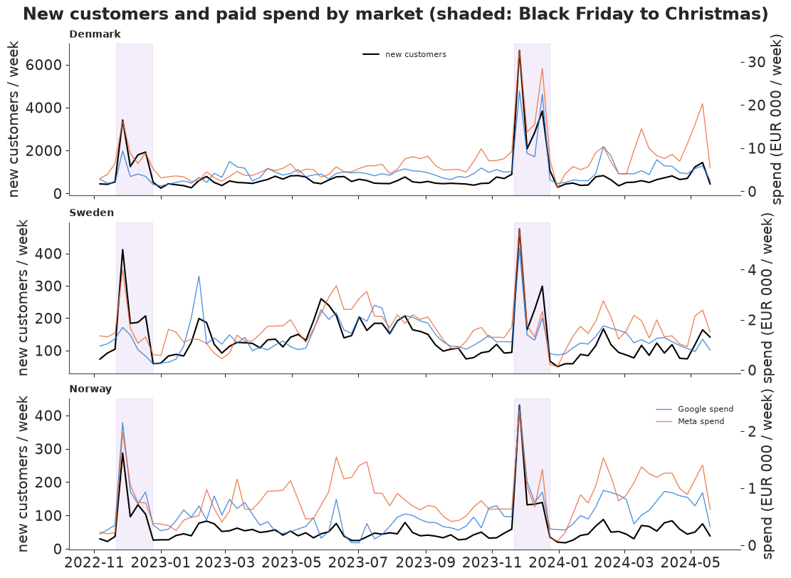
What a modeller should see here:
- Scale. Denmark is the home market: about 14 times Norway's new customers and 8 times its spend. Norway averages about 60 new customers a week - a small market, where one market's data will not pin down two response curves.
- Black Friday and the Christmas run-up dominate everything: customers jump five- to eight-fold and spend jumps with them. If the model has no other explanation for those weeks, it will credit them to media. So the baseline gets explicit holiday controls.
- Google and Meta move together (correlation 0.84 in Denmark): the data alone can only weakly tell the two channels apart. That is the classic MMM identification problem, and one thing a hierarchy can help with.
- The blended cost per customer (all spend / all new customers) is 14-23 euros. That is an upper bound on what media could possibly deliver, not an estimate of it: some customers would have come anyway.
2 · The model
For market $m$, channel $c$, week $t$, with $x_{mct}$ = spend in units of that cell's average week:
Adstock (carry-over over $L = 6$ weeks, normalised geometric weights): $a_{mct} = \sum_{\ell=0}^{5} w_\ell\, x_{mc,t-\ell}$, $w_\ell \propto \theta_{mc}^\ell$.
Saturation (Hill curve with slope 1, Meridian's default for media, i.e. concave): the channel adds $\beta_{mc}\, a/(a + k_{mc})$ new customers a week, where $k_{mc}$ is the half-saturation point in units of average spend and $\beta_{mc}$ the ceiling.
Priors in business units. Rather than a prior on $\beta$ (whose scale depends on the market's size), the model is parameterised by $\text{cpc}_{mc}$, the cost per incremental customer at the cell's average spend (euros). At average spend ($a = 1$) the channel adds $\beta/(1+k)$ customers a week for $\bar S_{mc}$ euros, so $\beta_{mc} = (\bar S_{mc}/ \text{cpc}_{mc})(1 + k_{mc})$. This is Meridian's ROI-prior idea: a marketer can say "a customer bought by paid media probably costs between 15 and 170 euros", while nobody has a feeling for $\beta$. And cost per customer in euros is a quantity that is plausibly exchangeable across markets of one brand - the right scale on which to pool.
Partial pooling (non-centred): $\log \text{cpc}_{mc} = \mu^{\text{cpc}}_c + \sigma^{\text{cpc}} z_{mc}$, and the same for $\log k_{mc}$ and $\text{logit}\,\theta_{mc}$, with $z \sim N(0, 1)$. Each channel has its own average across markets; how far a market may stray is learnt.
Baseline (the customers who would have come anyway), per market: $\bar y_m \exp(b_m + \text{trend}_m t + \text{season}_m(t) + \text{holiday}_m(t))$, with two yearly Fourier harmonics partially pooled across markets and three holiday indicators - Black Friday week, the Christmas run-up weeks, and the holiday lull (weeks ending 24 Dec - 7 Jan) - also partially pooled. Media adds customers on top of the baseline, so "customers bought by media" is well defined.
Likelihood: $y_{mt} \sim \text{NegativeBinomial}(\text{baseline}_{mt} + \sum_c \text{media}_{mct},\ \alpha_m)$.
L_ADSTOCK = 6
HOLIDAYS = ["black_friday", "christmas_run_up", "holiday_lull"]
H = np.zeros((len(HOLIDAYS), T))
for bf in pd.to_datetime(["2022-11-25", "2023-11-24"]):
    i_bf = np.searchsorted(weeks, bf)  # the week (ending Sunday) that contains Black Friday
    H[0, i_bf] = 1
    for i in range(i_bf + 1, T):
        if weeks[i].month == 12 and weeks[i].day >= 24:
            break
        H[1, i] = 1
H[2] = [(w.month == 12 and w.day >= 24) or (w.month == 1 and w.day <= 7) for w in weeks]
for h, name in enumerate(HOLIDAYS):
    print(f"{name:17s}", [w.strftime("%d %b %y") for w in weeks[H[h] == 1]])

t_years = np.arange(T) * 7 / 365.25
doy = weeks.dayofyear.to_numpy() / 365.25
FOURIER = np.column_stack([f(2 * np.pi * k * doy) for k in (1, 2) for f in (np.sin, np.cos)])
S_MEAN = S.mean(axis=2)  # EUR per average week, (market, channel)
Y_MEAN = Y.mean(axis=1)
XS = S / S_MEAN[..., None]  # spend in units of the cell's average week
LAG = np.arange(T)[:, None] + (L_ADSTOCK - 1) - np.arange(L_ADSTOCK)[None, :]
# before the first week, assume spend continued at the first week's level
XLAG = np.concatenate([np.repeat(XS[..., :1], L_ADSTOCK - 1, axis=2), XS], axis=2)[..., LAG]


def adstock(theta):
    """theta (market, channel) -> adstocked spend (market, channel, week). XLAG is (m, c, t, lag)."""
    w = theta[..., None] ** pt.arange(L_ADSTOCK)
    w = w / w.sum(axis=-1, keepdims=True)
    return (XLAG * w[:, :, None, :]).sum(axis=-1)
black_friday      ['27 Nov 22', '26 Nov 23']
christmas_run_up  ['04 Dec 22', '11 Dec 22', '18 Dec 22', '03 Dec 23', '10 Dec 23', '17 Dec 23']
holiday_lull      ['25 Dec 22', '01 Jan 23', '24 Dec 23', '31 Dec 23', '07 Jan 24']
One function builds all the variants used below: pooling is "partial", "none" (every
cell on its own, with the same marginal prior the hierarchy implies, so the comparison is
only about pooling) or "full" (one curve per channel for all markets). The prior arguments
are there for the sensitivity analysis of section 8.
SD_SCALE = {"cpc": 0.4, "k": 0.4, "theta": 0.5}  # half-normal scales of between-market sds


def build_mmm(pooling="partial", cpc_prior=(np.log(50.0), 0.7), k_prior=(np.log(1.5), 0.5),
              centred=False, sd_scale=SD_SCALE):
    coords = {"market": MARKETS, "channel": CHANNELS, "week": weeks, "holiday": HOLIDAYS,
              "fourier": ["sin1", "cos1", "sin2", "cos2"]}
    mc = ("market", "channel")
    with pm.Model(coords=coords) as model:
        # ---- media: channel-level means ...
        mu_cpc = pm.Normal("mu_log_cpc", cpc_prior[0], cpc_prior[1], dims="channel")
        mu_k = pm.Normal("mu_log_k", k_prior[0], k_prior[1], dims="channel")
        mu_th = pm.Normal("mu_logit_theta", -0.5, 0.8, dims="channel")
        # ... and market-level deviations
        if pooling == "partial":
            sd = {v: pm.HalfNormal(f"sd_{v}", sd_scale[v]) for v in sd_scale}
            if centred:
                log_cpc = pm.Normal("log_cpc", mu_cpc, sd["cpc"], dims=mc)
            else:
                log_cpc = mu_cpc + sd["cpc"] * pm.Normal("z_cpc", 0, 1, dims=mc)
            log_k = mu_k + sd["k"] * pm.Normal("z_k", 0, 1, dims=mc)
            logit_th = mu_th + sd["theta"] * pm.Normal("z_theta", 0, 1, dims=mc)
        elif pooling == "none":  # same marginal prior per cell, no sharing
            log_cpc = pm.Normal("log_cpc", cpc_prior[0], np.hypot(cpc_prior[1], SD_SCALE["cpc"]), dims=mc)
            log_k = pm.Normal("log_k", k_prior[0], np.hypot(k_prior[1], SD_SCALE["k"]), dims=mc)
            logit_th = pm.Normal("logit_theta", -0.5, np.hypot(0.8, SD_SCALE["theta"]), dims=mc)
        else:  # full pooling: one curve per channel
            log_cpc, log_k, logit_th = (pt.broadcast_to(v, (M, C)) for v in (mu_cpc, mu_k, mu_th))
        cpc = pm.Deterministic("cpc", pt.exp(log_cpc), dims=mc)
        k = pm.Deterministic("k", pt.exp(log_k), dims=mc)
        theta = pm.Deterministic("theta", pm.math.sigmoid(logit_th), dims=mc)
        beta = pm.Deterministic("beta", S_MEAN / cpc * (1 + k), dims=mc)  # customers/week ceiling
        a = adstock(theta)
        media = pm.Deterministic("media", beta[..., None] * a / (a + k[..., None]),
                                 dims=("market", "channel", "week"))
        # ---- baseline
        b0 = pm.Normal("b0", np.log(0.6), 0.5, dims="market")
        trend = pm.Normal("trend", 0.0, 0.5, dims="market")
        season = (pm.Normal("season_mu", 0.0, 0.3, dims="fourier")
                  + pm.HalfNormal("season_sd", 0.1) * pm.Normal("season_z", 0, 1, dims=("market", "fourier")))
        holiday = (pm.Normal("holiday_mu", 0.0, 1.0, dims="holiday")
                   + pm.HalfNormal("holiday_sd", 0.3) * pm.Normal("holiday_z", 0, 1, dims=("market", "holiday")))
        eta = b0[:, None] + trend[:, None] * t_years + pt.dot(season, FOURIER.T) + pt.dot(holiday, H)
        baseline = pm.Deterministic("baseline", Y_MEAN[:, None] * pt.exp(eta), dims=("market", "week"))
        alpha = pm.Gamma("alpha", 2.0, 0.1, dims="market")
        pm.NegativeBinomial("y", mu=baseline + media.sum(axis=1), alpha=alpha[:, None],
                            observed=Y, dims=("market", "week"))
    return model


def fit(model, label, **kw):
    """Sample, keeping only free variables and the small media parameters (not media/baseline)."""
    keep = [v.name for v in model.free_RVs] + ["cpc", "k", "theta", "beta"]
    kw = {"target_accept": 0.95, **kw}
    idata = pm.sample(model=model, random_seed=RANDOM_SEED, progressbar=False, var_names=keep, **kw)
    print(f"  {label}: divergences = {int(idata.sample_stats['diverging'].sum())}, "
          f"tuning steps = {idata.posterior.attrs.get('tuning_steps')}")
    return idata


def summary(idata, names, **kw):
    """az.summary one variable at a time: in ArviZ 1.3 a multi-variable call can mislabel
    rows when variables share a dimension (see the gotcha in the text)."""
    return pd.concat([az.summary(idata, var_names=[v], **kw) for v in names])
The prior on cost per incremental customer is centred on 50 euros with a log-sd of 0.7 (90% of the prior mass between about 16 and 160 euros for a channel's average; each market can stray further). That is deliberately generous: it allows media to be almost as cheap as the blended cost (every customer bought by ads) and allows it to be ten times dearer (hardly any). The half-saturation point is centred on 1.5 times current average spend (concave, but with room to grow), and adstock decay on about 0.4 per week.
3 · Prior predictive check, in euros
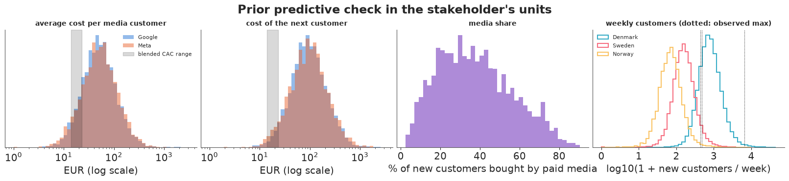
A prior predictive check should be read in the units the stakeholder uses. Four questions: what cost per customer does the prior allow, what marginal cost of the next customer, what share of new customers does it attribute to paid media, and are the implied weekly customer numbers anywhere near reality?
m_partial = build_mmm("partial")
prior = pm.sample_prior_predictive(model=m_partial, draws=1000, random_seed=RANDOM_SEED,
                                   var_names=["cpc", "k", "theta", "beta", "media", "baseline", "y"])


def draws_of(idata, names, group="posterior", n=1000, seed=RANDOM_SEED):
    """Dict of NumPy arrays with the sample dimension first."""
    ex = az.extract(idata, group=group, var_names=list(names), num_samples=n, random_seed=seed)
    return {v: ex[v].transpose("sample", ...).to_numpy() for v in names}


def adstock_np(theta):
    """theta (draws, market, channel) -> (draws, market, channel, week)."""
    w = theta[..., None] ** np.arange(L_ADSTOCK)
    w = w / w.sum(axis=-1, keepdims=True)
    return np.einsum("mctl,dmcl->dmct", XLAG, w)


def marginal_cost(p, r=None, last=52):
    """EUR per EXTRA customer for a small spend increase in each cell, over the last `last` weeks
    of spend scaled by r (market, channel). d/dr of beta*r*a/(r*a + k) is beta*a*k/(r*a + k)**2."""
    r = np.ones((M, C)) if r is None else r
    a = adstock_np(p["theta"])[..., -last:]
    ra = r[..., None] * a
    d_customers = (p["beta"][..., None] * a * p["k"][..., None] / (ra + p["k"][..., None]) ** 2).sum(-1)
    return S[..., -last:].sum(-1) / d_customers  # (draws, market, channel)


pp = draws_of(prior, ["cpc", "k", "theta", "beta", "media", "baseline"], group="prior")
pp_y = az.extract(prior, group="prior_predictive", var_names=["y"], num_samples=1000,
                  random_seed=RANDOM_SEED).transpose("sample", ...).to_numpy()  # one name: a DataArray
media_share = pp["media"].sum(axis=(2, 3)) / (pp["media"].sum(axis=(2, 3)) + pp["baseline"].sum(axis=2))
mcost_prior = marginal_cost(pp, last=T)

fig, axes = plt.subplots(1, 4, figsize=(16, 3.6))
bins = np.logspace(0, np.log10(3000), 50)
for j, c in enumerate(CHANNELS):
    axes[0].hist(pp["cpc"][:, :, j].ravel(), bins=bins, color=CH_COLOR[c], alpha=0.5, label=c)
    axes[1].hist(mcost_prior[:, :, j].ravel(), bins=bins, color=CH_COLOR[c], alpha=0.5, label=c)
for ax, title in zip(axes[:2], ["average cost per media customer", "cost of the next customer"]):
    ax.set(xscale="log", xlabel="EUR (log scale)", yticks=[])
    ax.set_title(title, fontsize=10)
    ax.axvspan(14, 23, color="k", alpha=0.15, label="blended CAC range")
axes[0].legend(fontsize=8)
axes[2].hist(100 * media_share.ravel(), bins=40, color=PURPLE, alpha=0.7)
axes[2].set(xlabel="% of new customers bought by paid media", yticks=[])
axes[2].set_title("media share", fontsize=10)
for i, m in enumerate(MARKETS):
    axes[3].hist(np.log10(pp_y[:, i].ravel() + 1), bins=50, histtype="step", lw=1.5, label=m)
    axes[3].axvline(np.log10(Y[i].max() + 1), color="k", lw=0.8, ls=":")
axes[3].set(xlabel="log10(1 + new customers / week)", yticks=[])
axes[3].set_title("weekly customers (dotted: observed max)", fontsize=10)
axes[3].legend(fontsize=8)
fig.suptitle("Prior predictive check in the stakeholder's units");
print("prior media share of new customers, 5/50/95%:", np.quantile(100 * media_share, [0.05, 0.5, 0.95]).round(0))
print("prior marginal cost per customer, 5/50/95%: ", np.quantile(mcost_prior, [0.05, 0.5, 0.95]).round(0))
for i, m in enumerate(MARKETS):
    print(f"{m:8s} weekly customers, prior 5/50/95%: {np.quantile(pp_y[:, i], [0.05, 0.5, 0.95]).round(0)}"
          f" | observed {Y[i].min()}-{Y[i].max()}")
prior media share of new customers, 5/50/95%: [10. 36. 72.]
prior marginal cost per customer, 5/50/95%:  [ 24.  94. 373.]
Denmark  weekly customers, prior 5/50/95%: [ 260.  769. 2652.] | observed 251-6662
Sweden   weekly customers, prior 5/50/95%: [ 54. 156. 489.] | observed 50-476
Norway   weekly customers, prior 5/50/95%: [ 23.  69. 219.] | observed 18-431
The prior knows the order of magnitude and little else, which is what it should know:
- Average cost per media customer sits mostly between 15 and 200 euros. Only a small fraction of draws fall below the blended CAC (grey band), which would mean paid media bought nearly all new customers on its own - possible for one channel, implausible for both.
- The cost of the next customer is higher (median about 90 euros) because the curves are concave: the prior already says "the next euro works less hard than the average euro".
- Media share is spread from about 10% to 70% of new customers: the prior takes no side in the "is marketing doing anything?" argument - the data will have to.
- Weekly customers land on the right scale in every market; the observed holiday peaks (dotted) are in the upper tail, as they should be for a prior that has not seen them.
4 · Fitting: centred vs non-centred
With three markets, the between-market sd of log cost per customer is estimated from three numbers, and the data allow it to be very small. That is the setting for Neal's funnel: in the centred form the six market-level costs are sampled directly around the channel mean, and when the sd is small they are squeezed into a narrow neck the sampler cannot enter. The non-centred form samples standardised deviations $z$ instead.
idata_centred = fit(build_mmm("partial", centred=True), "centred, target_accept 0.8", target_accept=0.8)
idata_nc80 = fit(m_partial, "non-centred, target_accept 0.8", target_accept=0.8)
idata = fit(m_partial, "non-centred, target_accept 0.95")
for lab, idt in [("centred", idata_centred), ("non-centred", idata_nc80), ("non-c., 0.95", idata)]:
    print(f"{lab:12s} sd_cpc: ESS bulk = {float(az.ess(idt.posterior['sd_cpc'])):.0f}, "
          f"r_hat = {float(az.rhat(idt.posterior['sd_cpc'])):.3f}; "
          f"max r_hat over cpc = {float(az.rhat(idt.posterior['cpc']).max()):.3f}")
centred, target_accept 0.8: divergences = 59, tuning steps = 400
non-centred, target_accept 0.8: divergences = 105, tuning steps = 400
  non-centred, target_accept 0.95: divergences = 1, tuning steps = 400
centred      sd_cpc: ESS bulk = 499, r_hat = 1.007; max r_hat over cpc = 1.003
non-centred  sd_cpc: ESS bulk = 210, r_hat = 1.015; max r_hat over cpc = 1.010
non-c., 0.95 sd_cpc: ESS bulk = 583, r_hat = 1.005; max r_hat over cpc = 1.005
fig, axes = plt.subplots(1, 3, figsize=(14, 3.8), sharey=True)
for ax, (lab, idt) in zip(axes, [("centred, target_accept 0.8", idata_centred),
                                 ("non-centred, target_accept 0.8", idata_nc80),
                                 ("non-centred, target_accept 0.95", idata)]):
    sdv = idt.posterior["sd_cpc"].values.ravel()
    cv = np.log(idt.posterior["cpc"].sel(market="Norway", channel="Meta").values.ravel())
    dv = idt.sample_stats["diverging"].values.ravel().astype(bool)
    ax.scatter(cv[~dv], np.log(sdv[~dv]), s=3, alpha=0.3, color=GREY)
    ax.scatter(cv[dv], np.log(sdv[dv]), s=12, color=ORANGE, label=f"divergent ({dv.sum()})")
    ax.set(xlabel="log cost per customer, Norway Meta", title=lab)
    ax.legend(fontsize=8)
axes[0].set_ylabel("log between-market sd of log cost");
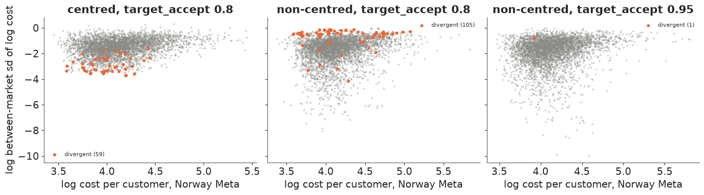
The three panels are one posterior explored three ways, and the two parameterisations fail at opposite ends of it:
- Centred (left): the divergences sit in the neck of the funnel, at small between-market sd, and the draws stop well short of the region the non-centred sampler visits. The part of the posterior where the three markets are nearly identical is cut off: a bias toward less pooling that r_hat does not flag.
- Non-centred at the default step size (middle): the neck is explored freely, but the divergences move to the top - large between-market sd, where the markets decouple and, as in the unpooled fit of section 6, Denmark's two co-moving channels can trade credit along a narrow curved ridge. No reparameterisation removes that curvature.
- Non-centred with
target_accept=0.95(right): a smaller step size gets round the ridge, leaving at most a handful of divergences.
(The exact counts change from run to run - nutpie is not bit-reproducible - but where the divergences sit does not.) Non-centred plus a smaller step is the fit used from here on.
Diagnostics of the non-centred fit (default nutpie settings apart from target_accept=0.95):
del idata_centred, idata_nc80
summary(idata, ["mu_log_cpc", "mu_log_k", "mu_logit_theta", "sd_cpc", "sd_k", "sd_theta",
                "cpc", "k", "theta", "holiday_mu", "trend", "alpha"], round_to=2)
| mean | sd | eti89_lb | eti89_ub | ess_bulk | ess_tail | r_hat | mcse_mean | mcse_sd | |
|---|---|---|---|---|---|---|---|---|---|
| mu_log_cpc[Google] | 3.19 | 0.21 | 2.89 | 3.58 | 792.34 | 835.35 | 1.01 | 0.01 | 0.01 |
| mu_log_cpc[Meta] | 4.02 | 0.29 | 3.61 | 4.51 | 1243.11 | 1609.08 | 1.00 | 0.01 | 0.01 |
| mu_log_k[Google] | 1.32 | 0.43 | 0.62 | 2.00 | 4775.60 | 3159.22 | 1.00 | 0.01 | 0.01 |
| mu_log_k[Meta] | 0.92 | 0.46 | 0.17 | 1.63 | 5297.18 | 3056.67 | 1.00 | 0.01 | 0.01 |
| mu_logit_theta[Google] | -1.36 | 0.49 | -2.15 | -0.61 | 4678.75 | 3066.93 | 1.00 | 0.01 | 0.01 |
| mu_logit_theta[Meta] | -1.58 | 0.61 | -2.56 | -0.63 | 5517.29 | 3486.12 | 1.00 | 0.01 | 0.01 |
| sd_cpc | 0.24 | 0.17 | 0.02 | 0.54 | 583.14 | 657.35 | 1.01 | 0.01 | 0.00 |
| sd_k | 0.46 | 0.32 | 0.04 | 1.04 | 1730.93 | 1499.90 | 1.00 | 0.01 | 0.00 |
| sd_theta | 0.37 | 0.28 | 0.03 | 0.89 | 2649.65 | 1964.13 | 1.00 | 0.00 | 0.00 |
| cpc[Denmark, Google] | 23.58 | 6.72 | 15.98 | 34.82 | 1615.66 | 1630.34 | 1.00 | 0.18 | 0.32 |
| cpc[Denmark, Meta] | 49.57 | 20.92 | 26.51 | 82.42 | 1034.31 | 1547.49 | 1.01 | 0.63 | 1.58 |
| cpc[Sweden, Google] | 23.00 | 3.57 | 18.20 | 29.16 | 2306.16 | 2269.91 | 1.00 | 0.07 | 0.08 |
| cpc[Sweden, Meta] | 62.19 | 25.54 | 38.90 | 98.46 | 1913.42 | 2080.13 | 1.00 | 0.73 | 2.55 |
| cpc[Norway, Google] | 26.21 | 5.58 | 19.61 | 35.71 | 1496.59 | 2002.83 | 1.00 | 0.14 | 0.17 |
| cpc[Norway, Meta] | 65.81 | 23.47 | 42.26 | 104.35 | 2165.80 | 2371.78 | 1.00 | 0.54 | 1.38 |
| k[Denmark, Google] | 6.38 | 6.81 | 1.95 | 14.61 | 4690.15 | 3452.94 | 1.00 | 0.10 | 0.53 |
| k[Denmark, Meta] | 5.11 | 6.63 | 1.29 | 12.71 | 3362.28 | 3278.73 | 1.00 | 0.10 | 0.47 |
| k[Sweden, Google] | 7.13 | 6.69 | 2.51 | 16.17 | 3766.11 | 3005.76 | 1.00 | 0.10 | 0.49 |
| k[Sweden, Meta] | 3.56 | 3.86 | 0.92 | 8.19 | 4964.08 | 3202.34 | 1.00 | 0.07 | 0.38 |
| k[Norway, Google] | 6.15 | 7.12 | 2.07 | 13.67 | 4972.74 | 3928.40 | 1.00 | 0.11 | 1.06 |
| k[Norway, Meta] | 3.66 | 4.93 | 1.06 | 8.14 | 5067.23 | 3312.75 | 1.00 | 0.08 | 0.83 |
| theta[Denmark, Google] | 0.21 | 0.09 | 0.09 | 0.36 | 5094.65 | 3448.71 | 1.00 | 0.00 | 0.00 |
| theta[Denmark, Meta] | 0.17 | 0.09 | 0.05 | 0.33 | 4772.68 | 3291.72 | 1.00 | 0.00 | 0.00 |
| theta[Sweden, Google] | 0.21 | 0.09 | 0.09 | 0.37 | 4458.92 | 3378.62 | 1.00 | 0.00 | 0.00 |
| theta[Sweden, Meta] | 0.18 | 0.10 | 0.05 | 0.36 | 4567.47 | 2974.16 | 1.00 | 0.00 | 0.00 |
| theta[Norway, Google] | 0.19 | 0.08 | 0.08 | 0.32 | 5716.37 | 3548.17 | 1.00 | 0.00 | 0.00 |
| theta[Norway, Meta] | 0.18 | 0.09 | 0.06 | 0.35 | 5053.20 | 2757.67 | 1.00 | 0.00 | 0.00 |
| holiday_mu[black_friday] | 2.64 | 0.25 | 2.24 | 3.02 | 1806.06 | 2011.69 | 1.00 | 0.01 | 0.01 |
| holiday_mu[christmas_run_up] | 1.60 | 0.21 | 1.27 | 1.93 | 1906.17 | 2091.19 | 1.00 | 0.00 | 0.00 |
| holiday_mu[holiday_lull] | -0.48 | 0.28 | -0.95 | -0.08 | 2779.17 | 2414.96 | 1.00 | 0.01 | 0.01 |
| trend[Denmark] | 0.08 | 0.13 | -0.14 | 0.28 | 2651.21 | 2563.72 | 1.00 | 0.00 | 0.00 |
| trend[Sweden] | -0.39 | 0.14 | -0.62 | -0.18 | 3939.48 | 2680.33 | 1.00 | 0.00 | 0.00 |
| trend[Norway] | -0.11 | 0.16 | -0.37 | 0.13 | 3547.87 | 2734.95 | 1.00 | 0.00 | 0.00 |
| alpha[Denmark] | 18.98 | 3.16 | 14.28 | 24.38 | 4172.48 | 3139.51 | 1.00 | 0.05 | 0.05 |
| alpha[Sweden] | 37.38 | 7.90 | 25.85 | 50.97 | 4479.15 | 2991.85 | 1.00 | 0.12 | 0.15 |
| alpha[Norway] | 26.44 | 6.26 | 17.87 | 37.34 | 4858.55 | 3306.36 | 1.00 | 0.09 | 0.11 |
rhat_max = max(float(az.rhat(idata.posterior[v]).max()) for v in idata.posterior.data_vars)
ess_min = min(float(az.ess(idata.posterior[v]).min()) for v in idata.posterior.data_vars)
print(f"all parameters: max r_hat = {rhat_max:.3f}, min bulk ESS = {ess_min:.0f}, "
      f"divergences = {int(idata.sample_stats['diverging'].sum())}")
all parameters: max r_hat = 1.005, min bulk ESS = 583, divergences = 1
All r_hat are at most 1.01 and the smallest bulk ESS (the between-market sd of cost) is several hundred. What the parameters say:
- Cost per incremental customer at average spend: Google's channel average is about exp(3.2) = 24 euros, Meta's about exp(4.0) = 55 euros, with each market close to its channel average (the between-market sd of log cost is small, about 0.25).
- Saturation is weakly identified: half-saturation points of roughly 3-7 times average spend with 90% intervals from about 1 to 15. The observed spend range shows only gentle curvature, so where the curves flatten is partly the prior's call - section 8 tests it.
- Carry-over is short: a weekly decay near 0.2, so most of the effect lands in the week of spend.
- Holidays: the Black Friday week multiplies the baseline about 14-fold (exp(2.6)) and the Christmas run-up about 5-fold; the holiday lull is below normal. Without these controls, all of that would be available to be credited to the spend that rose with it.
5 · Posterior predictive check and the decomposition
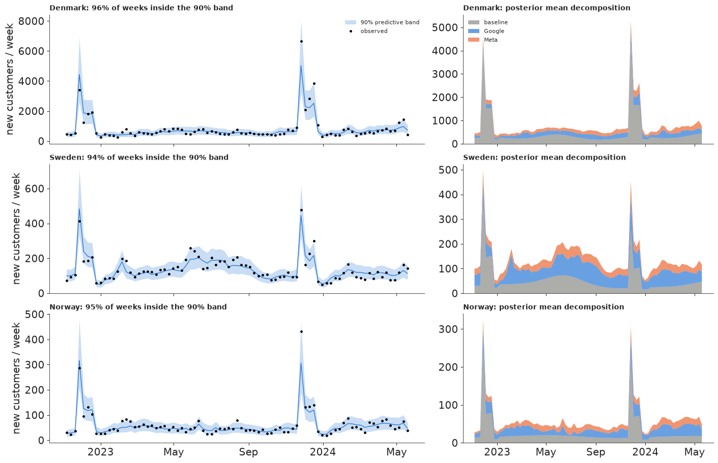
Does the model reproduce the weekly series, including the holiday spikes and Norway's noise? And how does it split each week into "would have come anyway" and "bought by Google / Meta"?
thin = idata.isel(draw=slice(None, None, 4))
ppc = pm.sample_posterior_predictive(thin, model=m_partial, var_names=["y", "media", "baseline"],
                                     random_seed=RANDOM_SEED, progressbar=False)
yrep = ppc.posterior_predictive["y"].stack(s=("chain", "draw")).transpose("s", ...).to_numpy()
media_post = ppc.posterior_predictive["media"].mean(("chain", "draw")).to_numpy()  # (m, c, t)
base_post = ppc.posterior_predictive["baseline"].mean(("chain", "draw")).to_numpy()
lo, hi = np.quantile(yrep, [0.05, 0.95], axis=0)
cover = ((Y >= lo) & (Y <= hi)).mean(axis=1)

fig, axes = plt.subplots(3, 2, figsize=(14, 9), sharex=True, gridspec_kw={"width_ratios": [3, 2]})
for i, m in enumerate(MARKETS):
    ax = axes[i, 0]
    ax.fill_between(weeks, lo[i], hi[i], color=BLUE, alpha=0.25, lw=0, label="90% predictive band")
    ax.plot(weeks, np.median(yrep[:, i], axis=0), color=BLUE, lw=1)
    ax.plot(weeks, Y[i], "o", color="k", ms=2.5, label="observed")
    ax.set_title(f"{m}: {100 * cover[i]:.0f}% of weeks inside the 90% band", loc="left", fontsize=10)
    ax.set_ylabel("new customers / week")
    ax = axes[i, 1]
    ax.stackplot(weeks, base_post[i], media_post[i, 0], media_post[i, 1],
                 colors=[GREY, BLUE, ORANGE], alpha=0.7, labels=["baseline", "Google", "Meta"])
    ax.set_title(f"{m}: posterior mean decomposition", loc="left", fontsize=10)
for ax in axes[-1]:
    loc = mdates.MonthLocator(bymonth=[1, 5, 9])
    ax.xaxis.set_major_locator(loc)
    ax.xaxis.set_major_formatter(mdates.ConciseDateFormatter(loc))
axes[0, 0].legend(fontsize=8)
axes[0, 1].legend(fontsize=8, loc="upper left");
share = media_post.sum(axis=2) / (media_post.sum(axis=(1, 2)) + base_post.sum(axis=1))[:, None]
pd.DataFrame(100 * share, index=MARKETS, columns=[f"% of new customers from {c}" for c in CHANNELS]).round(0)
| % of new customers from Google | % of new customers from Meta | |
|---|---|---|
| Denmark | 24.0 | 19.0 |
| Sweden | 42.0 | 21.0 |
| Norway | 35.0 | 22.0 |
The 90% predictive bands contain 94-96% of the weeks in each market, including both Black Friday peaks, so the model is, if anything, slightly cautious. The decomposition is the MMM's actual claim: paid media bought roughly 45% of Denmark's new customers and about 55-65% of Sweden's and Norway's, with Google carrying the larger share everywhere. Look at Sweden's summer 2023 bump: new customers rose, Google spend rose with it, and the model gives most of the bump to Google. That is either Google working, or Google's bidding following a demand surge - the pattern E32 is about, and one this model cannot tell apart (section 8).
6 · What pooling buys - and what LOO does not see
Fit the same model with no pooling (each of the six cells on its own, with the same marginal prior) and with full pooling (one curve per channel for all three markets).
m_none, m_full = build_mmm("none"), build_mmm("full")
idata_none = fit(m_none, "no pooling")
idata_full = fit(m_full, "full pooling")


def q(idt, v, qs=(0.05, 0.5, 0.95)):
    return idt.posterior[v].quantile(list(qs), dim=("chain", "draw")).to_numpy()  # (q, m, c)


cpc_tab = {}
for lab, idt in [("no pooling", idata_none), ("partial", idata), ("full pooling", idata_full)]:
    qq = q(idt, "cpc")
    cpc_tab[lab] = pd.DataFrame({f"{m} {c}": f"{qq[1, i, j]:.0f} [{qq[0, i, j]:.0f}, {qq[2, i, j]:.0f}]"
                                 for i, m in enumerate(MARKETS) for j, c in enumerate(CHANNELS)},
                                index=[lab]).T
print("average cost per incremental customer, EUR: median [90% interval]")
pd.concat(cpc_tab.values(), axis=1)
no pooling: divergences = 0, tuning steps = 400
  full pooling: divergences = 0, tuning steps = 400
average cost per incremental customer, EUR: median [90% interval]
| no pooling | partial | full pooling | |
|---|---|---|---|
| Denmark Google | 37 [18, 130] | 22 [16, 35] | 23 [19, 29] |
| Denmark Meta | 26 [19, 48] | 46 [26, 84] | 58 [42, 97] |
| Sweden Google | 22 [17, 31] | 23 [18, 29] | 23 [19, 29] |
| Sweden Meta | 63 [38, 150] | 57 [39, 100] | 58 [42, 97] |
| Norway Google | 27 [19, 50] | 25 [20, 36] | 23 [19, 29] |
| Norway Meta | 78 [42, 196] | 60 [42, 107] | 58 [42, 97] |
grid_mult = np.linspace(0, 2.5, 80)  # sustained weekly spend, multiples of the cell's average


def curves(idt, n=400):
    """Steady-state customers / week on the grid: (draws, market, channel, grid)."""
    p = draws_of(idt, ["beta", "k"], n=n)
    g = grid_mult[None, None, None, :]
    return p["beta"][..., None] * g / (g + p["k"][..., None])


cur_none, cur_part, cur_full = curves(idata_none), curves(idata), curves(idata_full)
fig, axes = plt.subplots(2, 3, figsize=(14, 7))
for i, m in enumerate(MARKETS):
    for j, c in enumerate(CHANNELS):
        ax = axes[j, i]
        spend_axis = grid_mult * S_MEAN[i, j]
        for cv, col, lab in [(cur_none, GREY, "own data only"), (cur_part, CH_COLOR[c], "partial pooling"),
                             (cur_full, "k", "one curve for all")]:
            lo_, med_, hi_ = np.quantile(cv[:, i, j], [0.05, 0.5, 0.95], axis=0)
            if col == "k":
                ax.plot(spend_axis, med_, color="k", ls="--", lw=1, label=lab)
            else:
                ax.fill_between(spend_axis, lo_, hi_, color=col, alpha=0.25, lw=0)
                ax.plot(spend_axis, med_, color=col, lw=1.5, label=lab)
        ax.axvline(S_MEAN[i, j], color=GREY, ls=":")
        ax.set_title(f"{m} · {c}", fontsize=10, loc="left")
        ax.set_xlabel("sustained spend (EUR / week)")
    axes[0, i].legend(fontsize=7) if i == 0 else None
fig.supylabel("new customers / week from the channel")
fig.suptitle("Response curves, 90% bands (dotted: average spend over the 81 weeks)");
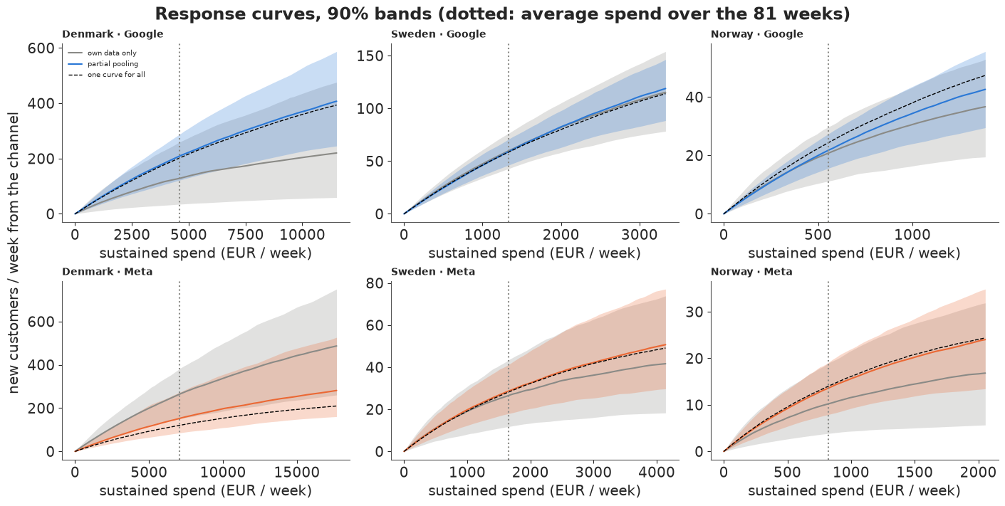
Two ways to go wrong without pooling, both visible in the table and the grey bands:
- The small market is simply uncertain. Norway's Meta curve on its own data allows anything from a nearly flat curve to a steep one: a cost per customer of about 40 to 200 euros. One market's 81 weeks cannot pin down two curves when a week brings about 60 new customers.
- The large market gets the split wrong. Denmark has plenty of data, but Google and Meta move together there (correlation 0.84), so on its own it can only estimate their sum. The unpooled fit hands the credit the other way round from every other market (Meta cheaper than Google) with a Google interval running to over 100 euros. Pooling does not add data about Denmark; it adds the information that in the markets where the two channels can be told apart, Google is the cheaper one.
Partial pooling pulls both back toward the channel average and narrows the intervals. Full pooling (dashed) goes further and forces one curve on all markets; partial pooling ends up close to it here because the data favour a small between-market sd - but it let the data decide that, and keeps Denmark's Meta somewhat cheaper than the others.
Does LOO prefer the hierarchy? All three models give a per-week likelihood, so PSIS-LOO compares them directly.
loos = {}
for lab, idt, mdl in [("partial", idata, m_partial), ("no pooling", idata_none, m_none),
                      ("full pooling", idata_full, m_full)]:
    pm.compute_log_likelihood(idt, model=mdl, progressbar=False)
    loos[lab] = az.loo(idt, pointwise=True)
    loos[lab].log_weights = None
    del idt["log_likelihood"]
    bad = loos[lab].pareto_k.to_series()
    bad = bad[bad > 0.7]
    print(f"{lab:13s}: Pareto k > 0.7 for {len(bad)} of {M * T} weeks:",
          [f"{m} {pd.Timestamp(w):%d %b %y}" for m, w in bad.index])
az.compare(loos, round_to=1)
partial : Pareto k > 0.7 for 2 of 243 weeks: ['Sweden 27 Nov 22', 'Norway 26 Nov 23']
no pooling : Pareto k > 0.7 for 2 of 243 weeks: ['Denmark 26 Nov 23', 'Norway 26 Nov 23']
full pooling : Pareto k > 0.7 for 3 of 243 weeks: ['Denmark 26 Nov 23', 'Norway 27 Nov 22', 'Norway 26 Nov 23']
| rank | elpd_diff | dse | p_worse | diag_diff | diag_elpd | p | elpd | se | weight | |
|---|---|---|---|---|---|---|---|---|---|---|
| partial | 0 | 0.0 | 0.0 | NaN | 2 k̂ > 0.70 | 29.3 | -1226.7 | 22.3 | 1.0 | |
| full pooling | 1 | -1.5 | 1.2 | 0.9 | |elpd_diff| < 4 | 3 k̂ > 0.70 | 27.6 | -1228.2 | 22.5 | 0.0 |
| no pooling | 2 | -3.3 | 2.6 | 0.9 | |elpd_diff| < 4 | 2 k̂ > 0.70 | 30.7 | -1230.0 | 22.2 | 0.0 |
LOO ranks partial pooling first, but the differences are within about one standard error: by predictive fit alone, the three models are indistinguishable. That is not a failure of LOO but a fact about MMMs worth knowing. Week-to-week new customers are driven mostly by the baseline and the holidays, and the total media contribution is similar across the three models; what differs is how that total is split between channels and markets - and two co-moving channels can split a total many ways with almost the same fit (the unpooled Denmark estimate is exactly that). LOO scores predictions of new customers, not the correctness of an attribution. The case for the hierarchy is structural (markets of one brand are exchangeable) and practical (stabler curves, and a decision that does not rest on one market's collinearity). The two or three weeks with high Pareto k, listed above, are Black Friday weeks: each is most of the evidence for its own market's Black Friday effect, so leaving it out changes the fit - expected, and too few to distort the comparison.
7 · The decision: reallocating a fixed budget
The plan space. Next year's budget equals the last 52 weeks' spend in every cell. A plan multiplies each of the six cells' spend by a factor $r_{mc}$, keeping the week-to-week pattern (Black Friday pushes and all), with the total fixed. Each factor is kept between 0.5 and 1.5: the curves are only informed near the spend levels actually observed, and a plan that moves further than that is extrapolation, not estimation (PyMC-Marketing's optimiser has the same budget bounds for the same reason).
The objective. Because adstock is linear, scaling a cell's spend by $r$ scales its adstocked spend by $r$, so the customers a plan buys over the year are, for every posterior draw, $\sum_{m,c,t} \beta_{mc}\, r_{mc} a_{mct} / (r_{mc} a_{mct} + k_{mc})$. The optimiser (SLSQP) maximises either the posterior mean of the extra customers, or a cautious objective, mean minus 1.65 posterior sds (roughly the 5th percentile of the gain). The chosen plan is then evaluated over all posterior draws.
LAST = 52
BUDGET = S[..., -LAST:].sum(axis=-1)  # EUR per cell over the last 52 weeks
post = draws_of(idata, ["beta", "k", "theta"])


class Planner:
    """Customers bought by media over the last 52 weeks' pattern, for any spend multipliers."""

    def __init__(self, p):
        self.beta, self.k = p["beta"][..., None], p["k"][..., None]
        self.a = adstock_np(p["theta"])[..., -LAST:]
        self.now = self.customers(np.ones((M, C)))

    def customers(self, r):
        ra = np.reshape(r, (M, C))[..., None] * self.a
        return (self.beta * ra / (ra + self.k)).sum(axis=(1, 2, 3))

    def gain(self, r):
        return self.customers(r) - self.now

    def optimise(self, risk=0.0):
        def objective(v):
            g = self.gain(v)
            return -(g.mean() - risk * g.std()) / 1000

        budget = {"type": "eq", "fun": lambda v: v @ BUDGET.ravel() / BUDGET.sum() - 1}
        res = minimize(objective, np.ones(M * C), method="SLSQP", bounds=[(0.5, 1.5)] * (M * C),
                       constraints=[budget], options={"ftol": 1e-12, "maxiter": 500})
        assert res.success, res.message
        return res.x.reshape(M, C)


planner = Planner(post)
plan_mean = planner.optimise(risk=0.0)
plan_safe = planner.optimise(risk=1.65)
mcost_now = marginal_cost(post)

table = pd.DataFrame(index=pd.MultiIndex.from_product([MARKETS, CHANNELS], names=["market", "channel"]))
table["spend now (EUR 000/yr)"] = (BUDGET.ravel() / 1000).round(0)
table["marginal cost now (EUR)"] = [f"{np.median(v):.0f} [{np.quantile(v, 0.05):.0f}, {np.quantile(v, 0.95):.0f}]"
                                    for v in mcost_now.reshape(len(mcost_now), -1).T]
table["best-guess plan (EUR 000)"] = (plan_mean.ravel() * BUDGET.ravel() / 1000).round(0)
table["cautious plan (EUR 000)"] = (plan_safe.ravel() * BUDGET.ravel() / 1000).round(0)
table
| spend now (EUR 000/yr) | marginal cost now (EUR) | best-guess plan (EUR 000) | cautious plan (EUR 000) | ||
|---|---|---|---|---|---|
| market | channel | ||||
| Denmark | 269.0 | 30 [21, 53] | 403.0 | 299.0 | |
| Meta | 430.0 | 69 [35, 147] | 313.0 | 421.0 | |
| Sweden | 76.0 | 28 [22, 40] | 114.0 | 114.0 | |
| Meta | 95.0 | 89 [55, 182] | 47.0 | 47.0 | |
| Norway | 29.0 | 33 [25, 51] | 44.0 | 39.0 | |
| Meta | 47.0 | 93 [61, 181] | 24.0 | 24.0 |
def describe_plan(r, label):
    g = planner.gain(r)
    return pd.Series({"extra new customers / yr (median)": np.median(g),
                      "90% interval": f"[{np.quantile(g, 0.05):.0f}, {np.quantile(g, 0.95):.0f}]",
                      "P(beats current plan)": (g > 0).mean(),
                      "% more media customers": 100 * np.median(g / planner.now),
                      "EUR moved (000)": np.abs(r - 1).ravel() @ BUDGET.ravel() / 2000}, name=label)


print(f"media-bought new customers under the current plan: {np.median(planner.now):.0f} / yr "
      f"(90%: {np.quantile(planner.now, 0.05):.0f}-{np.quantile(planner.now, 0.95):.0f})")
plans = pd.concat([describe_plan(plan_mean, "best-guess plan"), describe_plan(plan_safe, "cautious plan")],
                  axis=1).T
plans.style.format({"extra new customers / yr (median)": "{:,.0f}", "P(beats current plan)": "{:.2f}",
                    "% more media customers": "{:.1f}", "EUR moved (000)": "{:.0f}"})
media-bought new customers under the current plan: 27001 / yr (90%: 22061-32255)
| extra new customers / yr (median) | 90% interval | P(beats current plan) | % more media customers | EUR moved (000) | |
|---|---|---|---|---|---|
| best-guess plan | 2,944 | [-392, 5778] | 0.92 | 11.2 | 187 |
| cautious plan | 1,461 | [475, 2413] | 0.99 | 5.4 | 79 |
Marginal cost: at today's spend the next new customer costs about 30 euros through Google in every market and 70-95 euros through Meta. These are higher than the average costs of section 6 because the curves are concave, and they are the numbers a reallocation should use - the average cost says nothing about the next euro.
The best-guess plan follows the gap: every Google line goes up by the maximum 50%, the Meta lines in Sweden and Norway go down by 50%, and Danish Meta pays for the rest, moving about 190,000 euros (a fifth of the budget). The median gain is roughly 2,900 extra new customers a year, about 11% more than the ~27,000 that media buys now, with a 90% interval from a small loss to nearly 6,000 and about a 92% chance of beating the current plan.
The cautious plan leaves Denmark nearly alone - the market where the Google/Meta split is least certain - and makes almost the same moves in Sweden and Norway. It expects about half the gain (roughly 1,500 customers, 90% interval about 500 to 2,400), but the chance of doing worse than today falls to about 1%. That trade (expected value for safety, concentrated on the part of the plan with the weakest evidence) is what a risk-adjusted objective buys, and it is a choice for the business, not for the model.
Note that both plans hit the 0.5 / 1.5 bounds: the guard rails, not the curves, set the size of the move. Widen them and the optimiser would happily go further, into spend levels the model has never seen.
8 · How much of this is the prior, and how much is the data?
Endogeneity first. E32 showed that when spend chases demand - budgets raised for Black Friday, bid algorithms that spend more when conversion rates are high - an MMM credits media with customers who were coming anyway. Nothing in this model corrects for that, and it matters differentially: Google here is mostly Performance Max and search, whose spend follows search demand by design, while Meta spend is closer to planned. So Google's low cost per customer is exactly the number most likely to be flattered by endogeneity, and the reallocation above moves money toward it. The holiday controls remove the most obvious shared shocks; they cannot remove day-to-day or week-to-week demand chasing.
Prior sensitivity. Without an experiment, the level of a response curve (how many customers a euro buys) and its curvature are only partly pinned down by 81 weeks of co-moving series. Refit with four alternative priors and ask what happens to the decision numbers: the gain of the recommended (best-guess) plan, re-optimised gains, and the Meta-vs-Google gap in marginal cost in Denmark, the largest budget line.
alternatives = {
    "main: cpc ~ 50 EUR, k ~ 1.5": {},
    "cheaper media: cpc ~ 25 EUR": {"cpc_prior": (np.log(25.0), 0.7)},
    "dearer media: cpc ~ 100 EUR": {"cpc_prior": (np.log(100.0), 0.7)},
    "early saturation: k ~ 0.5": {"k_prior": (np.log(0.5), 0.5)},
    "late saturation: k ~ 4": {"k_prior": (np.log(4.0), 0.5)},
    "looser pooling: sds ~ HalfNormal(1)": {"sd_scale": {"cpc": 1.0, "k": 1.0, "theta": 1.0}},
}
rows = []
for lab, kw in alternatives.items():
    idt = idata if not kw else fit(build_mmm("partial", **kw), lab)
    p = draws_of(idt, ["beta", "k", "theta"])
    pl = Planner(p)
    g_fixed = pl.gain(plan_mean)
    g_reopt = pl.gain(pl.optimise(risk=0.0))
    mcost = marginal_cost(p)
    rows.append({"prior": lab,
                 "media customers now / yr": np.median(pl.now),
                 "gain of recommended plan": np.median(g_fixed),
                 "P(recommended plan beats current)": (g_fixed > 0).mean(),
                 "gain if re-optimised": np.median(g_reopt),
                 "DK marginal cost Google": np.median(mcost[:, 0, 0]),
                 "DK marginal cost Meta": np.median(mcost[:, 0, 1])})
    if kw:
        del idt
sens = pd.DataFrame(rows).set_index("prior")
sens.round(2)
cheaper media: cpc ~ 25 EUR: divergences = 0, tuning steps = 400
dearer media: cpc ~ 100 EUR: divergences = 3, tuning steps = 400
early saturation: k ~ 0.5: divergences = 9, tuning steps = 400
late saturation: k ~ 4: divergences = 0, tuning steps = 400
looser pooling: sds ~ HalfNormal(1): divergences = 4, tuning steps = 400
| media customers now / yr | gain of recommended plan | P(recommended plan beats current) | gain if re-optimised | DK marginal cost Google | DK marginal cost Meta | |
|---|---|---|---|---|---|---|
| prior | ||||||
| main: cpc ~ 50 EUR, k ~ 1.5 | 27000.51 | 2944.18 | 0.92 | 2944.18 | 30.47 | 69.32 |
| cheaper media: cpc ~ 25 EUR | 27792.13 | 2667.37 | 0.91 | 2667.37 | 30.48 | 63.31 |
| dearer media: cpc ~ 100 EUR | 26520.21 | 2877.64 | 0.92 | 2877.64 | 31.04 | 71.44 |
| early saturation: k ~ 0.5 | 26828.09 | 2472.46 | 0.88 | 2472.46 | 33.76 | 70.27 |
| late saturation: k ~ 4 | 27383.28 | 2916.99 | 0.94 | 2916.99 | 28.80 | 57.06 |
| looser pooling: sds ~ HalfNormal(1) | 28392.51 | 2658.12 | 0.84 | 2658.12 | 28.91 | 46.01 |
Priors that move the expected cost per customer by a factor of four or the saturation point by a factor of eight barely change the decision: the recommended plan gains roughly 2,500-3,000 customers with a chance of about 90% of beating today's plan, and re-optimising under each alternative lands on the same corner. Early saturation lowers the gain the most, as it should: it makes the extra Google euros work less hard. Over the range of priors a reasonable analyst might choose, the level of the curves is mostly data-driven here.
The prior that matters most is the one that looked most innocent: how different markets may be. With three markets, the between-market sd is mostly prior (section 1 warned). Loosen it and Denmark drifts back toward its own collinear estimate: the Danish Meta marginal cost falls from about 70 to about 45 euros, the Google/Meta gap there narrows, and P(plan beats current) drops to about 0.84. It is the Danish half of the plan that leans hardest on the hierarchy - the half the cautious plan declined to make.
But this table only tests what the model is uncertain about. It cannot test what the model assumes: that spend was set independently of demand. The endogeneity argument above predicts exactly the pattern found - search-heavy Google looking cheap - so the honest message to finance is: robust to our priors, not robust to our assumptions. The model says where to test first, not how much to move without testing.
9 · Showing it to the people who decide
Everything above is for the analyst. A marketing lead or a finance partner needs four things: what the response curves look like, what the plan will probably deliver, where the next euro works hardest, and why the small markets' numbers can be trusted at all. Each display below shows a real posterior quantity from this notebook, in euros and customers, with no Greek letters.
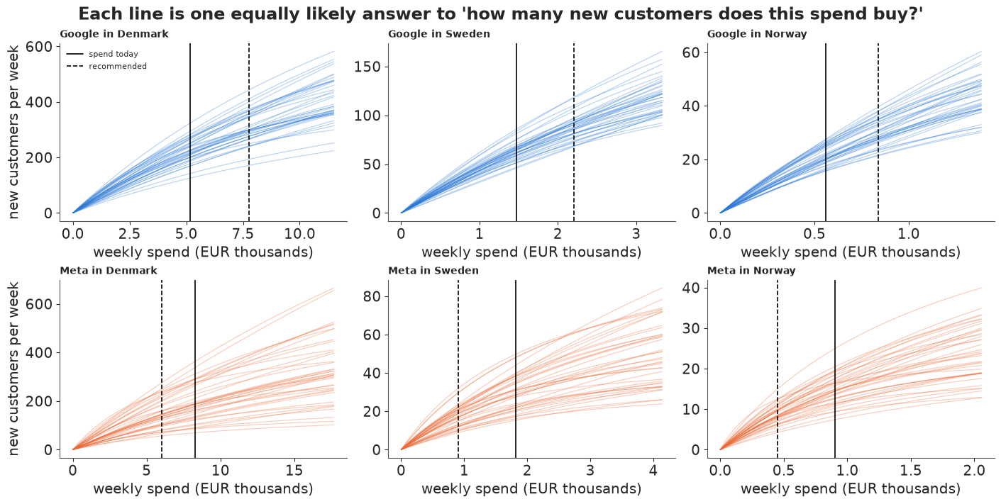
9.1 What does each extra euro buy? Forty equally likely response curves
A band suggests one true curve with fuzzy edges. Forty curves drawn from the posterior show what the model actually believes: a family of possible curves, each one consistent with the data. The marks show where each budget line sits now and where the recommended plan puts it.
n_spag = 40
spag = cur_part[rng.choice(len(cur_part), n_spag, replace=False)]
fig, axes = plt.subplots(2, 3, figsize=(14, 7))
spend_now_wk = BUDGET / LAST
for i, m in enumerate(MARKETS):
    for j, c in enumerate(CHANNELS):
        ax = axes[j, i]
        spend_axis = grid_mult * S_MEAN[i, j]
        for s_ in spag:
            ax.plot(spend_axis / 1000, s_[i, j], color=CH_COLOR[c], lw=0.8, alpha=0.35)
        ax.axvline(spend_now_wk[i, j] / 1000, color="k", lw=1.2, label="spend today")
        ax.axvline(plan_mean[i, j] * spend_now_wk[i, j] / 1000, color="k", lw=1.2, ls="--",
                   label="recommended")
        ax.set_title(f"{c} in {m}", loc="left", fontsize=10)
        ax.set_xlabel("weekly spend (EUR thousands)")
    axes[0, 0].legend(fontsize=8, loc="upper left")
axes[0, 0].set_ylabel("new customers per week")
axes[1, 0].set_ylabel("new customers per week")
fig.suptitle("Each line is one equally likely answer to 'how many new customers does this spend buy?'");
9.2 Twenty equally likely outcomes of the plan
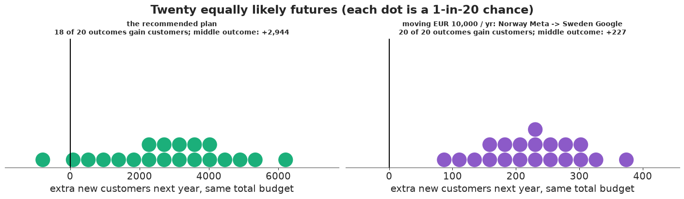
A quantile dotplot (Kay et al. 2016): twenty dots, each one a 5% chance, placed at the posterior quantiles. "How likely is it that the plan loses customers?" becomes "count the dots left of zero". Left: the full recommended plan. Right: a single, concrete move of 10,000 euros a year from the budget line with the most expensive marginal customer to the one with the cheapest.
def quantile_dotplot(ax, samples, n_dots=20, n_bins=22, color=BLUE, xlim=None, max_stack=8):
    """Wilkinson-style dotplot of the n_dots quantiles of `samples` (as in E16)."""
    qd = np.quantile(samples, (np.arange(n_dots) + 0.5) / n_dots)
    lo_, hi_ = xlim if xlim is not None else (qd.min(), qd.max())
    edges = np.linspace(lo_, hi_, n_bins + 1)
    width = edges[1] - edges[0]
    cols = np.clip(np.digitize(qd, edges) - 1, 0, n_bins - 1)
    heights = np.zeros(n_bins, int)
    for cix in cols:
        ax.add_patch(Ellipse((edges[cix] + width / 2, heights[cix] + 0.5), width * 0.92, 0.92, color=color))
        heights[cix] += 1
    ax.set(xlim=(lo_, hi_), ylim=(0, max_stack + 0.5), yticks=[])
    ax.set_aspect(width)
    sns.despine(ax=ax, left=True)
    return qd


med_mc = np.median(mcost_now, axis=0)
src, dst = np.unravel_index(med_mc.argmax(), med_mc.shape), np.unravel_index(med_mc.argmin(), med_mc.shape)
MOVE = 10_000.0
r_move = np.ones((M, C))
r_move[src] -= MOVE / BUDGET[src]
r_move[dst] += MOVE / BUDGET[dst]
g_plan, g_move = planner.gain(plan_mean), planner.gain(r_move)
move_label = f"{MARKETS[src[0]]} {CHANNELS[src[1]]} -> {MARKETS[dst[0]]} {CHANNELS[dst[1]]}"

fig, axes = plt.subplots(1, 2, figsize=(14, 3.8))
for ax, g, col, title in [(axes[0], g_plan, AQUA, "the recommended plan"),
                          (axes[1], g_move, PURPLE, f"moving EUR 10,000 / yr: {move_label}")]:
    span = max(abs(np.quantile(g, 0.01)), abs(np.quantile(g, 0.99))) * 1.1
    qd = quantile_dotplot(ax, g, color=col, xlim=(min(-0.15 * span, np.quantile(g, 0.01) * 1.1), span))
    ax.axvline(0, color="k", lw=1.5)
    n_neg = int((qd < 0).sum())
    ax.set_xlabel("extra new customers next year, same total budget")
    ax.set_title(f"{title}\n{20 - n_neg} of 20 outcomes gain customers; "
                 f"middle outcome: {np.median(g):+,.0f}", fontsize=10)
fig.suptitle("Twenty equally likely futures (each dot is a 1-in-20 chance)", y=1.04);
9.3 Where does the next 1,000 euros work hardest?
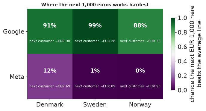
For each budget line, the chance that the next 1,000 euros there buys more new customers than the same 1,000 euros spread across the current plan (the budget-weighted average of all six lines). Green: a good place to add money; purple: a good place to take it from. The number underneath is the model's middle estimate of what the next new customer costs there.
next_1000 = 1000.0 / mcost_now  # customers per extra 1,000 EUR, (draws, m, c)
avg_1000 = (next_1000 * BUDGET).sum(axis=(1, 2)) / BUDGET.sum()
p_better = (next_1000 > avg_1000[:, None, None]).mean(axis=0)

fig, ax = plt.subplots(figsize=(7, 3.6))
im = ax.imshow(p_better.T, cmap="PRGn", vmin=0, vmax=1)
for i in range(M):
    for j in range(C):
        ax.text(i, j - 0.12, f"{100 * p_better[i, j]:.0f}%", ha="center", va="center", fontsize=14,
                color="white" if abs(p_better[i, j] - 0.5) > 0.35 else "k", weight="bold")
        ax.text(i, j + 0.22, f"next customer ~EUR {med_mc[i, j]:.0f}", ha="center", va="center", fontsize=8,
                color="white" if abs(p_better[i, j] - 0.5) > 0.35 else "k")
ax.set(xticks=range(M), xticklabels=MARKETS, yticks=range(C), yticklabels=CHANNELS)
ax.grid(False)
plt.colorbar(im, ax=ax, label="chance the next EUR 1,000 here\nbeats the average line", shrink=0.8)
ax.set_title("Where the next 1,000 euros works hardest", fontsize=11);
9.4 Small markets borrow strength
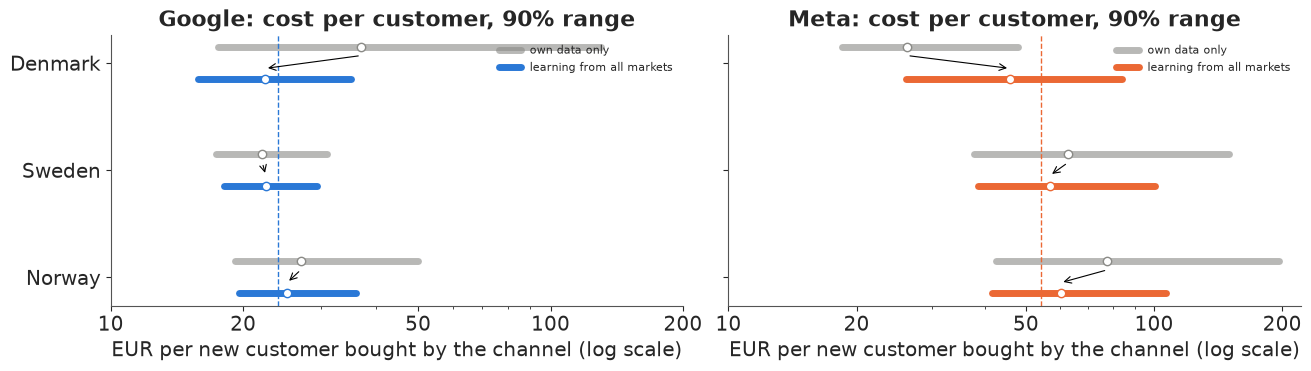
Why trust a number for Norway, where only about 60 new customers arrive a week? Because the model does not estimate Norway alone. Each line below is a 90% range for what a customer costs in euros: grey from the market's own data only, coloured from the model that also learns from the other two markets. The dashed line is the channel's average across markets.
qn, qp = q(idata_none, "cpc"), q(idata, "cpc")
mu_ch = np.exp(idata.posterior["mu_log_cpc"].median(("chain", "draw")).to_numpy())
fig, axes = plt.subplots(1, 2, figsize=(13, 3.6), sharey=True)
for j, (ax, c) in enumerate(zip(axes, CHANNELS)):
    for i, m in enumerate(MARKETS):
        y0 = M - 1 - i
        ax.plot([qn[0, i, j], qn[2, i, j]], [y0 + 0.15] * 2, color=GREY, lw=5, solid_capstyle="round",
                alpha=0.6, label="own data only" if i == 0 else None)
        ax.plot(qn[1, i, j], y0 + 0.15, "o", color="white", mec=GREY, ms=6)
        ax.plot([qp[0, i, j], qp[2, i, j]], [y0 - 0.15] * 2, color=CH_COLOR[c], lw=5,
                solid_capstyle="round", label="learning from all markets" if i == 0 else None)
        ax.plot(qp[1, i, j], y0 - 0.15, "o", color="white", mec=CH_COLOR[c], ms=6)
        ax.annotate("", xy=(qp[1, i, j], y0 - 0.05), xytext=(qn[1, i, j], y0 + 0.07),
                    arrowprops={"arrowstyle": "->", "color": "k", "lw": 0.8})
    ax.axvline(mu_ch[j], color=CH_COLOR[c], ls="--", lw=1)
    ax.set(xscale="log", xlabel="EUR per new customer bought by the channel (log scale)",
           title=f"{c}: cost per customer, 90% range")
    ax.set_xticks([10, 20, 50, 100, 200], labels=["10", "20", "50", "100", "200"])
    ax.legend(fontsize=8, loc="upper right")
axes[0].set(yticks=range(M), yticklabels=MARKETS[::-1]);
What each display is for, and what it says here:
- Forty response curves make "we are not sure" concrete without an interval in sight. In Denmark the curves fan out widely - the two channels there are hard to separate - while the Swedish and Norwegian Google curves are tight. The dashed marks show that the plan moves spend along the curves the data know, never past their ends.
- Twenty dots answer the question finance will actually ask - "could this lose us customers?" - by counting: 18 of 20 outcomes of the full plan gain, two do not; the small concrete move from Norwegian Meta to Swedish Google gains in all twenty.
- The heatmap replaces six intervals with one probability per budget line and the one number a marketer uses (what the next customer costs). Read it as "take from purple, add to green".
- Borrowing strength is the hierarchy explained without the word: each market's own range (grey) is pulled toward what the other markets say (coloured), most where its own data are weakest - Norway's Meta and Denmark's split.
All four should travel with the caveat of section 8: these are the model's odds, given that spend did not chase demand. Moving from "the model's odds" to "the world's odds" is what a geo experiment is for.
9.5 Export for the web page
The decision-relevant results go into one small JSON file (a few hundred draws, curves as quantiles on a grid, plain-English headlines), from which a page for non-technical readers can be built without re-running the model.
root = next(p for p in [Path.cwd(), *Path.cwd().parents] if (p / "pyproject.toml").exists())
cell = [f"{m}|{c}" for m in MARKETS for c in CHANNELS]
sub = rng.choice(len(g_plan), 300, replace=False)
qs = [0.05, 0.25, 0.5, 0.75, 0.95]
curve_q = np.quantile(cur_part, qs, axis=0)  # (q, m, c, grid)
export = {
    "id": "E33",
    "title": "Hierarchical multi-market MMM: where should next year's paid budget go?",
    "brand": "Scandinavian apparel brand (anonymised, Conjura open MMM data, CC BY 4.0)",
    "period": f"{weeks[0].date()} to {weeks[-1].date()} (81 weeks)",
    "currency": "EUR (fixed ECB 2023 average rates)",
    "markets": MARKETS, "channels": CHANNELS, "cells": cell,
    "current_plan_eur_per_year": dict(zip(cell, BUDGET.ravel().round(0).tolist())),
    "recommended_plan_eur_per_year": dict(zip(cell, (plan_mean * BUDGET).ravel().round(0).tolist())),
    "cautious_plan_eur_per_year": dict(zip(cell, (plan_safe * BUDGET).ravel().round(0).tolist())),
    "media_customers_now_per_year": {"median": float(np.median(planner.now)),
                                     "q05": float(np.quantile(planner.now, 0.05)),
                                     "q95": float(np.quantile(planner.now, 0.95))},
    "plan_gain": {"unit": "extra new customers next year",
                  "draws": g_plan[sub].round(0).astype(int).tolist(),
                  "median": float(np.median(g_plan)), "q05": float(np.quantile(g_plan, 0.05)),
                  "q95": float(np.quantile(g_plan, 0.95)), "p_beats_current": float((g_plan > 0).mean())},
    "move_example": {"from": f"{MARKETS[src[0]]}|{CHANNELS[src[1]]}", "to": f"{MARKETS[dst[0]]}|{CHANNELS[dst[1]]}",
                     "eur_per_year": MOVE, "draws": g_move[sub].round(0).astype(int).tolist(),
                     "median": float(np.median(g_move)), "p_positive": float((g_move > 0).mean())},
    "marginal_cost_eur": {"unit": "EUR per extra new customer at today's spend",
                          **{f"q{int(100 * qq):02d}": dict(zip(cell, np.quantile(mcost_now, qq, axis=0).ravel().round(1).tolist()))
                             for qq in qs},
                          "draws": {cl: v.round(1).tolist() for cl, v in
                                    zip(cell, mcost_now[sub[:200]].reshape(200, -1).T)}},
    "p_next_1000_beats_average": dict(zip(cell, p_better.ravel().round(3).tolist())),
    "response_curves": {"unit": "new customers per week at a sustained weekly spend",
                        "spend_eur_per_week": {cl: (grid_mult * S_MEAN.ravel()[n]).round(0).tolist()
                                               for n, cl in enumerate(cell)},
                        "spend_today_eur_per_week": dict(zip(cell, spend_now_wk.ravel().round(0).tolist())),
                        "quantiles": {f"q{int(100 * qq):02d}": {cl: curve_q[n_q].reshape(M * C, -1)[n].round(1).tolist()
                                                                 for n, cl in enumerate(cell)}
                                      for n_q, qq in enumerate(qs)}},
    "shrinkage_cost_per_customer_eur": {
        "own_data_only": {cl: qn[:, n // C, n % C].round(1).tolist() for n, cl in enumerate(cell)},
        "pooled": {cl: qp[:, n // C, n % C].round(1).tolist() for n, cl in enumerate(cell)},
        "channel_average": dict(zip(CHANNELS, mu_ch.round(1).tolist())), "quantiles": [0.05, 0.5, 0.95]},
    "prior_sensitivity": sens.reset_index().round(3).to_dict(orient="records"),
    "headlines": {},  # filled below
}
lo_c, hi_c = np.unravel_index(med_mc.argmin(), med_mc.shape), np.unravel_index(med_mc.argmax(), med_mc.shape)
i_no, j_me = MARKETS.index("Norway"), CHANNELS.index("Meta")
export["headlines"] = HEADLINES = {
    "plan_gain": (f"Re-splitting the same total budget across channels and markets most likely brings "
                  f"about {np.median(g_plan):,.0f} extra new customers next year (9 in 10 chance: "
                  f"{np.quantile(g_plan, 0.05):,.0f} to {np.quantile(g_plan, 0.95):,.0f}); the chance it "
                  f"beats today's plan is {(g_plan > 0).mean():.0%}."),
    "move_example": (f"Moving EUR 10,000 a year from {move_label.replace(' -> ', ' to ')} most likely "
                     f"adds about {np.median(g_move):,.0f} new customers; the chance it helps at all is "
                     + ("over 99%." if (g_move > 0).mean() > 0.99 else f"{(g_move > 0).mean():.0%}.")),
    "marginal_cost": (f"The next new customer is cheapest via {CHANNELS[lo_c[1]]} in {MARKETS[lo_c[0]]} "
                      f"(about EUR {med_mc[lo_c]:.0f}) and dearest via {CHANNELS[hi_c[1]]} in "
                      f"{MARKETS[hi_c[0]]} (about EUR {med_mc[hi_c]:.0f})."),
    "shrinkage": (f"On its own data, Norway's cost per Meta customer could be anywhere from EUR "
                  f"{qn[0, i_no, j_me]:.0f} to {qn[2, i_no, j_me]:.0f}; learning from Denmark and Sweden "
                  f"narrows that to EUR {qp[0, i_no, j_me]:.0f}-{qp[2, i_no, j_me]:.0f}."),
    "caveat": ("These are model estimates without any experiment. Google spend partly follows demand, "
               "which flatters Google in every model of this kind: test before moving large sums."),
}
out = root / ".scratch" / "artifact" / "E33.json"
out.parent.mkdir(parents=True, exist_ok=True)
out.write_text(json.dumps(export, separators=(",", ":")))
print(f"wrote {out.relative_to(root)} ({out.stat().st_size / 1024:.0f} KB)")
for v in HEADLINES.values():
    print("-", v)
wrote .scratch/artifact/E33.json (30 KB)
- Re-splitting the same total budget across channels and markets most likely brings about 2,944 extra new customers next year (9 in 10 chance: -392 to 5,778); the chance it beats today's plan is 92%.
- Moving EUR 10,000 a year from Norway Meta to Sweden Google most likely adds about 227 new customers; the chance it helps at all is over 99%.
- The next new customer is cheapest via Google in Sweden (about EUR 28) and dearest via Meta in Norway (about EUR 93).
- On its own data, Norway's cost per Meta customer could be anywhere from EUR 42 to 196; learning from Denmark and Sweden narrows that to EUR 42-107.
- These are model estimates without any experiment. Google spend partly follows demand, which flatters Google in every model of this kind: test before moving large sums.
The page export above keeps a few hundred draws. The interactive Lumen reports in reports/
use the full posterior instead: every chain and draw of the fitted parameters, plus the
quantities derived from them over all the draws they were computed on
(reports/posteriors/E33.nc, see reports/README.md).
from pymc_challenges.export import save_posterior

save_posterior("E33", idata, {
    "plan_gain": (("sample",), g_plan, {}, "new customers per year",
                  "extra new customers next year from the recommended budget split versus the current one (same total spend)"),
    "move_10k_norway_meta_to_sweden_google": (("sample",), g_move, {}, "new customers per year",
                                               "extra new customers from moving EUR 10,000 a year from Norway Meta to Sweden Google"),
    "marginal_cost_eur": (("sample", "market", "channel"), mcost_now, {"market": MARKETS, "channel": CHANNELS},
                          "EUR per new customer", "cost of one extra new customer at today's spend"),
    "customers_per_week": (("sample", "market", "channel", "spend_multiple"), cur_part,
                           {"market": MARKETS, "channel": CHANNELS, "spend_multiple": grid_mult}, "new customers per week",
                           "steady-state new customers per week at a sustained weekly spend (x: multiple of the cell's average weekly spend)"),
}, x_dims=("spend_multiple",));
wrote reports/posteriors/E33.nc: 22 parameters x 4000 draws; 4 derived quantities; 3.1 MB
What to take away
- An MMM is adstock + saturation + a baseline + a prior, and each piece is a few lines of PyMC. Building it yourself makes every assumption visible - including the ones that decide the answer.
- Parameterise in business units. Priors on cost per incremental customer can be checked against numbers a marketer knows (blended CAC), are exchangeable across markets, and put the prior on the quantity the data inform best: the level of the curve at current spend.
- Pool curves across markets. Small markets get usable curves; collinear markets get a sensible split. Centred and non-centred forms fail at opposite ends of the posterior; look at where the divergences are before choosing a fix.
- LOO will not tell you the attribution is right. Models with very different channel splits predict new customers almost equally well.
- Optimise on the posterior, then evaluate over it. Report the expected gain, its range, and P(new plan beats current); know that bounds, not curves, often set the size of the move; a risk-adjusted objective moves money where the evidence is strongest.
- Separate what the priors can change from what the assumptions can. A prior sensitivity that comes back clean is not a validation: endogenous spend biases every channel curve, and only an experiment (next section, item 1) can tell you by how much.
Try it yourself
- Add a lift test. Suppose the brand ran a two-week geo holdout that switched Meta off in
Norway and measured $\Delta$ fewer new customers with standard error $s$ (this dataset has
no such experiment, so do not invent one for a real report). The model's prediction of
that experiment is a deterministic function of the parameters: the media customers of
Norway-Meta summed over the test weeks (and the adstock tail after them), computed with
spend set to zero minus spend as observed. Add
pm.Normal("lift", mu=predicted_lift, sigma=s, observed=delta). This is how PyMC-Marketing and Meridian calibrate to experiments, and it pins down the level of the curve that section 8 showed is partly prior-driven. How much does one such test narrow the Norway Meta curve - and, through the hierarchy, the Denmark and Sweden Meta curves? - Split Google. Performance Max and paid search capture existing demand; video and shopping less so. Split Google into two channels, give each its own pooled curve, and see whether the recommended shift toward Google survives. Then add E32's copula control for the demand-chasing channel.
- Pool on a different scale. Replace the cost-per-customer parameterisation with
Meridian's alternative (a coefficient on spend scaled by market population or by the
market's median spend) and pool that instead. Which markets move, and does the decision
change? Pool the Hill slope too (free slope,
LogNormal(0, 0.3)): do S-shaped curves appear, and are they supported by LOO?