Designing a thermal gradient plate: Bayesian calibration and optimal placement of heaters, insulation and sensors for the 2-D heat equation

#The problem, in one paragraph

Many instruments need a surface held at a precise temperature gradient rather than a single temperature: gradient plates for testing seed germination or bacterial growth at many temperatures at once, gradient PCR blocks, directional solidification of alloys and crystals, thermophoresis cells. The engineer controls where heat goes in (heating elements), where it is kept in (insulation) and where it is measured (sensors that feed a controller). Heat does the rest by spreading through the plate and leaking to the room, according to the heat equation. The difficulty is that the plate's properties are only approximately known, and the room does not stay the same. Here we design such a plate: a 40 × 20 cm metal plate whose central working area must run from 30 °C at the left to 70 °C at the right, uniformly across its width, in a 20 °C room. We learn the plate's physics from a short calibration experiment, then choose heaters, insulation and sensors to hit the gradient in all plausible versions of the plate and the room, not just the most likely one.

#The plan

1. The heat equation on a plate, as a linear system
2. Calibration: learning the plate's physics
3. Where to put the heaters, and how hard to drive them
4. Insulation: passive robustness
5. Sensors and feedback: holding the gradient when the room changes
6. The final design

import logging
import time

import arviz as az
import matplotlib.pyplot as plt
import numpy as np
import pymc as pm
import pytensor.tensor as pt
from IPython.display import HTML
from matplotlib import animation
from matplotlib.patches import Rectangle
from scipy.optimize import lsq_linear

RANDOM_SEED = 51
rng = np.random.default_rng(RANDOM_SEED)
az.style.use("arviz-variat")
logging.getLogger("pymc").setLevel(logging.WARNING)
BLUE, ORANGE, AQUA, GREY, PURPLE, RED, INK = (
    "#2a78d6", "#eb6834", "#1baf7a", "#8a8a86", "#8c5ac8", "#c8384e", "#222222")
print(f"PyMC {pm.__version__}, ArviZ {az.__version__}")

PyMC 6.3.2, ArviZ 1.3.0

#1 · The heat equation on a plate, as a linear system

A thin plate of thickness $\delta$ and conductivity $k$ conducts heat in its plane and loses heat to the room through its two faces (heat-transfer coefficient $h$, W m⁻² K⁻¹) and its edges ($h_e$). Heaters add power density $q(x, y)$, of which a fraction $\eta$ reaches the plate. At steady state, with $u = T - T_{\text{room}}$,

$$k\,\delta\,\nabla^2 u \;-\; (h_{\text{front}} + h_{\text{back}}(x, y))\,u \;+\; \eta\,q \;=\; 0,$$

plus $-k\,\partial_n u = h_e\,u$ on the edges. We split the plate into 24 × 12 square cells of 1.67 cm and write the heat balance of each cell (a finite-volume discretisation): conduction to its four neighbours, loss through its faces and any edges, and the heater power it receives. The result is a linear system

$$A(\theta)\,u = \eta\,q, \qquad A(\theta) = -k\,\delta\,L + \mathrm{diag}\big(h\,(1 + m_{\text{back}})\,\Delta x^2 + h_e\,\delta\,\Delta x\,n_{\text{edge}}\big),$$

where $L$ is the graph Laplacian of the grid, $m_{\text{back}}$ is 1 on bare back face and 0.1 under insulation, and $n_{\text{edge}}$ counts a cell's outer edges. Two consequences shape the whole design:

• Superposition. $u$ is linear in the heater powers: $u = \sum_i p_i\,g_i(\theta)$, where $g_i$ is heater $i$'s influence map (the temperature rise per watt). Choosing powers is a linear least-squares problem.
• A heat-spreading length. Heat conducted in the plane competes with heat lost through the faces over a distance $\ell = \sqrt{k\delta / 2h}$, about 13 cm here. A single heater warms a region of about that size and no more, so a smooth gradient over 30 cm needs several heaters, each doing part of the job.

We take a brass-like plate: $\delta = 5$ mm, and "true" values $k = 60$ W m⁻¹ K⁻¹, $h = 9$, $h_e = 15$ W m⁻² K⁻¹, $\eta = 0.93$ (the truth is unknown to the designer).

LX, LY, NX, NY = 0.40, 0.20, 24, 12
DX = LX / NX
DELTA, T_ROOM = 0.005, 20.0
xc, yc = (np.arange(NX) + 0.5) * DX, (np.arange(NY) + 0.5) * DX
X, Y = np.meshgrid(xc, yc, indexing="xy")
N = NX * NY


def cell(i, j):
    return j * NX + i


LAP = np.zeros((N, N))
N_EDGE = np.zeros(N)
for j in range(NY):
    for i in range(NX):
        a = cell(i, j)
        for di, dj in [(1, 0), (-1, 0), (0, 1), (0, -1)]:
            if 0 <= i + di < NX and 0 <= j + dj < NY:
                LAP[a, a] -= 1
                LAP[a, cell(i + di, j + dj)] += 1
            else:
                N_EDGE[a] += 1


def operator(k, h, h_edge, back=None, h_factor=None):
    """A(theta): conduction + face loss (h_factor: spatial multiplier for drafts) + edge loss."""
    back = np.ones(N) if back is None else back
    hf = np.ones(N) if h_factor is None else h_factor
    return -k * DELTA * LAP + np.diag(h * hf * (1 + back) * DX**2 + h_edge * DELTA * DX * N_EDGE)


def influence(theta, sites, back=None, h_factor=None, eff=None):
    """Temperature rise (K) per watt for heaters at the given cells: (N, n_sites)."""
    q = np.zeros((N, len(sites)))
    q[sites, np.arange(len(sites))] = theta["eta"] * (1.0 if eff is None else eff)
    return np.linalg.solve(operator(theta["k"], theta["h"], theta["h_edge"], back, h_factor), q)


THETA_TRUE = dict(k=60.0, h=9.0, h_edge=15.0, eta=0.93)
WORK = ((X >= 0.05) & (X <= 0.35) & (Y >= 0.03) & (Y <= 0.17)).ravel()   # working area
T_TARGET = (30 + 40 * (X - 0.05) / 0.30).ravel()
ell = np.sqrt(THETA_TRUE["k"] * DELTA / (2 * THETA_TRUE["h"]))
print(f"heat-spreading length sqrt(k delta / 2h) = {100 * ell:.1f} cm")


def show_field(ax, field, title, vmin=20, vmax=75, cmap="inferno"):
    im = ax.imshow(field.reshape(NY, NX), origin="lower", extent=[0, 100 * LX, 0, 100 * LY],
                   vmin=vmin, vmax=vmax, cmap=cmap, aspect="equal")
    ax.add_patch(Rectangle((5, 3), 30, 14, fill=False, ec="white", lw=1, ls="--"))
    ax.set(title=title, xlabel="x (cm)", ylabel="y (cm)")
    return im


demo_site = [cell(12, 6)]
fig, axes = plt.subplots(1, 2, figsize=(12, 3.4))
im = show_field(axes[0], T_ROOM + 10 * influence(THETA_TRUE, demo_site)[:, 0], "One 10 W heater (true plate)")
fig.colorbar(im, ax=axes[0], label="°C")
im = show_field(axes[1], T_TARGET, "The target: 30 → 70 °C across the working area (dashed)")
fig.colorbar(im, ax=axes[1], label="°C");

heat-spreading length sqrt(k delta / 2h) = 12.9 cm

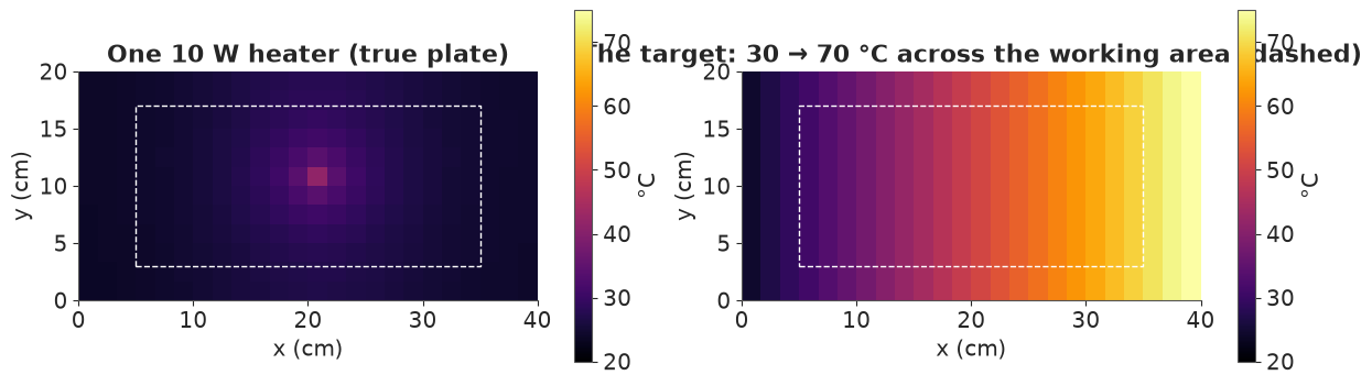
One 10 W heater warms a patch about 10-15 cm across by a few degrees: heat does not travel far before it leaks out of the faces. The target (right) is a ramp in $x$, flat in $y$, over the dashed working area; outside it the temperature is free.

#2 · Calibration: learning the plate's physics

The designer does not know $k$, $h$, $h_e$ or $\eta$ exactly. A calibration experiment: three runs, each with one 10 W test heater at a different place, and twelve thermocouples (±0.2 °C) glued at random positions. The model solves the discretised heat equation for each run inside PyMC (pt.linalg.solve on the 288 × 288 system, gradients included). Priors are order-of-magnitude: $k \sim$ LogNormal(log 50, 0.5) (brass or aluminium alloys), $h \sim$ LogNormal(log 10, 0.5) (natural convection plus radiation), $h_e \sim$ LogNormal(log 10, 0.7), $\eta \sim$ Beta(40, 4) (most of the electrical power reaches the plate).

cal_rng = np.random.default_rng(0)
test_sites = [cell(int(x / DX), int(y / DX)) for x, y in [(0.06, 0.10), (0.20, 0.05), (0.33, 0.14)]]
thermocouples = cal_rng.choice(N, 12, replace=False)
Q_test = np.zeros((3, N))
Q_test[np.arange(3), test_sites] = 10.0
T_cal_true = T_ROOM + np.linalg.solve(operator(THETA_TRUE["k"], THETA_TRUE["h"], THETA_TRUE["h_edge"]),
                                      THETA_TRUE["eta"] * Q_test.T).T[:, thermocouples]
T_cal = T_cal_true + 0.2 * cal_rng.standard_normal(T_cal_true.shape)

lap_t, edge_t = pt.as_tensor(LAP), pt.as_tensor(N_EDGE)
with pm.Model() as calibration:
    k = pm.LogNormal("k", np.log(50), 0.5)
    h = pm.LogNormal("h", np.log(10), 0.5)
    h_edge = pm.LogNormal("h_edge", np.log(10), 0.7)
    eta = pm.Beta("eta", 40, 4)
    sigma = pm.HalfNormal("sigma", 0.5)
    A = -k * DELTA * lap_t + pt.diag(2 * h * DX**2 + h_edge * DELTA * DX * edge_t)
    u = pt.linalg.solve(A, eta * Q_test.T).T                     # (runs, cells)
    pm.Normal("T_obs", T_ROOM + u[:, thermocouples], sigma, observed=T_cal)

t0 = time.time()
with calibration:
    idata = pm.sample(random_seed=RANDOM_SEED, progressbar=False, target_accept=0.9)
print(f"{time.time() - t0:.0f} s, {int(idata.sample_stats['diverging'].sum())} divergences")
summ = az.summary(idata, var_names=["k", "h", "h_edge", "eta", "sigma"], round_to=3)
summ["truth"] = [*THETA_TRUE.values(), 0.2]
print(summ[["mean", "sd", "eti89_lb", "eti89_ub", "ess_bulk", "r_hat", "truth"]])
post = idata.posterior.to_dataset().stack(sample=("chain", "draw"))
draw_idx = rng.choice(post.sizes["sample"], 200, replace=False)
THETA_DRAWS = [{v: float(post[v].values[i]) for v in ["k", "h", "h_edge", "eta"]} for i in draw_idx]
THETA_MEAN = {v: float(post[v].mean()) for v in ["k", "h", "h_edge", "eta"]}
print("correlations:", {f"{a}-{b}": round(float(np.corrcoef(post[a], post[b])[0, 1]), 2)
                        for a, b in [("k", "h"), ("k", "eta"), ("h", "eta")]})

18 s, 2 divergences
          mean     sd  eti89_lb  eti89_ub  ess_bulk  r_hat  truth
k       59.288  2.820    54.443    63.176   492.765  1.006  60.00
h        9.074  0.441     8.324     9.678   479.551  1.007   9.00
h_edge   6.774  3.511     2.355    13.295  1761.141  1.000  15.00
eta      0.912  0.042     0.839     0.967   453.637  1.007   0.93
sigma    0.189  0.023     0.156     0.230  2365.338  1.002   0.20
correlations: {'k-h': 0.91, 'k-eta': 0.96, 'h-eta': 0.95}

Three heaters and twelve thermocouples pin down the conductivity, the face coefficient and the heater efficiency to within about 4-5%, and their 89% intervals contain the true values. The three are strongly correlated (0.89-0.95, printout): thermocouples measure temperature rises, which depend on ratios like $\eta/k$ and $\eta/h$, so a less efficient heater on a less conductive, less leaky plate looks almost the same. The edge coefficient is barely learned: only a few thermocouples sit near an edge, and edges carry a small share of the heat. Its posterior is mostly prior, pulled towards the prior median of 10, and its 89% interval (about 2-13) misses the true value of 15. A weakly identified parameter plus a prior centred in the wrong place is how honest-looking intervals go wrong; the design will have to be robust to the edges, or a second experiment should put thermocouples near them.

#3 · Where to put the heaters, and how hard to drive them

Heater sites are chosen from a 12 × 6 lattice of 72 candidate positions. For a given set of sites, the powers minimise the expected squared error over the working area across posterior draws,

$$\min_{0 \le p_i \le p_{\max}}\; \mathbb{E}_{\theta \mid \text{calibration}}\, \big\lVert u_{\text{target}} - G(\theta)\,p \big\rVert^2_{\text{work}},$$

a constrained least-squares problem once the influence maps $G(\theta)$ of the candidate sites are stacked over 60 posterior draws (scipy.optimize.lsq_linear). The sites are added greedily: at each step, try every remaining candidate and keep the one that reduces the expected error most. Heaters may go anywhere in the frame around the working area (the 144 cells outside the dashed rectangle), not inside it: the working area is where the samples sit, and a heater there makes a local hot spot. (A first version of this notebook allowed heaters everywhere; the search put two inside the working area and the worst cells ended up 10 °C off target.) The heaters are rated at 20 W, but the nominal design may use at most 14 W per heater: headroom for the controller in section 5.

CANDIDATES = np.flatnonzero(~WORK)                                           # heaters stay in the frame
P_RATED, P_NOMINAL = 20.0, 14.0
design_draws = THETA_DRAWS[:60]
G_all = np.array([influence(th, CANDIDATES) for th in design_draws])        # (draws, N, 72)
G_plug = influence(THETA_MEAN, CANDIDATES)[None]                             # posterior mean only
u_target = (T_TARGET - T_ROOM)[WORK]


def fit_powers(G_stack, chosen, cap=P_NOMINAL):
    A = np.concatenate([g[WORK][:, chosen] for g in G_stack])
    b = np.tile(u_target, len(G_stack))
    return lsq_linear(A, b, bounds=(0, cap)).x


def expected_rms(G_stack, chosen, p):
    err = np.array([g[WORK][:, chosen] @ p - u_target for g in G_stack])
    return np.sqrt(np.mean(err**2))


def greedy_heaters(G_stack, n_heaters):
    chosen, path = [], []
    for _ in range(n_heaters):
        scores = [(expected_rms(G_stack, chosen + [c], fit_powers(G_stack, chosen + [c])), c)
                  for c in range(len(CANDIDATES)) if c not in chosen]
        best = min(scores)
        chosen.append(best[1])
        path.append(best[0])
    return chosen, path


t0 = time.time()
heaters, path = greedy_heaters(G_all, 8)
print(f"greedy search: {time.time() - t0:.0f} s; expected RMS error (°C) with 1..8 heaters:", np.round(path, 2))
N_HEAT = 6
sites = heaters[:N_HEAT]
p_design = fit_powers(G_all, sites)

# Alternatives for comparison, all evaluated over the SAME posterior draws
edge_rows = [c for c in range(len(CANDIDATES)) if CANDIDATES[c] // NX in (0, NY - 1)]
midline = [min(edge_rows, key=lambda c: abs(xc[CANDIDATES[c] % NX] - x0) + 10 * abs(CANDIDATES[c] // NX - row))
           for row in (0, NY - 1) for x0 in (0.15, 0.25, 0.35)]                 # 3 evenly along each long edge
p_midline = fit_powers(G_all, midline)
plug_sites, _ = greedy_heaters(G_plug, N_HEAT)
p_plug = fit_powers(G_plug, plug_sites)
eval_draws = np.array([influence(th, CANDIDATES) for th in THETA_DRAWS[60:200]])  # held-out draws
for name, s_, p_ in [("greedy, posterior", sites, p_design), ("evenly along the long edges", midline, p_midline),
                     ("greedy, plug-in (posterior mean)", plug_sites, p_plug)]:
    errs = np.array([np.sqrt(np.mean((g[WORK][:, s_] @ p_ - u_target) ** 2)) for g in eval_draws])
    print(f"{name:<34} powers {np.round(p_, 1)} (total {p_.sum():.0f} W); RMS error over 140 other "
          f"posterior draws: median {np.median(errs):.2f}, 90th pct {np.quantile(errs, 0.9):.2f} °C")

greedy search: 3 s; expected RMS error (°C) with 1..8 heaters: [23.09 13.92  5.75  2.21  1.7   1.43  1.39  1.35]

greedy, posterior                  powers [ 9.8  9.2  6.6  6.1  5.7 14. ] (total 51 W); RMS error over 140 other posterior draws: median 1.43, 90th pct 1.45 °C
evenly along the long edges        powers [ 1.7 10.3 14.   1.7 10.3 14. ] (total 52 W); RMS error over 140 other posterior draws: median 2.00, 90th pct 2.02 °C
greedy, plug-in (posterior mean)   powers [ 9.2  9.8  6.6  6.1  5.7 14. ] (total 51 W); RMS error over 140 other posterior draws: median 1.43, 90th pct 1.46 °C

Heater count. The expected error falls quickly with the first four heaters and flattens after six (printout); we use six. Placement matters: six heaters spaced evenly along the two long edges ("evenly" in the printout) give an RMS error of about 2.0 °C against 1.4 °C for the greedy layout, which puts most of its heat at the hot end, where the plate must be hottest, and adds smaller heaters along the edges halfway down.

Plug-in versus posterior design. Designing against the posterior-mean plate alone gives the same heater sites and nearly the same powers here, and the same error over 140 held-out posterior draws. That is a result, not a rule: the parameters the design depends on (conductivity, face loss, efficiency) are well determined as a group, and the poorly known edge coefficient matters little for the working area. The posterior still earns its keep: it says the error is 1.4-1.5 °C in almost every plausible plate, which the plug-in design alone cannot tell you, and it is what the controller in section 5 uses.

fig, axes = plt.subplots(1, 3, figsize=(15, 3.6))
for ax, (name, s_, p_) in zip(axes, [("Even edge heaters", midline, p_midline),
                                      ("Greedy heaters (posterior)", sites, p_design)]):
    field = T_ROOM + influence(THETA_TRUE, CANDIDATES[s_]) @ p_
    im = show_field(ax, field, f"{name}: the TRUE plate")
    for c, pw in zip(CANDIDATES[s_], p_):
        ax.plot(100 * xc[c % NX], 100 * yc[c // NX], "s", ms=4 + pw / 2, mfc="none", mec=AQUA, mew=1.5)
fig.colorbar(im, ax=axes[:2], label="°C", shrink=0.8)
ax = axes[2]
field = T_ROOM + influence(THETA_TRUE, CANDIDATES[sites]) @ p_design
work_x = X.ravel()[WORK]
ax.plot(100 * work_x, field[WORK], ".", ms=3, color=RED, label="greedy design, true plate")
field_mid = T_ROOM + influence(THETA_TRUE, CANDIDATES[midline]) @ p_midline
ax.plot(100 * work_x, field_mid[WORK], ".", ms=3, color=GREY, alpha=0.6, label="even edge heaters")
ax.plot([5, 35], [30, 70], color=INK, lw=1.5, label="target")
ax.set(xlabel="x (cm)", ylabel="°C", title="Every cell of the working area vs the target")
ax.legend(fontsize=8);

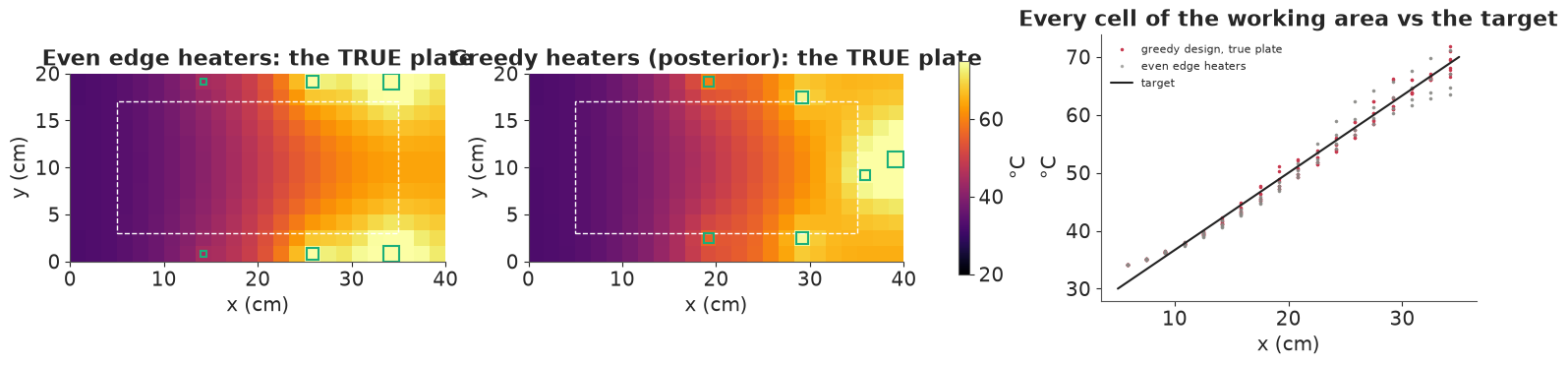
Squares mark the heaters (size = power). On the true plate the greedy design gives a ramp whose cells mostly sit within a degree or two of the target (right panel). The even edge heaters run too hot next to each heater and too cool between them along the middle. Neither design can reach the target at the cold end: the left column of the working area runs 2-4 °C too warm, because heat conducted from the right cannot be removed there - only a cooler (a heat sink at the left edge) could fix that.

#4 · Insulation: passive robustness

In operation the room changes. We model three kinds of disturbance, drawn independently for each scenario: the room temperature drifts ($\pm 2$ °C, sd), air currents change the face coefficient on the left and right halves of the plate independently (log-normal, sd 25%), and each heater's efficiency ages (sd 10%). Combined with the posterior of the plate's physics, this gives 120 plausible operating conditions.

Insulation acts before any controller: a pad on the back face cuts the loss there (to 10% of the bare value), so the plate depends less on drafts. We offer six vertical strips (6.7 cm wide) as candidates, choose up to two greedily by the expected error with the heater powers re-optimised for each insulation choice but without feedback, and record the power needed.

N_SCEN = 120
dist_rng = np.random.default_rng(5)
scen_theta = [THETA_DRAWS[i] for i in dist_rng.integers(len(THETA_DRAWS), size=N_SCEN)]
room_shift = dist_rng.normal(0, 2.0, N_SCEN)
draft_left, draft_right = np.exp(dist_rng.normal(0, 0.25, (2, N_SCEN)))
heater_age = np.exp(dist_rng.normal(0, 0.10, (N_SCEN, N_HEAT)))
LEFT = (X < LX / 2).ravel()
sensor_noise = 0.2 * dist_rng.standard_normal((N_SCEN, N))      # common random numbers
STRIPS = [(i0 * DX, (i0 + 4) * DX) for i0 in range(0, NX, 4)]


def back_mask(chosen_strips):
    m = np.ones(N)
    for s_ in chosen_strips:
        m[((X >= STRIPS[s_][0]) & (X < STRIPS[s_][1])).ravel()] = 0.1
    return m


def scenario_influences(back):
    return np.array([influence(th, CANDIDATES[sites], back, np.where(LEFT, dl, dr), age)
                     for th, dl, dr, age in zip(scen_theta, draft_left, draft_right, heater_age)])


def open_loop(back):
    """Re-optimise nominal powers for this insulation (no disturbances), then face the scenarios."""
    G_design = np.array([influence(th, CANDIDATES[sites], back) for th in design_draws[:30]])
    A = np.concatenate([g[WORK] for g in G_design])
    p = lsq_linear(A, np.tile(u_target, len(G_design)), bounds=(0, P_NOMINAL)).x
    G_s = scenario_influences(back)
    fields = T_ROOM + room_shift[:, None] + G_s @ p
    return p, G_s, fields


def rms_work(fields):
    return float(np.sqrt(np.mean((fields[:, WORK] - T_TARGET[WORK]) ** 2)))


t0 = time.time()
insulation_results = {}
chosen_strips = []
p_bare, G_bare, f_bare = open_loop(back_mask([]))
insulation_results["none"] = (rms_work(f_bare), p_bare.sum())
for _ in range(2):
    trials = []
    for s_ in range(len(STRIPS)):
        if s_ in chosen_strips:
            continue
        p_, _, f_ = open_loop(back_mask(chosen_strips + [s_]))
        trials.append((rms_work(f_), p_.sum(), s_))
    best = min(trials)
    chosen_strips.append(best[2])
    insulation_results[str([f"{100 * STRIPS[s][0]:.0f}-{100 * STRIPS[s][1]:.0f} cm" for s in chosen_strips])] = best[:2]
print(f"({time.time() - t0:.0f} s)")
for name, (e, pw) in insulation_results.items():
    print(f"insulation {name:<30} open-loop RMS error under disturbances {e:.2f} °C, nominal power {pw:.0f} W")

(1 s)
insulation none                           open-loop RMS error under disturbances 7.15 °C, nominal power 51 W
insulation ['27-33 cm']                   open-loop RMS error under disturbances 6.87 °C, nominal power 46 W
insulation ['27-33 cm', '33-40 cm']       open-loop RMS error under disturbances 6.55 °C, nominal power 40 W

Without feedback the disturbances dominate: a perfectly tuned open-loop plate is about 7 °C RMS off target, mostly because the room temperature shifts the whole plate and drafts change how much heat each region loses. The greedy choice insulates the hot end (the strips from 27 to 40 cm), where the plate is hottest above the room and loses most heat. That saves about a fifth of the heater power (51 → 40 W) and makes that end less sensitive to drafts, reducing the open-loop error a little (7.2 → 6.6 °C). Insulation cannot follow a room that is warmer or colder than planned: that is the job of sensors and feedback.

#5 · Sensors and feedback: holding the gradient when the room changes

A controller reads a few thermocouples and resets the heater powers. Ours is a Bayesian certainty-equivalence controller:

1. Estimate the disturbances $d$ = (room shift, log draft left, log draft right, log age of each heater) from the sensor readings with a linear-Gaussian update: prior $d \sim N(0, \Sigma_d)$ with the scales above, sensitivities $J = \partial T_{\text{sensors}}/\partial d$ from the posterior-mean model, and a noise covariance that includes both the ±0.2 °C sensor noise and the posterior uncertainty of the plate's physics at the sensor positions.
2. Re-optimise the heater powers for the model with the estimated disturbances, now allowed up to the full 20 W rating.

Then evaluate the true field in each scenario. The sensor positions are chosen greedily from 72 candidate positions by the Monte Carlo closed-loop error, and compared with: five sensors evenly spaced on the midline, sensors on (next to) the heaters, and an oracle that knows each scenario's disturbances and physics exactly (the best any sensor layout could do with these heaters).

BACK = back_mask(chosen_strips)
p_nom, G_scen, fields_open = open_loop(BACK)
n_d = 3 + N_HEAT
prior_sd = np.r_[2.0, 0.25, 0.25, 0.1 * np.ones(N_HEAT)]


def model_field(p, d):
    G = influence(THETA_MEAN, CANDIDATES[sites], BACK, np.where(LEFT, np.exp(d[1]), np.exp(d[2])), np.exp(d[3:]))
    return T_ROOM + d[0] + G @ p


f_nominal = model_field(p_nom, np.zeros(n_d))
J = np.stack([(model_field(p_nom, e * 1e-4) - model_field(p_nom, -e * 1e-4)) / 2e-4 for e in np.eye(n_d)], axis=1)
physics_spread = np.array([T_ROOM + influence(th, CANDIDATES[sites], BACK) @ p_nom for th in THETA_DRAWS])
C_physics = np.cov(physics_spread.T)


def closed_loop(sensors):
    s_ = list(sensors)
    Js = J[s_]
    R = C_physics[np.ix_(s_, s_)] + 0.2**2 * np.eye(len(s_))
    C0 = np.diag(prior_sd**2)
    gain = C0 @ Js.T @ np.linalg.inv(Js @ C0 @ Js.T + R)
    d_hat = (fields_open[:, s_] + sensor_noise[:, s_] - f_nominal[s_]) @ gain.T
    out = np.empty_like(fields_open)
    for s in range(N_SCEN):
        G_model = influence(THETA_MEAN, CANDIDATES[sites], BACK,
                            np.where(LEFT, np.exp(d_hat[s, 1]), np.exp(d_hat[s, 2])), np.exp(d_hat[s, 3:]))
        p = lsq_linear(G_model[WORK], u_target - d_hat[s, 0], bounds=(0, P_RATED)).x
        out[s] = T_ROOM + room_shift[s] + G_scen[s] @ p
    return out


oracle = np.array([T_ROOM + room_shift[s] + G_scen[s] @ lsq_linear(G_scen[s][WORK], u_target - room_shift[s],
                                                                    bounds=(0, P_RATED)).x for s in range(N_SCEN)])
t0 = time.time()
SENSOR_CANDIDATES = np.array([cell(i, j) for j in range(0, NY, 2) for i in range(0, NX, 2)])
chosen_sensors, sensor_path = [], []
for _ in range(5):
    best = min((rms_work(closed_loop(chosen_sensors + [c])), c) for c in SENSOR_CANDIDATES if c not in chosen_sensors)
    chosen_sensors.append(best[1])
    sensor_path.append(best[0])
print(f"greedy sensor search: {time.time() - t0:.0f} s")
layouts = {"greedy": chosen_sensors,
           "even, midline": [cell(i, 6) for i in (2, 7, 12, 17, 21)],
           "on the heaters": list(CANDIDATES[sites][:5])}
results = {"open loop (no sensors)": fields_open}
results.update({f"{k} (5 sensors)": closed_loop(v) for k, v in layouts.items()})
results["oracle"] = oracle
print("greedy RMS with 1..5 sensors:", np.round(sensor_path, 2))
for name, f in results.items():
    per = np.sqrt(np.mean((f[:, WORK] - T_TARGET[WORK]) ** 2, axis=1))
    print(f"{name:<28} RMS {rms_work(f):.2f} °C; worst cell error, 90th pct over scenarios "
          f"{np.quantile(np.abs(f[:, WORK] - T_TARGET[WORK]).max(1), 0.9):.1f} °C; "
          f"scenarios with RMS > 2.5 °C: {np.mean(per > 2.5):.0%}")

greedy sensor search: 14 s
greedy RMS with 1..5 sensors: [2.22 1.78 1.74 1.73 1.71]
open loop (no sensors)       RMS 6.55 °C; worst cell error, 90th pct over scenarios 15.6 °C; scenarios with RMS > 2.5 °C: 78%
greedy (5 sensors)           RMS 1.71 °C; worst cell error, 90th pct over scenarios 5.6 °C; scenarios with RMS > 2.5 °C: 5%
even, midline (5 sensors)    RMS 1.76 °C; worst cell error, 90th pct over scenarios 5.8 °C; scenarios with RMS > 2.5 °C: 6%
on the heaters (5 sensors)   RMS 1.84 °C; worst cell error, 90th pct over scenarios 5.2 °C; scenarios with RMS > 2.5 °C: 7%
oracle                       RMS 1.50 °C; worst cell error, 90th pct over scenarios 5.5 °C; scenarios with RMS > 2.5 °C: 0%

fig, axes = plt.subplots(1, 2, figsize=(13, 4))
ax = axes[0]
names = list(results)
per_scen = [np.sqrt(np.mean((results[n][:, WORK] - T_TARGET[WORK]) ** 2, axis=1)) for n in names]
ax.boxplot(per_scen, orientation="horizontal", tick_labels=names, showfliers=False)
ax.set(xlabel="RMS error over the working area (°C), 120 operating scenarios", xscale="log",
       title="Holding the gradient under disturbances")
ax = axes[1]
ax.plot(range(1, 6), sensor_path, "o-", color=RED, label="greedy placement")
ax.axhline(rms_work(oracle), color=AQUA, ls="--", label="oracle")
ax.axhline(rms_work(results["even, midline (5 sensors)"]), color=GREY, ls=":", label="5 even sensors")
ax.set(xlabel="number of sensors", ylabel="RMS error (°C)", title="Value of each extra sensor")
ax.legend(fontsize=8);

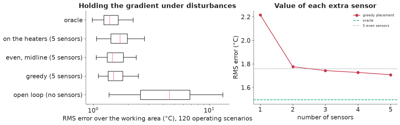
Feedback is the big step: from about 6.6 °C of open-loop error to 1.7 °C with five thermocouples, and the share of operating scenarios worse than 2.5 °C falls from about 80% to 5%. The first two sensors do almost all of it (right panel: 2.2 °C with one, 1.8 °C with two, then small gains), because the dominant disturbances - the room shift and the two drafts - are low-dimensional and a couple of well-placed readings pin them down.

Where the sensors go matters only modestly here: the greedy layout (1.71 °C) edges out five sensors spread evenly along the midline (1.76 °C), and sensors placed on the heaters are the worst of the three (1.84 °C). A sensor at a heater mostly measures that heater's own neighbourhood, which mixes its ageing with the local draft, and it says less about the working area. The greedy layout spreads its sensors over the working area and the hot end. The oracle, which knows every disturbance exactly, reaches 1.50 °C: the floor set by the heater layout itself. Better sensing can close at most the last 0.2 °C; beyond that, only better heaters (or a cooler at the cold end) help.

#6 · The final design

final = results["greedy (5 sensors)"]
fig, axes = plt.subplots(1, 2, figsize=(14, 4))
ax = axes[0]
im = show_field(ax, np.median(final, axis=0), "Median controlled field over 120 scenarios")
for s_ in chosen_strips:
    ax.add_patch(Rectangle((100 * STRIPS[s_][0], 0), 100 * (STRIPS[s_][1] - STRIPS[s_][0]), 100 * LY,
                           fill=True, fc="white", alpha=0.15, ec="white", lw=0.8, hatch="//"))
for c, pw in zip(CANDIDATES[sites], p_nom):
    ax.plot(100 * xc[c % NX], 100 * yc[c // NX], "s", ms=5 + pw / 2, mfc="none", mec=AQUA, mew=1.8)
for c in chosen_sensors:
    ax.plot(100 * xc[c % NX], 100 * yc[c // NX], "o", ms=6, mfc=BLUE, mec="white")
fig.colorbar(im, ax=ax, label="°C")
ax = axes[1]
err_q = np.quantile(np.abs(final - T_TARGET), 0.9, axis=0)
err_q[~WORK] = np.nan
im = ax.imshow(err_q.reshape(NY, NX), origin="lower", extent=[0, 100 * LX, 0, 100 * LY], cmap="viridis")
ax.set(title="90th-percentile |error| in the working area (°C)", xlabel="x (cm)", ylabel="y (cm)")
fig.colorbar(im, ax=ax, label="°C")
print(f"final design: {N_HEAT} heaters (nominal powers {np.round(p_nom, 1)} W, total {p_nom.sum():.0f} W), "
      f"insulation strips {[f'{100 * STRIPS[s][0]:.0f}-{100 * STRIPS[s][1]:.0f} cm' for s in chosen_strips]}, "
      f"sensors at (cm) {[(round(100 * xc[c % NX], 1), round(100 * yc[c // NX], 1)) for c in chosen_sensors]}");

final design: 6 heaters (nominal powers [ 7.2  6.1  2.1  6.3  5.8 12.4] W, total 40 W), insulation strips ['27-33 cm', '33-40 cm'], sensors at (cm) [(np.float64(24.2), np.float64(7.5)), (np.float64(17.5), np.float64(7.5)), (np.float64(37.5), np.float64(4.2)), (np.float64(20.8), np.float64(4.2)), (np.float64(20.8), np.float64(17.5))]

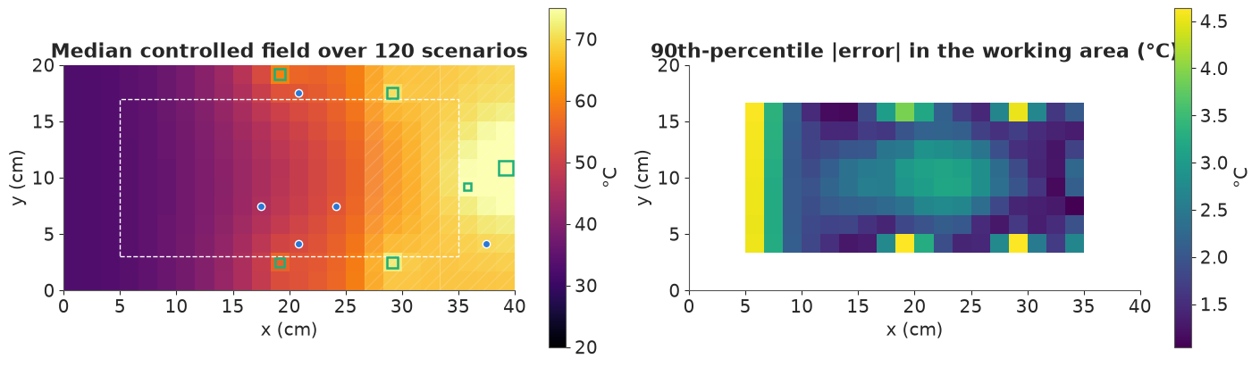
The final design: heater squares (size = nominal power), hatched back-face insulation, blue sensor dots. The error map shows where the design is weakest across the operating scenarios: the cold end of the working area (the left column, which runs warm because nothing removes heat there) and the cells next to the frame heaters at the top and bottom edges, which run hot. That points at the next improvements: a heat sink or cooled bar at the left edge, heaters spread over longer strips instead of small patches, and edge insulation to remove the least-known heat loss.

#Switching it on: how long until the gradient is ready?

Everything so far was steady state. A user also cares how long the plate takes to reach the gradient after it is switched on. That needs one more property, the plate's heat capacity per unit area, $\rho c\,\delta$ (brass: $\rho c \approx 3.2$ MJ m⁻³ K⁻¹, so 16 kJ m⁻² K⁻¹ at 5 mm). The transient heat equation on the same grid is $C\,\dot u = -A\,u + \eta\,q$ with $C = \rho c\,\delta\,\Delta x^2$ per cell. $A$ is symmetric, so one eigh gives the exact solution at any time, $u(t) = u_\infty - V e^{-\Lambda t / C} V^\top u_\infty$, with $u_\infty$ the steady field. The slowest mode, about $\rho c\,\delta / 2h \approx 15$ minutes, sets the time scale. The animation shows the true plate with the final design at its nominal powers, starting at room temperature; the lower panel is the profile along the centre line against the target.

RHO_C = 3.2e6                                                   # J m^-3 K^-1 (brass)
C_CELL = RHO_C * DELTA * DX**2


def warm_up(theta, times):
    """Exact transient temperatures (times, cells) from room temperature, final design, nominal powers."""
    A = operator(theta["k"], theta["h"], theta["h_edge"], BACK)
    q = np.zeros(N)
    q[CANDIDATES[sites]] = theta["eta"] * p_nom
    lam_w, V_w = np.linalg.eigh(A)
    u_inf = V_w @ ((V_w.T @ q) / lam_w)
    return T_ROOM + u_inf[None, :] - (np.exp(-lam_w[None, :] * times[:, None] / C_CELL)
                                      * (V_w.T @ u_inf)[None, :]) @ V_w.T


def ready_time(theta, tol=0.5):
    """Minutes until every working-area cell is within tol of its own steady temperature."""
    t_ = np.linspace(0, 3 * 3600, 721)
    T_ = warm_up(theta, t_)
    gap = np.abs(T_[:, WORK] - T_[-1, WORK]).max(axis=1)
    return t_[np.argmax(gap < tol)] / 60


t_anim = np.linspace(0, 60 * 60, 41)
T_anim = warm_up(THETA_TRUE, t_anim)
ready = np.array([ready_time(th) for th in THETA_DRAWS[:200]])
print(f"slowest time constant (true plate): {C_CELL / np.linalg.eigvalsh(operator(THETA_TRUE['k'], THETA_TRUE['h'], THETA_TRUE['h_edge'], BACK)).min() / 60:.1f} min")
print(f"time until the working area is within 0.5 C of steady state: true plate {ready_time(THETA_TRUE):.0f} min; "
      f"posterior median {np.median(ready):.0f} min (90%: {np.quantile(ready, 0.05):.0f}-{np.quantile(ready, 0.95):.0f})")

row = NY // 2
fig = plt.figure(figsize=(9, 6.5), dpi=72)
ax_f, ax_p = fig.subplots(2, 1, height_ratios=[1.3, 1])
im = show_field(ax_f, T_anim[0], "")
fig.colorbar(im, ax=ax_f, label="°C")
(prof_line,) = ax_p.plot(100 * xc, T_anim[0].reshape(NY, NX)[row], color=RED, lw=2, label="plate, centre line")
ax_p.plot(100 * xc, T_anim[-1].reshape(NY, NX)[row], ":", color=GREY, label="after 60 min")
ax_p.plot(100 * xc[(xc >= 0.05) & (xc <= 0.35)], T_TARGET.reshape(NY, NX)[row][(xc >= 0.05) & (xc <= 0.35)],
          "--", color=INK, label="target")
ax_p.set(xlabel="x (cm)", ylabel="°C", ylim=(15, 80))
ax_p.legend(fontsize=8, loc="upper left")
plt.close(fig)


def update(i):
    im.set_data(T_anim[i].reshape(NY, NX))
    ax_f.set_title(f"{t_anim[i] / 60:.1f} min after switching on")
    prof_line.set_ydata(T_anim[i].reshape(NY, NX)[row])
    return im, prof_line


anim = animation.FuncAnimation(fig, update, frames=len(t_anim), interval=150)
HTML(anim.to_jshtml(default_mode="once"))

slowest time constant (true plate): 16.8 min
time until the working area is within 0.5 C of steady state: true plate 74 min; posterior median 76 min (90%: 72-85)

The hot right end comes up first, because that is where most of the power goes in; the cool left end, fed only by conduction and the edge heaters, lags. The slowest mode has a time constant of about 17 minutes, but "ready" means every working-area cell within 0.5 °C of its final value, which takes several time constants: 74 minutes for the true plate (at 60 minutes, the end of the animation, the profile is still a degree short). Over the calibration posterior the answer is 76 minutes (90%: 72-85). That spread comes only from $k$, $h$ and $h_e$; the heat capacity was taken as known, and an error in it would scale every time proportionally. A faster start-up is a control problem the steady design does not solve: drive the heaters above their nominal powers for the first minutes (the headroom of section 5), then settle.

#Summary

• The 2-D heat equation becomes a linear system after a finite-volume discretisation, and the field is linear in heater powers: every design question reduces to influence maps and constrained least squares (section 1).
• Calibrate before designing. A small experiment fixes conductivity, face losses and heater efficiency as a group; the edge loss stays uncertain, and its interval even misses the truth (section 2).
• Design against the posterior: heater sites and powers chosen by expected error over plausible plates, with heaters kept out of the working area. Here the plug-in design happens to coincide, but only the posterior tells you how good the design is (section 3).
• Insulation is passive: a fifth less power and a little less sensitivity to drafts, but no answer to a changing room (section 4).
• Feedback with two to five sensors takes the error from about 7 °C to within 0.2 °C of the oracle; sensors on the heaters are the weakest choice. Leave power headroom so the controller can act. Some errors (the cold end) no controller of heaters alone can remove (sections 5-6).

#Try it yourself

1. Insulate the edges. Add edge insulation as a design option (multiply $h_e$ by 0.1 on chosen edges). Does it remove the corner errors of section 6, and does it make the design less sensitive to the poorly known edge coefficient?
2. Design the calibration. Choose the twelve calibration thermocouple positions (instead of random ones) to minimise the posterior variance of the design's error, not of the parameters. Where do they go, and how much does the final closed-loop error improve?
3. Transient control. Add heat capacity ($\rho c\,\delta\,\partial_t u$ on the left of the heat equation), step the room temperature at $t = 0$, and run the controller of section 5 every minute with an explicit time-stepping of the plate. How long does the gradient take to recover, and does the greedy sensor layout still win when the controller must act before steady state?