The setting
Two paint samples match perfectly in the shop. At home, under the kitchen's warm LEDs, one is visibly pinker than the other. Nothing is wrong with the paints or with your eyes: they are metamers, surfaces with different reflectance spectra that happen to produce the same three cone responses under one light, and not under another.
It follows from counting. A reflectance spectrum is a curve: here 41 numbers, one every 10 nm from 380 to 780 nm. A colour measurement (a colorimeter's CIELAB, or the eye's three cone signals) is 3 numbers. So "which spectrum has this colour?" has a 38-dimensional family of answers, and the colour of the same surface under a different light depends on where in that family the surface is.
That makes it a natural Bayesian problem:
- the likelihood says which spectra reproduce the measured colour (and it is flat along 38 directions);
- the prior says which spectra real surfaces have - and does almost all the work;
- the posterior is the set of plausible metamers, and its most useful summary is a prediction: the colour under the gallery's LEDs, with honest uncertainty.
We learn the prior from real measured surfaces (the Munsell chips), invert colours of chips that were held out, and check the predictions against their measured spectra.
| part | question | tool |
|---|---|---|
| A | What are the data, and how does a spectrum become a colour? | CIE observer, illuminants, CIELAB, CIEDE2000 |
| B | What can the observer not see? | null space, metameric blacks, metamer-mismatch bodies by linear programming |
| C | Which spectra are plausible? | three priors on logit-reflectance; held-out density; a closed-form preview |
| D | What does one colour say about the spectrum? | batched inversion in PyMC; spaghetti, swatch fans, mismatch clouds |
| E | Is the posterior honest? | coverage and PIT on held-out chips; where it is confident |
| F | One light or two? | a second measurement under incandescent light |
| G | Which paint recipe should we use? | expected ΔE00 under uncertain gallery lighting; value of information |
| H | An animation | walking through the metamers, physically possible vs plausible |
import io
import logging
import time
import warnings
from itertools import combinations

import arviz as az
import matplotlib.pyplot as plt
import numpy as np
import pandas as pd
import pymc as pm
import pytensor.tensor as pt
from IPython.display import HTML, Image, display
from matplotlib import animation
from matplotlib.patches import Ellipse, Patch
from scipy.optimize import linprog, minimize
from scipy.spatial import ConvexHull
from scipy.stats import beta as beta_dist

from pymc_challenges import data

RANDOM_SEED = 76
rng = np.random.default_rng(RANDOM_SEED)
az.style.use("arviz-variat")
logging.getLogger("pymc").setLevel(logging.WARNING)
warnings.filterwarnings("ignore", category=RuntimeWarning, module="arviz")
pd.set_option("display.width", 170)
pd.set_option("display.max_columns", 20)


def show_jpeg(fig, quality=85):
    """Swatch-heavy and many-coloured figures are far smaller as JPEG than PNG."""
    buf = io.BytesIO()
    fig.savefig(buf, format="jpeg", dpi=90, pil_kwargs={"quality": quality})
    plt.close(fig)
    display(Image(buf.getvalue()))
A. The data, and how a spectrum becomes a colour
The Munsell Book of Color is a physical atlas of painted chips arranged by hue (10 families, R, YR, Y, ..., RP, each at 2.5, 5, 7.5 and 10), value (lightness, 2.5 to 9) and chroma (colourfulness, 1 to 14). The University of Kuopio measured the reflectance spectrum of every chip of the matte edition, 1,269 of them: the fraction of light reflected at each wavelength. Our file keeps 10 nm steps (each value the mean of the 1 nm readings within ±4 nm).
The Zenodo record that mirrors the database gives its licence as "not specified". This repository keeps a derived 10 nm copy for teaching, with attribution to the database; anyone redistributing it further should check the terms with the database's owners.
data.describe("munsell_matt")
mun = data.load("munsell_matt")
data.describe("cie_illuminants_e76")
ill = data.load("cie_illuminants_e76").set_index("wavelength")
cie = data.load("cie1964_d65").set_index("wavelength")

WL = np.arange(380, 781, 10)                      # 41 wavelengths
R_ALL = mun[[f"r{w}" for w in WL]].to_numpy()
print(mun[["chip", "hue_family", "value", "chroma"]].sample(4, random_state=1).to_string(index=False))
print(f"{len(mun)} chips x {len(WL)} wavelengths; reflectance {R_ALL.min():.3f} to {R_ALL.max():.3f}")
munsell_matt: Reflectance spectra of the 1,269 chips of the Munsell Book of Color, Matte Finish Collection (1976), measured on a Perkin-Elmer Lambda 9 at 1 nm. One row per chip: chip (e.g. '2.5R 9/2'), hue, hue_family (R, YR, Y, GY, G, BG, B, PB, P, RP), value, chroma, r380 ... r780 (reflectance 0-1 at 10 nm, the mean of the 1 nm readings within +-4 nm).
  source: Munsell Colors Matt (spectrophotometer measured), University of Kuopio / University of Eastern Finland spectral color research database (Hauta-Kasari, n.d.; measured by J. Hiltunen), mirrored on Zenodo 3269912 by the colour-science project. Licence field on Zenodo: 'not specified'; cite the database. BUILT by tools/build_e76_metamers.py (10 nm means of the 1 nm data) - keep the cached file.
  url:    https://zenodo.org/records/3269912
cie_illuminants_e76: wavelength (380-780 nm, 5 nm) and relative spectral power of A (incandescent, 2856 K), FL2 (cool-white fluorescent), FL11 (narrow-band triphosphor fluorescent), LED_B2 and LED_B4 (phosphor-converted white LEDs).
  source: CIE illuminants (CIE 15:2004 tables, CIE 015:2018) as distributed with colour-science; A computed from Planck's law (CIE formula, checked against the table to 4e-6). Assembled by tools/build_e76_metamers.py.
  url:    https://raw.githubusercontent.com/colour-science/colour/develop/colour/colorimetry/datasets/illuminants/sds.py
    chip hue_family  value  chroma
10PB 7/8         PB    7.0       8
5YR 6/12         YR    6.0      12
7.5G 5/2          G    5.0       2
 10Y 8/2          Y    8.0       2
1269 chips x 41 wavelengths; reflectance 0.031 to 0.839The observer, the light and CIELAB
As in E74: the tristimulus values of a surface with reflectance $R(\lambda)$ under a light with power $S(\lambda)$ are sums of $R\,S\,\bar x$ (and $\bar y$, $\bar z$) over wavelength, with the CIE 1964 colour-matching functions, normalised so that a perfect white gives $X = Y = Z = 1$. CIELAB is then a fixed cube-root transform. Normalising by the white of the light in use is CIELAB's built-in (and crude) model of adaptation: a viewer who has adjusted to warm light sees a white wall as white. So "the colour under A" below means the colour a viewer adapted to A sees, and a swatch "rendered under A" is that colour shown on your (daylight-white) screen.
One detail matters here. The reflectances are known at 10 nm steps, but the lights are not smooth: the fluorescent FL11 concentrates its power in narrow mercury and phosphor lines. Sampling the light at the same 10 nm points throws most of a line away or doubles it. The right weights integrate the fine (1 nm) light x colour-matching functions against the linear interpolation of $R$ between the 10 nm nodes (a "hat" function per node) - the idea behind the ASTM E308 weighting tables. The table below compares the two for all 1,269 chips.
L1 = np.arange(380, 781)                                      # 1 nm grid
CMF = cie.loc[L1, ["xbar", "ybar", "zbar"]].to_numpy()
HAT = np.maximum(0, 1 - np.abs(L1[:, None] - WL[None]) / 10)  # 1 nm x node: linear interpolation
LIGHT_NAMES = {"D65": "daylight (D65)", "A": "incandescent (A)", "FL11": "fluorescent (FL11)",
               "LED_B2": "warm LED (LED-B2)"}
LIGHTS = list(LIGHT_NAMES)


def light_spd(name):
    """Relative power on the 1 nm grid (5 nm tables interpolated linearly)."""
    if name == "D65":
        return cie.loc[L1, "d65"].to_numpy()
    return np.interp(L1, ill.index, ill[name])


def observer(s):
    """41 x 3 weights: reflectance at the 10 nm nodes @ W -> XYZ relative to the light's white."""
    Wm = HAT.T @ (s[:, None] * CMF)
    return Wm / Wm.sum(0)


W = {k: observer(light_spd(k)) for k in LIGHTS}
D65_WHITE_2DEG = np.array([0.95047, 1.0, 1.08883])
M_SRGB = np.array([[0.4124, 0.3576, 0.1805], [0.2126, 0.7152, 0.0722], [0.0193, 0.1192, 0.9505]])


def xyz_to_lab(XYZ):
    d = 6 / 29
    f = np.where(XYZ > d**3, np.cbrt(np.maximum(XYZ, 1e-12)), XYZ / (3 * d**2) + 4 / 29)
    return np.stack([116 * f[..., 1] - 16, 500 * (f[..., 0] - f[..., 1]), 200 * (f[..., 1] - f[..., 2])], -1)


def lab(R, light="D65"):
    """CIELAB of reflectance(s) R under a light (a name, or a 41 x 3 weight matrix)."""
    Wm = W[light] if isinstance(light, str) else light
    return xyz_to_lab(R @ Wm)


def lab_pt(R, Wm):
    """The same observer + CIELAB inside a PyTensor graph."""
    d = 6 / 29
    XYZ = pt.dot(R, Wm)
    f = pt.switch(XYZ > d**3, pt.maximum(XYZ, 1e-6) ** (1 / 3), XYZ / (3 * d**2) + 4 / 29)
    return pt.stack([116 * f[..., 1] - 16, 500 * (f[..., 0] - f[..., 1]), 200 * (f[..., 1] - f[..., 2])], -1)


def lab_to_srgb(lab):
    d = 6 / 29
    fy = (lab[..., 0] + 16) / 116
    f = np.stack([fy + lab[..., 1] / 500, fy, fy - lab[..., 2] / 200], -1)
    XYZ = np.where(f > d, f**3, 3 * d**2 * (f - 4 / 29)) * D65_WHITE_2DEG
    lin = np.clip(XYZ @ np.linalg.inv(M_SRGB).T, 0, 1)
    return np.where(lin <= 0.0031308, 12.92 * lin, 1.055 * lin ** (1 / 2.4) - 0.055)


def rgb(R, light="D65"):
    """The colour a surface shows to a viewer adapted to the light, as an sRGB triple."""
    return lab_to_srgb(lab(R, light))


def de2000(lab1, lab2):
    """CIEDE2000 colour difference (Sharma, Wu & Dalal 2005), vectorised over leading axes."""
    L1_, a1, b1 = np.moveaxis(np.asarray(lab1, float), -1, 0)
    L2, a2, b2 = np.moveaxis(np.asarray(lab2, float), -1, 0)
    Cb = (np.hypot(a1, b1) + np.hypot(a2, b2)) / 2
    G = 0.5 * (1 - np.sqrt(Cb**7 / (Cb**7 + 25.0**7)))
    a1p, a2p = (1 + G) * a1, (1 + G) * a2
    C1p, C2p = np.hypot(a1p, b1), np.hypot(a2p, b2)
    h1p, h2p = np.degrees(np.arctan2(b1, a1p)) % 360, np.degrees(np.arctan2(b2, a2p)) % 360
    zero = C1p * C2p == 0
    dh = h2p - h1p
    dh = np.where(dh > 180, dh - 360, np.where(dh < -180, dh + 360, dh))
    dh = np.where(zero, 0, dh)
    dL, dC = L2 - L1_, C2p - C1p
    dH = 2 * np.sqrt(C1p * C2p) * np.sin(np.radians(dh / 2))
    Lb, Cbp = (L1_ + L2) / 2, (C1p + C2p) / 2
    hs = h1p + h2p
    hb = np.where(zero, hs, np.where(np.abs(h1p - h2p) <= 180, hs / 2, np.where(hs < 360, (hs + 360) / 2, (hs - 360) / 2)))
    T = (1 - 0.17 * np.cos(np.radians(hb - 30)) + 0.24 * np.cos(np.radians(2 * hb))
         + 0.32 * np.cos(np.radians(3 * hb + 6)) - 0.20 * np.cos(np.radians(4 * hb - 63)))
    Rt = (-np.sin(np.radians(60 * np.exp(-(((hb - 275) / 25) ** 2))))
          * 2 * np.sqrt(Cbp**7 / (Cbp**7 + 25.0**7)))
    Sl = 1 + 0.015 * (Lb - 50) ** 2 / np.sqrt(20 + (Lb - 50) ** 2)
    Sc, Sh = 1 + 0.045 * Cbp, 1 + 0.015 * Cbp * T
    return np.sqrt((dL / Sl) ** 2 + (dC / Sc) ** 2 + (dH / Sh) ** 2 + Rt * (dC / Sc) * (dH / Sh))


assert abs(de2000([50, 2.6772, -79.7751], [50, 0, -82.7485]) - 2.0425) < 1e-4    # Sharma's first pair

LAB = {k: lab(R_ALL, k) for k in LIGHTS}
point = {}
for k in LIGHTS:
    Wp = light_spd(k)[WL - 380, None] * CMF[WL - 380]
    d = de2000(xyz_to_lab(R_ALL @ (Wp / Wp.sum(0))), LAB[k])
    point[k] = (np.median(d), d.max())
print("ΔE00 between point-sampled and properly integrated weights, over all chips:")
print(pd.DataFrame(point, index=["median", "max"]).round(2))
print("\nMunsell value vs L* under D65 (a check of the whole chain):")
print(pd.DataFrame({"value": mun.value, "L*": LAB["D65"][:, 0]}).groupby("value")["L*"].agg(["mean", "std"]).round(1).T)
ΔE00 between point-sampled and properly integrated weights, over all chips:
         D65     A  FL11  LED_B2
median  0.06  0.05  1.02    0.05
max     0.14  0.13  3.12    0.17

Munsell value vs L* under D65 (a check of the whole chain):
value   2.5   3.0   4.0   5.0   6.0   7.0   8.0   8.5   9.0
mean   26.4  30.5  39.5  48.8  57.8  67.0  76.2  80.3  85.9
std     0.6   0.6   0.6   0.8   0.7   0.8   0.9   0.9   0.9
For the smooth lights (daylight, incandescent, the LED) the shortcut would be harmless (0.2 ΔE00 at most). For FL11 it is off by 1 ΔE00 for a typical chip and 3 at worst - as large as the metamerism we are about to study. And the whole chain checks out against the atlas itself: the Munsell value of a chip is designed as a lightness scale, and our L* tracks it chip by chip (about 10 L* units per value step, with a standard deviation under 1 within each step).
The four lights, some chips, and the whole set:
fig = plt.figure(figsize=(15, 4.8))
gs = fig.add_gridspec(1, 3, width_ratios=[1.1, 1.1, 1])
ax = fig.add_subplot(gs[0])
for k, c in zip(LIGHTS, ["0.3", "C1", "C2", "C3"]):
    s = light_spd(k)
    ax.plot(L1, s / (s * CMF[:, 1]).sum() * 100, color=c, lw=1.6, label=LIGHT_NAMES[k])
ax.set_xlabel("wavelength (nm)")
ax.set_ylabel("relative power (equal luminance)")
ax.legend(fontsize=8)
ax.set_title("Four lights")

ax = fig.add_subplot(gs[1])
ring = mun[(mun.value == 6) & (mun.chroma == 6)]
for i in ring.index:
    ax.plot(WL, R_ALL[i], color=rgb(R_ALL[i]), lw=2)
ax.set_xlabel("wavelength (nm)")
ax.set_ylabel("reflectance")
ax.set_title(f"All {len(ring)} chips of value 6, chroma 6")

ax = fig.add_subplot(gs[2])
ax.scatter(LAB["D65"][:, 1], LAB["D65"][:, 2], c=rgb(R_ALL), s=9)
ax.set_xlabel("a*  (green - red)")
ax.set_ylabel("b*  (blue - yellow)")
ax.set_aspect("equal")
ax.set_title("1,269 chips in daylight")
show_jpeg(fig)
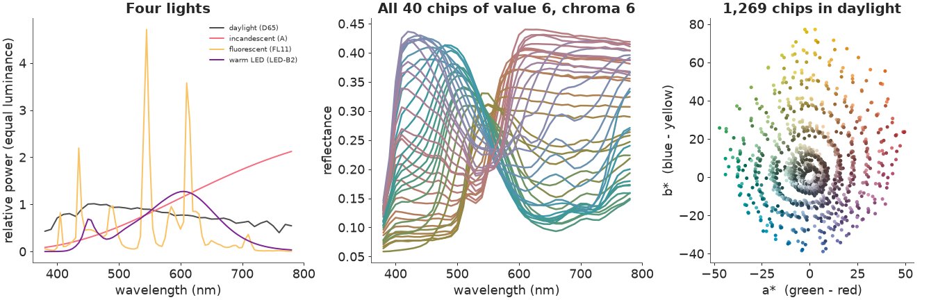
Real surface spectra are smooth, broad curves: a hue is mostly where the curve rises or peaks, chroma how much it does. Most of the chips' variety sits in a few shapes; Part C makes that precise, and it is the whole reason colour can be inverted at all. Note also that the curves keep changing above 700 nm, where the eye is almost blind: no colour measurement can say anything about that part of a spectrum.
B. What the observer cannot see
A 3 x 41 matrix and its null space
Under one light, the observer is a linear map $A$ from 41 reflectances to 3 tristimulus values, $\text{XYZ} = A R$ (CIELAB is a fixed function of XYZ). A 3 x 41 matrix has a null space of dimension 38: any spectrum $b$ with $A b = 0$ can be added to a surface without changing its colour. Wyszecki called such $b$ metameric blacks; Cohen split every spectrum into a fundamental metamer (its projection onto the three-dimensional row space of $A$, which fixes the colour) and a black (everything the observer cannot see):
$$R = \underbrace{A^\top (A A^\top)^{-1} A\, R}_{\text{fundamental}} + \underbrace{\big(I - A^\top (A A^\top)^{-1} A\big) R}_{\text{metameric black}}.$$
Swapping blacks between surfaces makes new metamers. Take one chip, keep its fundamental, and give it the black of another chip (keeping only results that stay between 0 and 1).
A_obs = W["D65"].T                                           # 3 x 41: the observer as a matrix
U, S, Vt = np.linalg.svd(A_obs)
P_FUND = A_obs.T @ np.linalg.solve(A_obs @ A_obs.T, A_obs)   # projection onto what the observer sees
print("singular values of the daylight observer:", S.round(3), f"; null space: {len(WL) - 3} dimensions")

focus = int(mun.index[mun.chip == "5GY 6/6"][0])
R0 = R_ALL[focus]
fund, black = P_FUND @ R0, R0 - P_FUND @ R0
print(f"chip {mun.chip[focus]}: size of its black relative to the spectrum {np.linalg.norm(black) / np.linalg.norm(R0):.2f}; "
      f"XYZ of the black alone: {(black @ W['D65']).round(12)}")
share = np.linalg.norm(R_ALL - R_ALL @ P_FUND.T, axis=1) / np.linalg.norm(R_ALL, axis=1)
print(f"over all chips, the black is {np.median(share):.0%} of the spectrum's size (median)")
singular values of the daylight observer: [0.382 0.298 0.113] ; null space: 38 dimensions
chip 5GY 6/6: size of its black relative to the spectrum 0.57; XYZ of the black alone: [-0.  0.  0.]
over all chips, the black is 68% of the spectrum's size (median)
More than half of this chip's spectrum (by size) is invisible to the observer, and that is typical.
How different can a metamer be? Everything with the same colour under daylight and $0 \le R \le 1$ is a polytope, so any linear function of the spectrum - for instance the redness $X - Y$ under incandescent light - is maximised and minimised at a vertex, by linear programming. Those extreme metamers are block spectra (reflectance 0 or 1 almost everywhere), the "optimal colours" of colour science: physically allowed, but nothing like real paint.
rng_b = np.random.default_rng(RANDOM_SEED + 1)
swaps = []
for j in rng_b.permutation(len(R_ALL)):
    Rm = fund + (R_ALL[j] - P_FUND @ R_ALL[j])
    if Rm.min() >= 0.01 and Rm.max() <= 0.99 and mun.hue_family[j] != mun.hue_family[focus]:
        swaps.append((mun.chip[j], Rm))
    if len(swaps) == 60:
        break


def lp_metamer(xyz_target, objective, lights=("D65",)):
    """Extreme metamer: optimise a linear objective over all 0 <= R <= 1 with the given colour(s)."""
    Aeq = np.vstack([W[k].T for k in lights])
    r = linprog(objective, A_eq=Aeq, b_eq=np.concatenate(xyz_target), bounds=[(0, 1)] * len(WL), method="highs")
    return r.x


x0 = R0 @ W["D65"]
redness_A = W["A"] @ np.array([1.0, -1.0, 0.0])              # X - Y under A: a proxy for a*
metamers = {"the chip itself": R0}
fl_shift = [de2000(lab(Rm, "FL11"), lab(R0, "FL11")) for _, Rm in swaps]
for i in np.argsort(fl_shift)[[len(swaps) // 2, -1]]:
    metamers[f"its fundamental + the black of {swaps[i][0]}"] = swaps[i][1]
metamers["linear programme: reddest under A"] = lp_metamer([x0], -redness_A)
metamers["linear programme: greenest under A"] = lp_metamer([x0], redness_A)

fig, axs = plt.subplots(len(metamers), 2, figsize=(12, 2.1 * len(metamers)),
                        gridspec_kw={"width_ratios": [1.2, 1]}, layout="none")
fig.subplots_adjust(hspace=0.55, left=0.05, right=0.99, top=0.9, bottom=0.06, wspace=0.08)
for r_, (name, Rm) in enumerate(metamers.items()):
    ax = axs[r_, 0]
    ax.fill_between(WL, 0, Rm, color=rgb(Rm))
    ax.plot(WL, R0, color="k", lw=0.9, ls="--")
    ax.set_ylim(0, 1.02)
    ax.set_xlim(380, 780)
    ax.set_title(name, fontsize=9, loc="left")
    ax.tick_params(labelsize=7)
    ax = axs[r_, 1]
    for c_, k in enumerate(LIGHTS):
        ax.add_patch(plt.Rectangle((c_, 0), 0.92, 1, color=rgb(Rm, k)))
        ax.add_patch(plt.Rectangle((c_ + 0.46, 0), 0.46, 1, color=rgb(R0, k)))
        dE = de2000(lab(Rm, k), lab(R0, k))
        ax.text(c_ + 0.46, -0.12, f"ΔE00 {dE:.1f}", ha="center", va="top", fontsize=8)
        if r_ == 0:
            ax.text(c_ + 0.46, 1.12, LIGHT_NAMES[k].replace(" (", "\n("), ha="center", fontsize=8)
    ax.set_xlim(-0.05, 4)
    ax.set_ylim(-0.45, 1.5)
    ax.axis("off")
axs[-1, 0].set_xlabel("wavelength (nm)", fontsize=9)
fig.suptitle(f"Five spectra with exactly the daylight colour of Munsell {mun.chip[focus]} (dashed: the chip).\n"
             "Split swatches: left half the spectrum, right half the chip, under each light", fontsize=10)
show_jpeg(fig)
print("largest daylight ΔE00 between any of these and the chip:",
      f"{max(de2000(lab(Rm), lab(R0)) for Rm in metamers.values()):.1e}")
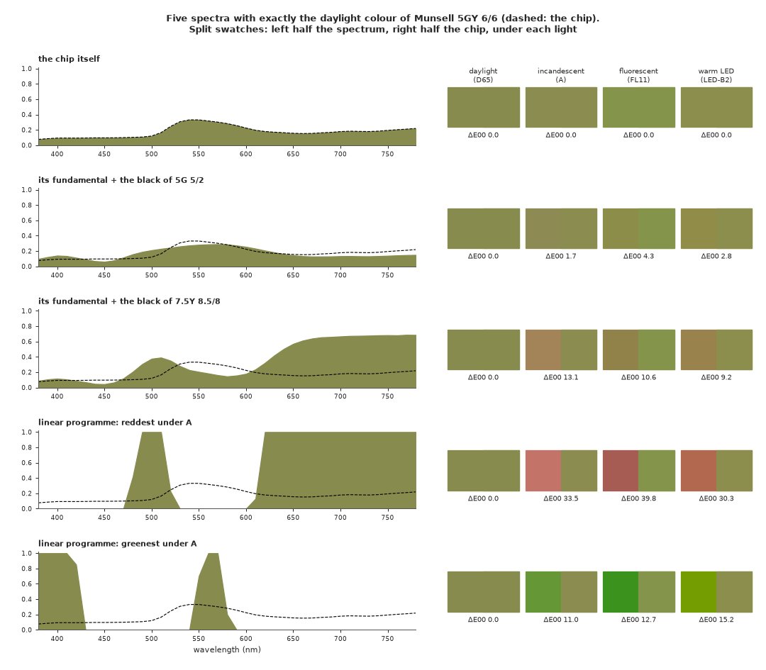
largest daylight ΔE00 between any of these and the chip: 3.9e-14
All five are the same colour in daylight: the split swatches in the first column have no visible seam, and ΔE00 is zero to rounding error. Under the other lights they come apart. The black of a greyish green chip (5G 5/2) moves the colour by 2-4 ΔE00, the black of a yellow chip (7.5Y 8.5/8) by 9-13, and the linear-programming extremes by 11 to 40, turning an olive yellow-green into brick red or grass green.
The metamer-mismatch body: every colour physics allows
Repeating the linear programme for many objectives (directions in XYZ under the second light) traces the whole convex set of colours the chip's metamers can have there, the metamer-mismatch body. It is the answer with no prior beyond $0 \le R \le 1$.
def mismatch_body(xyzs, light, lights=("D65",), n_dir=200, seed=0):
    """CIELAB under `light` of extreme metamers (0 <= R <= 1) matching the XYZ in `xyzs` under `lights`."""
    g = np.random.default_rng(seed)
    dirs = g.standard_normal((n_dir, 3))
    dirs /= np.linalg.norm(dirs, axis=1, keepdims=True)
    return xyz_to_lab(np.array([lp_metamer(xyzs, -(W[light] @ d), lights) @ W[light] for d in dirs]))


def hull_ab(lab_pts):
    h = ConvexHull(lab_pts[:, 1:])
    return lab_pts[np.r_[h.vertices, h.vertices[0]]][:, 1:]


t0 = time.time()
bodies = {k: mismatch_body([x0], k, n_dir=300) for k in ["A", "FL11", "LED_B2"]}
print(f"900 linear programmes in {time.time() - t0:.1f} s")
for k, b in bodies.items():
    print(f"{LIGHT_NAMES[k]:20s}: the most distant possible metamer is {de2000(b, lab(R0, k)).max():.0f} ΔE00 from the chip")

# real near-metamers inside the Munsell set
pairs = []
for i in range(len(R_ALL)):
    j = np.arange(i + 1, len(R_ALL))
    d = de2000(LAB["D65"][i], LAB["D65"][j])
    for jj in j[d < 1.0]:
        pairs.append((de2000(LAB["D65"][i], LAB["D65"][jj]), *[de2000(LAB[k][i], LAB[k][jj]) for k in ["A", "FL11", "LED_B2"]]))
pairs = pd.DataFrame(pairs, columns=["D65", "A", "FL11", "LED_B2"])
print(f"\n{len(pairs)} pairs of different Munsell chips are within ΔE00 < 1 of each other in daylight. Under the other lights:")
print(pairs.agg(["median", lambda x: x.quantile(0.9), "max"]).set_axis(["median", "90%", "max"]).round(2))
900 linear programmes in 0.5 s
incandescent (A)    : the most distant possible metamer is 34 ΔE00 from the chip
fluorescent (FL11)  : the most distant possible metamer is 59 ΔE00 from the chip
warm LED (LED-B2)   : the most distant possible metamer is 31 ΔE00 from the chip

64 pairs of different Munsell chips are within ΔE00 < 1 of each other in daylight. Under the other lights:
         D65     A  FL11  LED_B2
median  0.86  0.93  0.94    0.96
90%     0.97  1.16  1.37    1.21
max     1.00  2.98  3.27    2.86
Physics allows a metamer of this chip that is 59 ΔE00 away under FL11 (31-34 under the smooth lights); these bodies are the grey regions in the figures of Part D. Real surfaces do not explore that range. The Munsell set contains 64 pairs of different chips within ΔE00 1 of each other in daylight, and under the other lights they hardly drift: their median difference goes from 0.86 to 0.93-0.96, the 90th percentile to 1.2-1.4 and the largest to 3. Real metamerism is small compared with what physics permits, because real colourants have smooth, broad absorption bands. A useful prior has to know this, and that is what Part C is about.
C. Priors for spectra
Hold out a fifth of the chips (269) for validation and learn from the other 1,000. All priors live on the logit of reflectance, $\eta(\lambda) = \log\{R/(1-R)\}$, so every draw is a valid reflectance in (0, 1). Three candidates, all Gaussian on that scale:
- smooth GP - "spectra are smooth, and that's all I know": a stationary GP over wavelength (squared-exponential kernel), with its mean, amplitude and length-scale fitted to the training chips by maximum marginal likelihood (so it is not a straw man: it is the best stationary smoothness prior for these data);
- learned - the mean and full 41 x 41 covariance of the training chips' logit spectra. With 1,000 chips and 41 dimensions the parameter uncertainty is negligible (the Normal-inverse-Wishart posterior predictive is a Student-t with about 960 degrees of freedom), so we plug the estimates in;
- 3-component - the classic linear model of surface reflectance (Maloney & Wandell 1986; the principal components of Munsell spectra were first studied by Parkkinen and colleagues in 1989): the mean plus three principal components. Three unknowns for three measured numbers, so the colour determines the spectrum exactly - no metamers at all.
rng_c = np.random.default_rng(RANDOM_SEED + 2)
perm = rng_c.permutation(len(R_ALL))
test_idx, train_idx = np.sort(perm[:269]), np.sort(perm[269:])


def logit(R):
    return np.log(R / (1 - R))


Zt = logit(R_ALL[train_idx])
MU, COV = Zt.mean(0), np.cov(Zt.T)
evals, evecs = np.linalg.eigh(COV)
evals, evecs = evals[::-1], evecs[:, ::-1]
print("cumulative share of logit-spectrum variance in the first principal components:",
      (np.cumsum(evals) / evals.sum())[:6].round(3))
DIFF = WL[:, None] - WL[None]


def gp_cov(amp, ell, nug):
    return amp**2 * np.exp(-0.5 * (DIFF / ell) ** 2) + nug**2 * np.eye(len(WL))


def gauss_nll(Z, m, K):
    Lk = np.linalg.cholesky(K)
    r = np.linalg.solve(Lk, (Z - m).T)
    return 0.5 * (r**2).sum() + Z.shape[0] * (np.log(np.diag(Lk)).sum() + 0.5 * len(WL) * np.log(2 * np.pi))


res = minimize(lambda p: gauss_nll(Zt, p[0], gp_cov(*np.exp(p[1:]))), [MU.mean(), 0, np.log(50), np.log(0.05)],
               method="Nelder-Mead", options={"maxiter": 4000, "xatol": 1e-4, "fatol": 1e-3})
GP_MEAN, (GP_AMP, GP_ELL, GP_NUG) = res.x[0], np.exp(res.x[1:])
print(f"smooth GP: mean logit {GP_MEAN:.2f} (R = {1 / (1 + np.exp(-GP_MEAN)):.2f}), amplitude {GP_AMP:.2f}, "
      f"length-scale {GP_ELL:.0f} nm, nugget {GP_NUG:.3f}")

PRIORS = {
    "smooth GP": dict(mean=np.full(len(WL), GP_MEAN), chol=np.linalg.cholesky(gp_cov(GP_AMP, GP_ELL, GP_NUG))),
    "learned": dict(mean=MU, chol=np.linalg.cholesky(COV + 1e-6 * np.eye(len(WL)))),
    "3-component": dict(mean=MU, chol=evecs[:, :3] * np.sqrt(evals[:3])),
}
PRIOR_COLORS = {"smooth GP": "C0", "learned": "C1", "3-component": "k"}
Zh = logit(R_ALL[test_idx])
for name in ["smooth GP", "learned"]:
    p = PRIORS[name]
    print(f"{name:10s}: log density of the 269 held-out spectra, per chip: "
          f"{-gauss_nll(Zh, p['mean'], p['chol'] @ p['chol'].T) / len(Zh):.1f}")


def prior_draws(name, n, seed=1):
    p = PRIORS[name]
    z = np.random.default_rng(seed).standard_normal((n, p["chol"].shape[1]))
    return 1 / (1 + np.exp(-(p["mean"] + z @ p["chol"].T)))
cumulative share of logit-spectrum variance in the first principal components: [0.778 0.93 0.984 0.993 0.996 0.997]
smooth GP: mean logit -1.21 (R = 0.23), amplitude 0.83, length-scale 26 nm, nugget 0.008
smooth GP : log density of the 269 held-out spectra, per chip: 44.0
learned   : log density of the 269 held-out spectra, per chip: 89.2
Three principal components carry 98% of the (logit) variance of the training chips, six carry 99.7%: the classic finding that surface spectra are low-dimensional. The fitted smoothness GP has a length-scale of about 26 nm. On the 269 held-out spectra the learned prior is better by about 45 nats per chip, an enormous margin (the 3-component model puts no density off its three-dimensional subspace, so it cannot be scored this way).
Prior predictive check. What surfaces does each prior believe in? Draw spectra, look at their shapes and their colours, next to real chips.
fig, axs = plt.subplots(2, 4, figsize=(16, 7.5), gridspec_kw={"height_ratios": [1, 1.1]})
show = {"Munsell chips (data)": R_ALL[rng.choice(len(R_ALL), 300, replace=False)]}
show.update({f"prior: {k}": prior_draws(k, 300) for k in PRIORS})
for c_, (name, Rs) in enumerate(show.items()):
    for Rm in Rs[:25]:
        axs[0, c_].plot(WL, Rm, color=rgb(Rm), lw=1.3)
    axs[0, c_].set_ylim(0, 1)
    axs[0, c_].set_title(name)
    axs[0, c_].set_xlabel("wavelength (nm)")
    L_ = lab(Rs)
    axs[1, c_].scatter(L_[:, 1], L_[:, 2], c=lab_to_srgb(L_), s=10)
    axs[1, c_].set_xlim(-60, 80)
    axs[1, c_].set_ylim(-60, 90)
    axs[1, c_].set_xlabel("a*")
axs[0, 0].set_ylabel("reflectance")
axs[1, 0].set_ylabel("b*")
fig.suptitle("25 spectra from each prior in their daylight colours (top) and the colours of 300 (bottom)")
show_jpeg(fig)
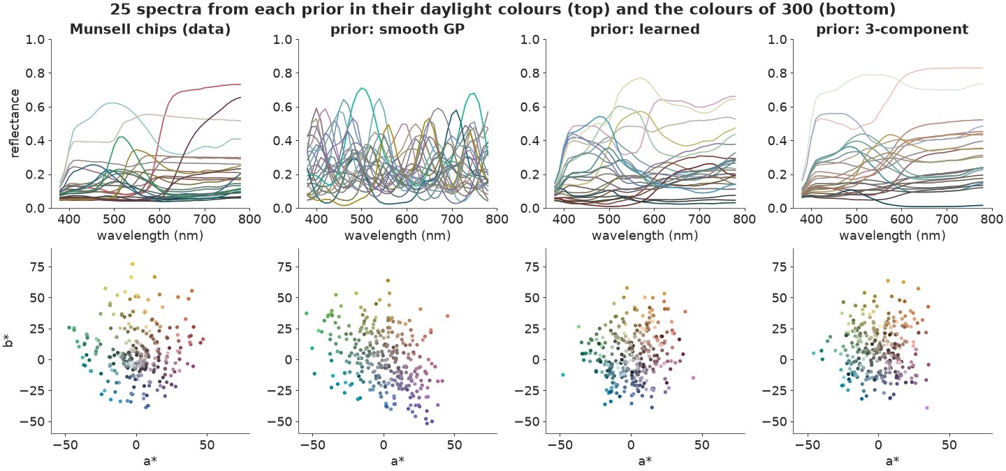
The smoothness GP produces wiggly curves with several bumps, nothing like a paint, and a colour cloud that reaches further into purples and blues than any chip. The learned prior's draws look like real chips: smooth, one or two broad features, low in the violet; their colour cloud is a little more compact than the chips' (fewer vivid yellows), since a single Gaussian cannot follow the edges of the set exactly. The 3-component draws look just as realistic - the difference will only show in the posterior.
A closed-form preview: how much can one colour tell?
Before any sampling, a linear-Gaussian calculation tells how much of a prior's uncertainty a colour measurement can remove. Approximate each prior by a Gaussian on reflectance (moments of its draws) and observe XYZ with tiny noise: the posterior covariance is the prior's minus a rank-3 update, in closed form. The share of the prior's total variance that survives is a one-number summary of "how big the metamer set is, relative to the prior".
XYZ_SD = 0.002


def variance_left(C, lights):
    G = np.vstack([W[k].T for k in lights])
    S_ = G @ C @ G.T + XYZ_SD**2 * np.eye(len(G))
    return np.trace(C - C @ G.T @ np.linalg.solve(S_, G @ C)) / np.trace(C)


prior_R_cov = {k: np.cov(prior_draws(k, 20000, seed=5).T) for k in ["smooth GP", "learned"]}
print(pd.DataFrame({k: {"daylight": variance_left(C, ["D65"]), "daylight + incandescent": variance_left(C, ["D65", "A"])}
                    for k, C in prior_R_cov.items()}).round(3).rename_axis("measured under"))
                         smooth GP  learned
measured under
daylight                     0.610    0.044
daylight + incandescent      0.457    0.029
One daylight colour removes 96% of the learned prior's variance but only 39% of the smoothness GP's: real spectra vary mostly in directions the eye can see, so the learned prior's metamer set is small. The GP spreads its variance evenly over wavelengths, in combinations the eye cannot separate. A second light helps both, but the GP stays vague. (The approximation ignores the logit and CIELAB non-linearities; PyMC does not need to.)
D. Inverting colour to spectrum in PyMC
The model for one chip, with logit-reflectance $\eta$ drawn from a prior with mean $m$ and Cholesky factor $L$:
$$z \sim \mathcal N(0, I), \qquad R = \operatorname{logit}^{-1}(m + L z), \qquad y_{\text{light}} \sim \mathcal N\big(\text{Lab}_{\text{light}}(R),\ 0.5^2 I\big).$$
The observation is a colorimeter reading: we simulate it from each held-out chip's measured
spectrum, adding noise with a standard deviation of 0.5 CIELAB units per coordinate (a typical
instrument-to-instrument agreement). Chips are independent, so 96 of the held-out chips go into
one model with a chip dimension: one compilation and one sampler run instead of 96.
SIGMA_LAB = 0.5
N_VAL = 96
rng_d = np.random.default_rng(RANDOM_SEED + 3)
val = test_idx[rng_d.choice(len(test_idx), N_VAL, replace=False)]
Y_OBS = {k: lab(R_ALL[val], k) + SIGMA_LAB * rng_d.standard_normal((N_VAL, 3)) for k in ["D65", "A"]}
coords = {"chip": mun.chip[val].to_numpy(dtype=object), "wl": WL, "lab": ["L", "a", "b"]}


def invert(prior, lights=("D65",), thin=4):
    """Posterior spectra of all validation chips given their colour under `lights`: (draw, chip, wl)."""
    p = PRIORS[prior]
    with pm.Model(coords={**coords, "k": np.arange(p["chol"].shape[1])}) as m:
        z = pm.Normal("z", 0, 1, dims=("chip", "k"))
        R = pm.Deterministic("R", pm.math.sigmoid(p["mean"] + z @ p["chol"].T), dims=("chip", "wl"))
        for k in lights:
            pm.Normal(f"y_{k}", lab_pt(R, W[k]), SIGMA_LAB, observed=Y_OBS[k], dims=("chip", "lab"))
        t0 = time.time()
        idata = pm.sample(random_seed=RANDOM_SEED, progressbar=False)
    st = idata.sample_stats
    print(f"{prior:11s} | {'+'.join(lights):6s}: {time.time() - t0:3.0f} s, divergences {int(st['diverging'].sum())}, "
          f"mean tree depth {float(st['depth'].mean()):.1f}, max r_hat(R) {float(az.rhat(idata.posterior['R']).max()):.3f}, "
          f"min bulk ESS(R) {float(az.ess(idata.posterior['R']).min()):.0f}")
    return idata.posterior["R"].isel(draw=slice(None, None, thin)).stack(s=("chain", "draw")).transpose("s", "chip", "wl").values


post = {}
for prior in PRIORS:
    post[(prior, "D65")] = invert(prior)
smooth GP | D65 : 47 s, divergences 0, mean tree depth 8.6, max r_hat(R) 1.006, min bulk ESS(R) 3163
learned | D65 : 29 s, divergences 0, mean tree depth 8.0, max r_hat(R) 1.004, min bulk ESS(R) 1684
3-component | D65 : 2 s, divergences 0, mean tree depth 4.0, max r_hat(R) 1.007, min bulk ESS(R) 3903
All three samplers are healthy: no divergences, r_hat at most 1.01, and at least about 1,700 effective draws for every one of the 96 x 41 reflectances. The tree depth of 8 (255 gradient steps per draw) for the two full priors is the geometry of the problem: in each chip 3 of 41 directions are pinned down to within the measurement noise and 38 are held only by the prior, a condition number that a diagonal mass matrix cannot remove because the pinned directions are not aligned with the coordinates. (nutpie's low-rank mass matrix did not help: in a trial on 20 chips it was 7 and 25 times slower, with hundreds of divergences for the GP prior.)
How wide is each posterior, and how close is its centre to the truth, under each light?
def spread(Rd, light):
    """Median ΔE00 between posterior draws and the posterior-median colour, per chip."""
    L_ = lab(Rd, light)
    return np.median(de2000(L_, np.median(L_, 0)), 0)


TRUE = {k: lab(R_ALL[val], k) for k in LIGHTS}
rows = []
for (prior, obs), Rd in post.items():
    for k in LIGHTS:
        rows.append((prior, LIGHT_NAMES[k], np.median(spread(Rd, k)), np.median(de2000(np.median(lab(Rd, k), 0), TRUE[k]))))
tab = pd.DataFrame(rows, columns=["prior", "light", "spread", "error"])
print("median over chips of (posterior spread | error of the posterior median), ΔE00, colour observed in daylight:")
print(tab.pivot(index="light", columns="prior").reindex([LIGHT_NAMES[k] for k in LIGHTS]).round(2))
median over chips of (posterior spread | error of the posterior median), ΔE00, colour observed in daylight:
                        spread                         error
prior              3-component learned smooth GP 3-component learned smooth GP
light
daylight (D65)            0.60    0.60      0.59        0.64    0.65      0.66
incandescent (A)          0.63    1.15      2.86        1.08    0.98      1.93
fluorescent (FL11)        0.60    1.41      5.24        1.19    1.17      1.49
warm LED (LED-B2)         0.62    1.14      3.53        1.05    1.05      1.44
In daylight, where the colour was measured, all three priors agree: spread and error about 0.6, the measurement noise. Under the other lights they part ways:
- the smooth GP is vague (a spread of 3-5 ΔE00) and its best guess is off by 1.4-1.9;
- the learned prior is sharp (spread 1.1-1.4) and its best guess is off by 1.0-1.2;
- the 3-component model is the sharpest (0.6: it believes only in the measurement noise), but its best guess is no better than the learned prior's. Its certainty is not information; Part E measures how misleading it is.
Posterior spectra, drawn in the colour they show under another light
Two held-out chips: the one where the GP and the learned prior disagree most about FL11 (a bluish grey, 10PB 6/1), and a typical colourful one (a green, 2.5G 6/8). Each thin line is one posterior spectrum, drawn in the colour it would show under the fluorescent FL11. In daylight all of them have (within the noise) the same colour; the spread of line colours is the metamer mismatch.
gp_sp, le_sp = spread(post[("smooth GP", "D65")], "FL11"), spread(post[("learned", "D65")], "FL11")
colourful = np.flatnonzero(mun.chroma.to_numpy()[val] >= 6)
SHOW = [int(np.argmax(gp_sp - le_sp)), int(colourful[np.argsort(le_sp[colourful])[len(colourful) // 2]])]
print({mun.chip[val[i]]: f"FL11 spread: GP {gp_sp[i]:.1f}, learned {le_sp[i]:.1f}" for i in SHOW})

fig, axs = plt.subplots(2, 3, figsize=(16, 8.5), sharey=True)
for r_, i in enumerate(SHOW):
    for c_, prior in enumerate(PRIORS):
        ax = axs[r_, c_]
        Rd = post[(prior, "D65")][:, i]
        for Rm, cl in zip(Rd[:80], rgb(Rd[:80], "FL11")):
            ax.plot(WL, Rm, color=cl, lw=0.9, alpha=0.85)
        lo, hi = np.quantile(Rd, [0.05, 0.95], 0)
        ax.plot(WL, lo, color="0.3", lw=0.7, ls=":")
        ax.plot(WL, hi, color="0.3", lw=0.7, ls=":")
        ax.plot(WL, R_ALL[val[i]], color="k", lw=2.2, label="measured spectrum")
        ax.set_title(f"{mun.chip[val[i]]}, prior: {prior}", fontsize=10)
        ax.set_ylim(0, 1)
    axs[r_, 0].set_ylabel("reflectance")
axs[0, 0].legend(fontsize=8)
for ax in axs[1]:
    ax.set_xlabel("wavelength (nm)")
fig.suptitle("Posterior spectra given the daylight colour only, each drawn in the colour it shows under FL11 (dotted: 90% band)")
show_jpeg(fig)
{'10PB 6/1': 'FL11 spread: GP 9.2, learned 2.3', '2.5G 6/8': 'FL11 spread: GP 4.2, learned 1.1'}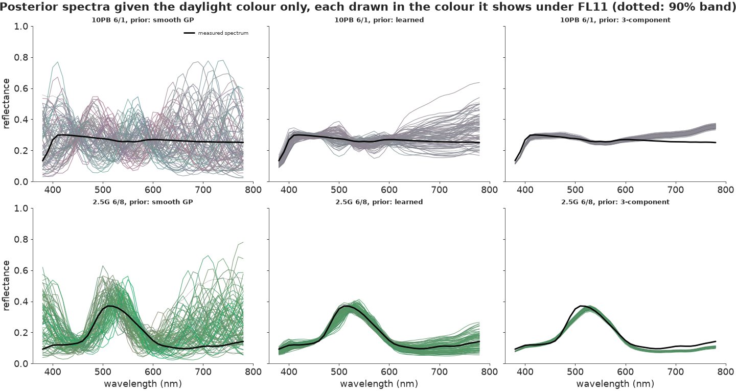
The GP's metamers are anything smooth enough with the right colour: bumpy curves that cross the true spectrum everywhere, and whose FL11 colours range from pink to teal for the grey chip. The learned prior's metamers hug the true spectrum below 600 nm and fan out mostly above 650 nm, where the eye is weakest (and where the prior, not the measurement, decides). The 3-component posterior is a thin ribbon, and it misses: above the true spectrum beyond 650 nm for the grey chip, below the green chip's peak and its long-wavelength tail. Confidently wrong.
Swatch fans: the same posterior under four lights
A spectrum is abstract; a swatch is what a client looks at. Cut each swatch into 40 vertical strips, one posterior draw each, sorted by hue, rendered under each light. A uniform swatch means a certain colour; a striped one means the metamers disagree under that light, and the stripes show how they disagree. The small inner square is the real chip.
def swatch_fan(ax, Rd, light, x0_, y0_, w=1.0, h=1.0, n=40, truth=None):
    """A swatch cut into n vertical strips, one posterior draw each, ordered by hue under the light."""
    L_ = lab(Rd[:n], light)
    cols = lab_to_srgb(L_[np.argsort(np.arctan2(L_[:, 2], L_[:, 1]))])
    for s_, c in enumerate(cols):
        ax.add_patch(plt.Rectangle((x0_ + s_ * w / n, y0_), w / n * 1.02, h, color=c, lw=0))
    if truth is not None:
        ax.add_patch(plt.Rectangle((x0_ + 0.35 * w, y0_ + 0.25 * h), 0.3 * w, 0.5 * h, facecolor=rgb(truth, light),
                                   edgecolor="white", lw=1.2))


fig, ax = plt.subplots(figsize=(12, 7))
for r_, i in enumerate(SHOW):
    for p_, prior in enumerate(PRIORS):
        y = -(r_ * 3.7 + p_ * 1.15)
        for c_, k in enumerate(LIGHTS):
            swatch_fan(ax, post[(prior, "D65")][:, i], k, c_ * 1.2, y, truth=R_ALL[val[i]])
        ax.text(-0.1, y + 0.5, f"{mun.chip[val[i]]}\nprior: {prior}", ha="right", va="center", fontsize=10)
for c_, k in enumerate(LIGHTS):
    ax.text(c_ * 1.2 + 0.5, 1.15, LIGHT_NAMES[k], ha="center", fontsize=10)
ax.set_xlim(-1.3, 4.7)
ax.set_ylim(-6.1, 1.5)
ax.axis("off")
ax.set_title("40 posterior spectra per swatch, side by side, under each light (inner square: the real chip)", fontsize=11)
show_jpeg(fig)
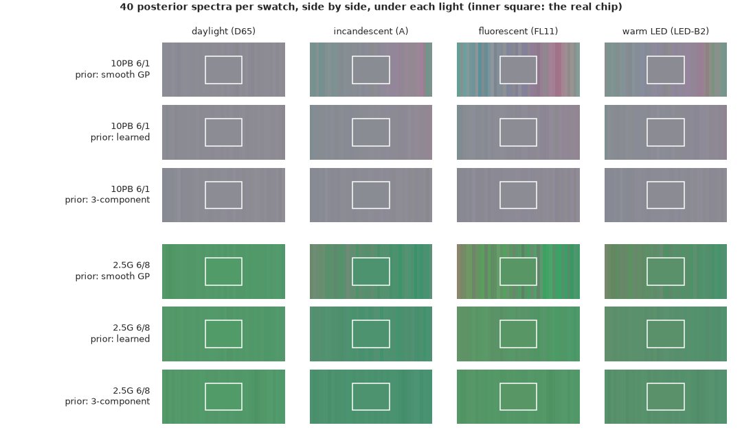
In daylight every swatch is flat: the colour was measured. Under FL11 the GP's swatches become barcodes (teal to pink for the grey chip, brown to bright green for the green one); the learned prior's show a gentle gradient that contains the real chip; the 3-component swatches stay flat under every light, which is exactly the problem.
Mismatch clouds against the physical limit
The same posteriors as points in the ab plane under each light, with 90% ellipses, inside the metamer-mismatch body (grey) - everything physics allows for a spectrum with this daylight colour. The main panels zoom on the posteriors; the insets show the whole body, with the zoomed window as a rectangle.
def ellipse(ax, pts, color, ls="-", lw=1.6, prob=0.9):
    c = np.cov(pts.T)
    vals, vecs = np.linalg.eigh(c)
    k = np.sqrt(-2 * np.log(1 - prob))
    ang = np.degrees(np.arctan2(vecs[1, 1], vecs[0, 1]))
    ax.add_patch(Ellipse(pts.mean(0), 2 * k * np.sqrt(vals[1]), 2 * k * np.sqrt(vals[0]), angle=ang,
                         fill=False, color=color, ls=ls, lw=lw))


def cloud_panel(ax, i, light, posts, body_sets, zoom_from):
    """posts: {label: (draws, colour)}; body_sets: [(xyz list, lights, fill)]."""
    t = lab(R_ALL[val[i]], light)
    ins = ax.inset_axes([0.66, 0.66, 0.33, 0.33])
    for xyzs, lights_, fc in body_sets:
        hb = hull_ab(mismatch_body(xyzs, light, lights_))
        for a_ in (ax, ins):
            a_.fill(hb[:, 0], hb[:, 1], color=fc, ec="0.45", lw=0.8, zorder=0)
    for label, (Rd, col) in posts.items():
        L_ = lab(Rd, light)[:, 1:]
        ax.scatter(L_[::3, 0], L_[::3, 1], s=5, color=col, alpha=0.25, lw=0, zorder=2)
        ellipse(ax, L_, col)
        ax.plot([], [], color=col, lw=1.6, label=label)
    ax.scatter(t[1], t[2], s=150, color=lab_to_srgb(t), edgecolor="k", lw=1.5, zorder=5)
    Z_ = lab(zoom_from, light)[:, 1:]
    lo_, hi_ = np.quantile(Z_, [0.005, 0.995], 0)
    pad = 0.15 * (hi_ - lo_).max() + 1
    ctr, half = (lo_ + hi_) / 2, (hi_ - lo_).max() / 2 + pad
    ax.set_xlim(ctr[0] - half, ctr[0] + half)
    ax.set_ylim(ctr[1] - half, ctr[1] + half)
    ins.add_patch(plt.Rectangle(ctr - half, 2 * half, 2 * half, fill=False, color="k", lw=0.8))
    ins.scatter(t[1], t[2], s=8, color="k")
    ins.set_xticks([])
    ins.set_yticks([])
    ax.set_title(f"{mun.chip[val[i]]} under {LIGHT_NAMES[light]}", fontsize=10)
    ax.set_xlabel("a*")


fig, axs = plt.subplots(2, 3, figsize=(15, 10))
for r_, i in enumerate(SHOW):
    xi = [R_ALL[val[i]] @ W["D65"]]
    for c_, k in enumerate(["A", "FL11", "LED_B2"]):
        cloud_panel(axs[r_, c_], i, k, {f"prior: {p}": (post[(p, "D65")][:, i], PRIOR_COLORS[p]) for p in PRIORS},
                    [(xi, ("D65",), "0.9")], zoom_from=post[("smooth GP", "D65")][:, i])
    axs[r_, 0].set_ylabel("b*")
h_, l_ = axs[0, 0].get_legend_handles_labels()
axs[0, 0].legend(h_ + [Patch(color="0.9", ec="0.45")], l_ + ["physically possible"], fontsize=8, loc="lower left")
fig.suptitle("Colour under another light given the daylight colour: posterior draws, 90% ellipses, physical limit (grey)");
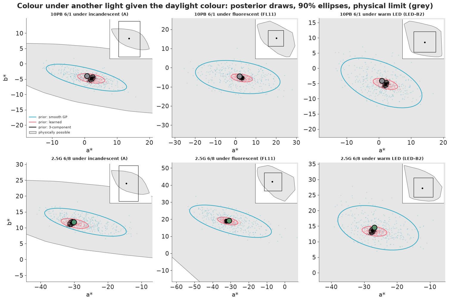
The physical bodies are enormous (the insets), and every posterior sits in a small region inside them: the prior is doing nearly all of the work. The GP's ellipses are several times the learned prior's in each direction, and the 3-component clouds are tiny. In all six panels the real colour sits inside the learned prior's 90% ellipse; it sits at the edge of, or outside, the 3-component cloud in most. All the clouds are elongated: the metamers of a chip differ mostly along one direction of the ab plane.
E. Is the posterior honest? Calibration on held-out chips
Every one of the 96 chips has a measured spectrum, so every prediction can be checked. For each chip and each coordinate (L*, a*, b*) under each light, compute the PIT, the share of posterior draws below the true value; for a calibrated posterior it is uniform, and a central interval of nominal probability $p$ contains the truth a share $p$ of the time. For the spectrum, check how often the true reflectance falls inside the 90% band, wavelength by wavelength.
LEVELS = np.array([0.5, 0.8, 0.9, 0.95])


def coverage(Rd, light):
    pit = (lab(Rd, light) < TRUE[light][None]).mean(0)                   # chip x 3
    return np.array([(np.abs(pit - 0.5) <= lv / 2).mean() for lv in LEVELS]), pit


def spectral_coverage(Rd, level=0.9):
    lo, hi = np.quantile(Rd, [(1 - level) / 2, (1 + level) / 2], 0)
    return ((R_ALL[val] >= lo) & (R_ALL[val] <= hi)).mean()


cov_rows = []
for prior in PRIORS:
    Rd = post[(prior, "D65")]
    for k in ["A", "FL11", "LED_B2"]:
        cov_rows.append((prior, f"colour under {k}", *coverage(Rd, k)[0]))
    cov_rows.append((prior, "spectrum (per wavelength)", np.nan, np.nan, spectral_coverage(Rd), np.nan))
print(f"share of truths inside central posterior intervals ({N_VAL} held-out chips, colour observed in daylight):")
print(pd.DataFrame(cov_rows, columns=["prior", "target", *[f"{int(100 * l)}%" for l in LEVELS]]).round(2).to_string(index=False))
share of truths inside central posterior intervals (96 held-out chips, colour observed in daylight):
      prior                    target  50%  80%  90%  95%
  smooth GP            colour under A 0.68 0.91 0.94 0.99
  smooth GP         colour under FL11 0.94 0.99 1.00 1.00
  smooth GP       colour under LED_B2 0.81 0.97 0.98 0.99
  smooth GP spectrum (per wavelength)  NaN  NaN 0.90  NaN
    learned            colour under A 0.56 0.84 0.93 0.97
    learned         colour under FL11 0.58 0.84 0.92 0.94
    learned       colour under LED_B2 0.55 0.84 0.93 0.97
    learned spectrum (per wavelength)  NaN  NaN 0.94  NaN
3-component            colour under A 0.37 0.62 0.74 0.80
3-component         colour under FL11 0.30 0.55 0.66 0.72
3-component       colour under LED_B2 0.36 0.62 0.71 0.77
3-component spectrum (per wavelength) NaN NaN 0.37 NaNfig, axs = plt.subplots(1, 4, figsize=(16, 4.4))
for c_, k in enumerate(["A", "FL11", "LED_B2"]):
ax = axs[c_]
for prior in PRIORS:
ax.plot(LEVELS, coverage(post[(prior, "D65")], k)[0], "o-", color=PRIOR_COLORS[prior], label=prior)
ax.plot([0.45, 1], [0.45, 1], color="0.6", ls=":")
ax.set_title(f"colour under {LIGHT_NAMES[k]}", fontsize=10)
ax.set_xlabel("nominal interval")
ax.set_ylim(0.25, 1.03)
axs[0].set_ylabel("share of true L*, a*, b* inside")
axs[0].legend(fontsize=8)
ax = axs[3]
for prior in PRIORS:
ax.hist(coverage(post[(prior, "D65")], "FL11")[1].ravel(), bins=np.linspace(0, 1, 11), histtype="step", lw=2,
color=PRIOR_COLORS[prior], density=True, label=prior)
ax.axhline(1, color="0.6", ls=":")
ax.set_xlabel("PIT of the true L*, a*, b* under FL11")
ax.set_title("PIT histogram (flat = calibrated)", fontsize=10)
fig.suptitle(f"Calibration on {N_VAL} held-out chips, colour observed in daylight only");
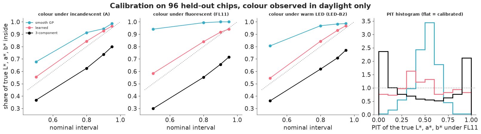
The learned prior is calibrated, if anything slightly conservative: its 50/80/90/95% intervals for the colour under each of the three other lights contain the truth 55-58%, 84%, 92-93% and 94-97% of the time, and its 90% spectral bands contain the true reflectance at 94% of wavelengths. Its PIT histogram is flat up to a mild excess in the middle (288 values: 96 chips x 3 coordinates).
The smooth GP is honest but not useful: its intervals are far too wide (the 50% intervals contain the truth 68-94% of the time, and the PIT piles up in the middle). Nothing it says is false, but "somewhere within 5 ΔE00" under FL11 is not a prediction anyone can act on.
The 3-component model is the failure of this notebook. Its nominal 90% intervals contain the truth 66-74% of the time and its 95% intervals 72-80%; its 90% spectral bands contain the true spectrum at only 37% of wavelengths; its PIT histogram is U-shaped, the signature of overconfidence. The classic linear model is not wrong about the centre (Part D: its error is close to the learned prior's), it is wrong about its uncertainty: the real chip's spectrum has components outside the three-dimensional subspace, and those are exactly the metameric blacks that make colours drift under other lights. The fix is to keep all the dimensions and let a learned prior shrink them, rather than truncate them to zero.
Where is the posterior confident, and where is it honest?
Two questions per chip. How wide is the posterior under FL11? And how surprising is the truth: a ΔE00-based PIT, the share of posterior draws closer to the posterior-median colour than the true colour is (uniform if calibrated; above 0.9 means the truth lies outside the 90% "ball").
chroma = np.hypot(TRUE["D65"][:, 1], TRUE["D65"][:, 2])
maha = np.linalg.norm(np.linalg.solve(PRIORS["learned"]["chol"], (logit(R_ALL[val]) - MU).T), axis=0)


def radial_pit(Rd, light):
    L_ = lab(Rd, light)
    med = np.median(L_, 0)
    return (de2000(L_, med) < de2000(TRUE[light], med)[None]).mean(0)


fig, axs = plt.subplots(1, 2, figsize=(14, 5))
for prior, mk in [("smooth GP", "s"), ("learned", "o")]:
    axs[0].scatter(chroma, spread(post[(prior, "D65")], "FL11"), c=rgb(R_ALL[val]), marker=mk, s=60,
                   edgecolor=PRIOR_COLORS[prior], lw=1.5, label=f"prior: {prior}")
axs[0].set_yscale("log")
axs[0].set_xlabel("chroma of the chip in daylight (C*ab)")
axs[0].set_ylabel("posterior spread under FL11 (median ΔE00)")
axs[0].legend(fontsize=8)
axs[0].set_title("Saturated colours have fewer metamers")
rp = radial_pit(post[("learned", "D65")], "FL11")
axs[1].scatter(maha, rp, c=rgb(R_ALL[val]), s=70, edgecolor="k")
axs[1].axhline(0.9, color="0.5", ls=":")
axs[1].set_xlabel("how unusual the true spectrum is (Mahalanobis distance under the learned prior)")
axs[1].set_ylabel("ΔE00-PIT of the true FL11 colour")
axs[1].set_title("... and unusual spectra surprise the learned prior")
print(f"rank correlation, spread vs chroma: GP {pd.Series(chroma).corr(pd.Series(gp_sp), method='spearman'):.2f}, "
      f"learned {pd.Series(chroma).corr(pd.Series(le_sp), method='spearman'):.2f}")
print(f"learned prior: median ΔE00-PIT {np.median(rp):.2f}; > 0.9 (truth outside the 90% ball) under FL11: {(rp > 0.9).mean():.0%} of chips; "
      f"among the quarter with the most unusual spectra {(rp[maha >= np.quantile(maha, 0.75)] > 0.9).mean():.0%}, "
      f"among the rest {(rp[maha < np.quantile(maha, 0.75)] > 0.9).mean():.0%}")
rank correlation, spread vs chroma: GP -0.76, learned -0.80
learned prior: median ΔE00-PIT 0.32; > 0.9 (truth outside the 90% ball) under FL11: 11% of chips; among the quarter with the most unusual spectra 25%, among the rest 7%
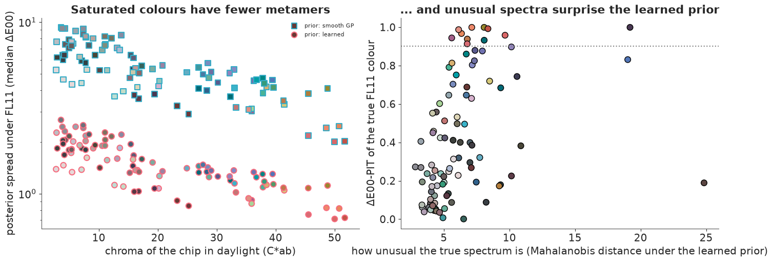
Confidence follows chroma. The more saturated the colour, the smaller the posterior, under both priors (rank correlation about -0.8): a colour near the edge of what surfaces can reach has few ways to be made, and at the very edge (the block spectra of Part B) exactly one. Greyish, low-chroma chips are the ones whose colour under another light is least predictable. This is a property of the problem, not of a prior.
Honesty follows typicality. Overall the truth falls outside the learned posterior's 90% ball for about 11% of chips, as it should. But those misses concentrate among the chips whose true spectra are most unusual for the prior (the right-hand quarter of the panel: about a quarter missed, against 7% for the rest), while for typical chips the ΔE00-PIT leans towards small values (its median over all chips is 0.32 rather than 0.5: the truth tends to be closer to the centre than the posterior expects, so for typical surfaces the learned posterior is somewhat conservative). That is the limitation of any learned prior: a surface made with a colourant the training set does not contain (a fluorescent ink, an unusual dye) will be predicted confidently and wrongly. The posterior is calibrated for surfaces like those it learned from.
F. One light or two?
A colorimeter can often measure under a second light. Measure every held-out chip under incandescent light (A) as well, 6 numbers instead of 3, and predict the colour under FL11 and the LED.
post[("learned", "D65+A")] = invert("learned", ("D65", "A"))
rows = []
for obs in ["D65", "D65+A"]:
    Rd = post[("learned", obs)]
    for k in ["FL11", "LED_B2"]:
        rows.append((obs, f"colour under {k}", np.median(spread(Rd, k)), coverage(Rd, k)[0][2]))
    rows.append((obs, "spectrum", np.median(np.diff(np.quantile(Rd, [0.05, 0.95], 0), axis=0)), spectral_coverage(Rd)))
print(pd.DataFrame(rows, columns=["observed under", "predicted", "median spread (ΔE00) or 90% band width", "90% coverage"])
      .round(3).to_string(index=False))
learned | D65+A : 64 s, divergences 0, mean tree depth 9.0, max r_hat(R) 1.005, min bulk ESS(R) 3522
observed under           predicted  median spread (ΔE00) or 90% band width  90% coverage
           D65   colour under FL11                                   1.410         0.917
           D65 colour under LED_B2                                   1.139         0.931
           D65            spectrum                                   0.076         0.936
         D65+A   colour under FL11                                   0.970         0.913
         D65+A colour under LED_B2                                   0.607         0.931
         D65+A            spectrum                                   0.055         0.925
i = SHOW[0]
xi, xa = R_ALL[val[i]] @ W["D65"], R_ALL[val[i]] @ W["A"]
fig, axs = plt.subplots(1, 3, figsize=(16, 5.2))
for ax, k in zip(axs[:2], ["FL11", "LED_B2"]):
cloud_panel(ax, i, k, {"posterior, daylight only": (post[("learned", "D65")][:, i], "C1"),
"posterior, daylight + A": (post[("learned", "D65+A")][:, i], "C4")},
[([xi], ("D65",), "0.93"), ([xi, xa], ("D65", "A"), "0.8")],
zoom_from=post[("learned", "D65")][:, i])
axs[0].set_ylabel("b*")
h_, l_ = axs[0].get_legend_handles_labels()
axs[0].legend(h_ + [Patch(color="0.93", ec="0.45"), Patch(color="0.8", ec="0.45")],
l_ + ["possible given daylight", "possible given daylight + A"], fontsize=8, loc="lower left")
ax = axs[2]
sp1, sp2 = spread(post[("learned", "D65")], "FL11"), spread(post[("learned", "D65+A")], "FL11")
ax.scatter(sp1, sp2, c=rgb(R_ALL[val]), s=60, edgecolor="k")
lim = max(sp1.max(), sp2.max()) * 1.05
ax.plot([0, lim], [0, lim], color="0.6", ls=":")
ax.set_xlabel("spread under FL11, daylight only (ΔE00)")
ax.set_ylabel("... daylight + incandescent")
ax.set_title("A second light, chip by chip", fontsize=10)
print(f"ratio of spreads under FL11 (two lights / one): median {np.median(sp2 / sp1):.2f}")
ratio of spreads under FL11 (two lights / one): median 0.67
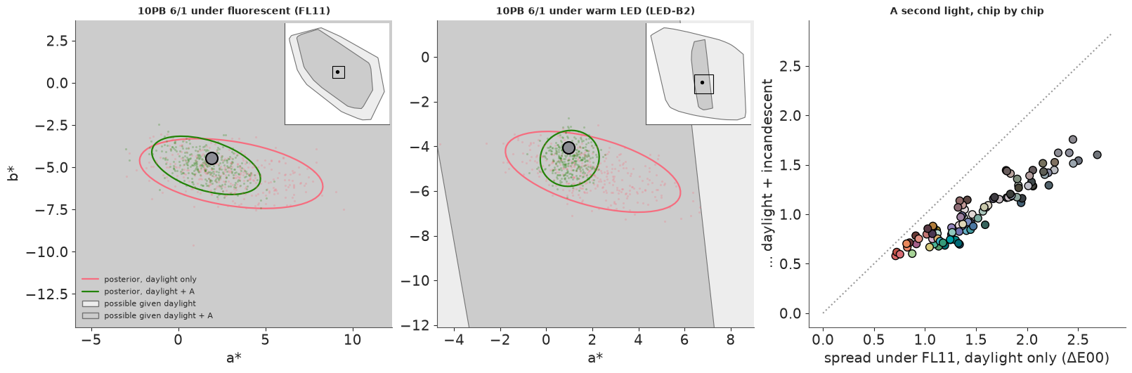
The second measurement shrinks the predicted FL11 spread by about a third (1.4 to 1.0 ΔE00, median) and the LED spread by about half (1.1 to 0.6), while the coverage of the 90% intervals stays at 91-93%: the posterior gets sharper without getting overconfident. The LED gains most because the warm LED and incandescent light have similar, smooth red-heavy spectra: measuring under one nearly fixes the colour under the other. The physical bodies say the same thing (the darker grey region in the inset of the LED panel is a thin sliver). FL11's spiky spectrum probes combinations of wavelengths neither smooth light does, so some uncertainty remains. A second light works on every chip (right panel: all points below the diagonal), most for the grey, uncertain ones.
G. A decision: matching a sample for a gallery
A gallery wants a wall to match a client's sample. The sample was measured with a colorimeter in daylight (and, in a second version, under incandescent light too). The gallery is lit by a mix of daylight and warm LEDs whose balance changes through the day: a share $w$ of daylight, with $w \sim \text{Beta}(2, 2)$. The loss is the ΔE00 between wall and sample under the gallery light, averaged over $w$. Two versions of the choice:
- Pick a chip. Choose one of the 1,000 training chips (a "fan deck") for the wall. The naive rule takes the chip closest to the sample's daylight reading.
- Pick a recipe. A supplier mixes a white base with three of eleven tints. Many recipes match the sample in daylight - metamers again, now among the candidates - and the naive rule takes the one with the least pigment (the cheapest). As a stand-in for a paint-formulation system: the tints are the most saturated training chip of each hue family plus a near-black, the base the lightest near-neutral chip, and mixtures follow single-constant Kubelka-Munk (as in E74, K/S is additive: $K/S_\text{mix} = \sum_j c_j\, K/S_j$ with fractions $c_j \ge 0$ summing to one). For each sample every one of the 165 three-tint recipes is fitted to the daylight reading (Levenberg-Marquardt on the fractions, all recipes at once), and those within ΔE00 0.5 are the candidates.
The Bayes rule picks the candidate with the smallest loss averaged over $w$ and over the posterior spectra of the sample. The oracle knows the sample's true spectrum: the best anyone could do. Every held-out chip plays the sample once, so every rule is scored on the truth.
def ks(R):
    return (1 - R) ** 2 / (2 * R)


def km(K):
    return 1 + K - np.sqrt(K**2 + 2 * K)


tr = mun.loc[train_idx]
TINTS = [int(tr[tr.hue_family == f].chroma.idxmax()) for f in ["R", "YR", "Y", "GY", "G", "BG", "B", "PB", "P", "RP"]]
TINTS.append(int(tr[tr.value == tr.value.min()].chroma.idxmin()))
WHITE = int(tr[tr.value == tr.value.max()].chroma.idxmin())
KW, KT = ks(R_ALL[WHITE]), ks(R_ALL[TINTS])
RECIPES = np.array(list(combinations(range(len(TINTS)), 3)))
print(f"white base {mun.chip[WHITE]}; tints {', '.join(mun.chip[TINTS])}; {len(RECIPES)} recipes")


def mix(u):
    """Recipes' reflectance from logits u (recipe x 3) of the three tints against the white base."""
    e = np.exp(np.concatenate([np.zeros((len(u), 1)), u], 1))
    c = e / e.sum(1, keepdims=True)
    return km(c[:, :1] * KW + np.einsum("rj,rjw->rw", c[:, 1:], KT[RECIPES])), c


def fit_recipes(y, iters=40):
    """Levenberg-Marquardt for all recipes at once: fractions whose daylight colour matches y."""
    u, lam = np.full((len(RECIPES), 3), -1.0), np.full(len(RECIPES), 1e-2)

    def resid(u_):
        return lab(mix(u_)[0]) - y
    r = resid(u)
    for _ in range(iters):
        J = np.stack([(resid(u + 1e-5 * np.eye(3)[k]) - r) / 1e-5 for k in range(3)], -1)
        step = np.linalg.solve(np.einsum("nij,nik->njk", J, J) + lam[:, None, None] * np.eye(3),
                               -np.einsum("nij,ni->nj", J, r)[..., None])[..., 0]
        un = np.clip(u + step, -12, 12)
        rn = resid(un)
        better = (rn**2).sum(1) < (r**2).sum(1)
        u, r = np.where(better[:, None], un, u), np.where(better[:, None], rn, r)
        lam = np.where(better, lam / 3, lam * 4)
    R, c = mix(u)
    return R, c, de2000(lab(R), y)


LED, D65s = light_spd("LED_B2"), light_spd("D65")
W_GRID = np.linspace(0, 1, 11)
W_PROB = beta_dist(2, 2).pdf(W_GRID)
W_PROB /= W_PROB.sum()
W_MIX = [observer(w * D65s / (D65s * CMF[:, 1]).sum() + (1 - w) * LED / (LED * CMF[:, 1]).sum()) for w in W_GRID]


def gallery_lab(R):
    return np.stack([lab(R, Wm) for Wm in W_MIX])              # w x ... x 3


def gallery_loss(lab_a, lab_b):
    """ΔE00 averaged over the daylight share w (axis 0)."""
    return np.tensordot(W_PROB, de2000(lab_a, lab_b), axes=(0, 0))


BAYES = {"Bayes, smooth GP": ("smooth GP", "D65"), "Bayes, learned": ("learned", "D65"),
         "Bayes, learned, daylight + A": ("learned", "D65+A")}


def decide(lab_cand, true_loss, ci):
    """True loss of the Bayes pick for each posterior; lab_cand is w x candidate x 3."""
    out = {}
    for label, key in BAYES.items():
        lab_post = gallery_lab(post[key][::4, ci])                  # w x draw x 3
        exp_loss = np.array([gallery_loss(lab_cand[:, r][:, None], lab_post).mean() for r in range(lab_cand.shape[1])])
        out[label] = true_loss[np.argmin(exp_loss)]
    return out


t0 = time.time()
train_gal = gallery_lab(R_ALL[train_idx])
chips_dec, recipe_dec = [], []
for ci in range(N_VAL):
    truth_gal = gallery_lab(R_ALL[val[ci]])[:, None]
    # 1. a chip from the fan deck: candidates are the 40 closest in daylight
    cand = np.argsort(de2000(LAB["D65"][train_idx], Y_OBS["D65"][ci]))[:40]
    tl = gallery_loss(train_gal[:, cand], truth_gal)
    chips_dec.append({"naive": tl[0], **decide(train_gal[:, cand], tl, ci), "oracle": tl.min()})
    # 2. a recipe
    Rrec, c, dE = fit_recipes(Y_OBS["D65"][ci])
    ok = np.flatnonzero(dE < 0.5)
    if len(ok) >= 2:
        lab_rec = gallery_lab(Rrec[ok])
        tl = gallery_loss(lab_rec, truth_gal)
        recipe_dec.append({"target": ci, "random daylight match": tl.mean(), "naive": tl[np.argmin(c[ok, 1:].sum(1))],
                           **decide(lab_rec, tl, ci), "oracle": tl.min()})
chips_dec, recipe_dec = pd.DataFrame(chips_dec), pd.DataFrame(recipe_dec)
print(f"{time.time() - t0:.0f} s; {len(recipe_dec)} of {N_VAL} samples can be matched by at least two recipes")
RULES = ["naive", *BAYES, "oracle"]
rows = {}
for name, d in [("pick a chip", chips_dec), ("pick a recipe", recipe_dec)]:
    diff = d[RULES].sub(d["naive"], axis=0)
    rows[(name, "mean ΔE00")] = d[RULES].mean()
    rows[(name, "vs naive")] = diff.mean()
    rows[(name, "± s.e.")] = diff.std() / np.sqrt(len(d))
    rows[(name, "share > 1")] = (d[RULES] > 1).mean()
dec_table = pd.DataFrame(rows).rename(index={"naive": "naive (nearest in daylight / least pigment)"})
print(dec_table.round(3))
print(f"recipes, a random daylight match: {recipe_dec['random daylight match'].mean():.2f}")
white base 5R 9/1; tints 5R 6/14, 2.5YR 6/14, 2.5Y 8/12, 2.5GY 8.5/10, 2.5G 6/12, 2.5BG 6/10, 10B 6/10, 5PB 4/12, 10P 5/12, 2.5RP 6/12, 5R 2.5/1; 165 recipes
7 s; 55 of 96 samples can be matched by at least two recipes
                                            pick a chip                           pick a recipe
                                              mean ΔE00 vs naive ± s.e. share > 1     mean ΔE00 vs naive ± s.e. share > 1
naive (nearest in daylight / least pigment)       2.233    0.000  0.000     0.927         0.801    0.000  0.000     0.255
Bayes, smooth GP                                  2.347    0.114  0.048     0.938         0.799   -0.002  0.030     0.236
Bayes, learned                                    2.299    0.066  0.034     0.938         0.787   -0.014  0.025     0.236
Bayes, learned, daylight + A                      2.166   -0.067  0.024     0.917         0.659   -0.142  0.028     0.109
oracle                                            2.142   -0.091  0.024     0.917         0.616   -0.185  0.029     0.091
recipes, a random daylight match: 0.89fig, axs = plt.subplots(1, 3, figsize=(16, 4.8), gridspec_kw={"width_ratios": [1.2, 1.2, 1]})
for ax, (name, d) in zip(axs[:2], [("pick a chip (1,000 candidates)", chips_dec), ("pick a recipe (daylight matches)", recipe_dec)]):
diff = d[RULES].sub(d["naive"], axis=0)
m, se = diff.mean(), diff.std() / np.sqrt(len(d))
cols = ["0.5", "C0", "C1", "C4", "k"]
ax.barh(range(len(RULES)), m.values, xerr=1.96 * se.values, color=cols, height=0.6)
ax.set_yticks(range(len(RULES)))
ax.set_yticklabels(["naive", *BAYES, "oracle"] if ax is axs[0] else [""] * len(RULES))
ax.axvline(0, color="k", lw=0.8)
ax.invert_yaxis()
ax.set_xlabel("gallery ΔE00 minus naive (mean, 95% CI)")
ax.set_title(f"{name}: naive = {d['naive'].mean():.2f} ΔE00", fontsize=10)
ax = axs[2]
tg = recipe_dec.target.to_numpy()
ax.scatter(recipe_dec["naive"], recipe_dec["Bayes, learned, daylight + A"], c=rgb(R_ALL[val[tg]]), s=60, edgecolor="k")
lim = recipe_dec[["naive", "Bayes, learned, daylight + A"]].to_numpy().max() * 1.05
ax.plot([0, lim], [0, lim], color="0.6", ls=":")
ax.axhline(1, color="0.8", lw=0.8)
ax.axvline(1, color="0.8", lw=0.8)
ax.set_xlabel("least-pigment recipe: gallery ΔE00")
ax.set_ylabel("Bayes, daylight + A: gallery ΔE00")
ax.set_title("Recipes, sample by sample", fontsize=10);
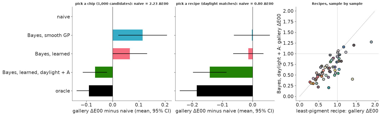
Reading the table and the figure:
- Picking a recipe. A random daylight match leaves the wall 0.89 ΔE00 from the sample in the gallery, the least-pigment rule 0.80, and the oracle 0.62. With one daylight reading the Bayes rule is no better than least pigment (the difference, -0.01 ± 0.03, is noise), whichever prior it uses. With a second reading under incandescent light it closes about three-quarters of the gap to the oracle (0.66 ΔE00) and cuts the share of walls with a visible mismatch (> 1 ΔE00) from about a quarter to 11%, close to the oracle's 9%.
- Picking a chip. The fan deck is coarse (even the oracle's pick is 2.1 ΔE00 from the sample on average), so nearly every pick is visibly off whatever the rule, and the oracle beats the naive rule by only 0.09 ΔE00. Here the one-light Bayes rules are worse than naive, by 0.07 ± 0.03 (learned) and 0.11 ± 0.05 (GP). Two lights again beat the naive rule, by 0.07, most of what the oracle gains.
So a calibrated posterior did not, by itself, make a better decision than a simple rule. Why did the naive chip rule win? Taking the chip nearest in daylight quietly uses a second prior: the target's neighbours in the Munsell set, whose spectra (similar pigments, similar colour) shift with the light much as the target's does. The learned prior is one Gaussian for the whole set and knows nothing local. A direct check: predict each sample's colour under the other lights as its daylight reading plus the colour shift of its nearest training chip, and compare with the posterior median.
nb_rows = []
for k in ["A", "FL11", "LED_B2"]:
    e_nb, e_post = [], []
    for ci in range(N_VAL):
        nn = train_idx[np.argmin(de2000(LAB["D65"][train_idx], Y_OBS["D65"][ci]))]
        e_nb.append(de2000(Y_OBS["D65"][ci] + LAB[k][nn] - LAB["D65"][nn], TRUE[k][ci]))
        e_post.append(de2000(np.median(lab(post[("learned", "D65")][:, ci], k), 0), TRUE[k][ci]))
    nb_rows.append((LIGHT_NAMES[k], np.median(e_nb), np.median(e_post)))
print(pd.DataFrame(nb_rows, columns=["light", "nearest chip's shift", "posterior median (learned)"])
      .set_index("light").round(2).rename_axis("median ΔE00 error of the predicted colour"))
                                           nearest chip's shift  posterior median (learned)
median ΔE00 error of the predicted colour
incandescent (A)                                           0.91                        0.98
fluorescent (FL11)                                         0.89                        1.17
warm LED (LED-B2)                                          0.93                        1.05
The nearest chip's colour shift predicts the colour under the other lights better than the learned posterior does, most clearly under FL11. The learned prior is calibrated but not the sharpest prior these data support: the Munsell spectra lie on a curved, lumpy set (a hue circle at every lightness), and a single Gaussian fills in the gaps between the lumps. That is the next model to build (see "Try it yourself"). Calibration is necessary for good decisions, not sufficient; and here the most valuable thing the posterior did was tell us that a second measurement was worth taking.
H. Walking through the metamers
An animation for the bluish grey chip of Part D. The top row walks through physically possible metamers (points halfway between the chip and linear-programming extremes, which are exact metamers too, since the colour is linear in the spectrum); the bottom row through plausible ones, posterior draws under the learned prior. Left: the spectrum (drawn in its daylight colour) against the chip's own (dashed). Right: a swatch under daylight and under FL11, with the real chip as the inner rectangle of each half.
i = SHOW[0]
Rt = R_ALL[val[i]]
xt = Rt @ W["D65"]
FLW = W["FL11"]
ext = [lp_metamer([xt], -(FLW @ np.array([np.cos(a), np.sin(a), -0.5 * (np.cos(a) + np.sin(a))])))
       for a in np.linspace(0, 2 * np.pi, 7)[:-1]]
Rd = post[("learned", "D65")][:, i]
LA = lab(Rd, "FL11")
hue = np.arctan2(LA[:, 2] - LA[:, 2].mean(), LA[:, 1] - LA[:, 1].mean())
plaus = [Rd[np.argmin(np.abs(hue - h))] for h in np.linspace(-np.pi, np.pi, 7)[:-1]]


def walk(keys, steps=7):
    keys = keys + keys[:1]
    return np.concatenate([np.linspace(0, 1, steps, endpoint=False)[:, None] * (b - a)[None] + a[None]
                           for a, b in zip(keys[:-1], keys[1:])])


paths = [walk([0.5 * e + 0.5 * Rt for e in ext]), walk(plaus)]
print(f"{len(paths[0])} frames; largest daylight ΔE00 from the chip along each path: "
      f"{[round(float(de2000(lab(p), lab(Rt)).max()), 2) for p in paths]}")

fig, axs = plt.subplots(2, 2, figsize=(8.4, 5.4), dpi=72, gridspec_kw={"width_ratios": [1.7, 1]}, layout="none")
fig.subplots_adjust(left=0.07, right=0.98, bottom=0.1, top=0.9, wspace=0.12, hspace=0.45)
arts = []
for r_, (p, name) in enumerate(zip(paths, ["physically possible metamers", "plausible metamers (learned prior)"])):
    ax = axs[r_, 0]
    ax.plot(WL, Rt, color="k", lw=1, ls="--")
    line, = ax.plot(WL, p[0], lw=2.5, color=rgb(p[0]))
    ax.set_ylim(0, 1)
    ax.set_title(name, fontsize=9)
    ax.tick_params(labelsize=7)
    ax = axs[r_, 1]
    ax.axis("off")
    im = ax.imshow(np.zeros((10, 20, 3)))
    ax.text(5, -1.2, "daylight", ha="center", fontsize=8)
    ax.text(15, -1.2, "FL11", ha="center", fontsize=8)
    txt = ax.text(10, 11.8, "", ha="center", fontsize=8)
    arts.append((line, im, txt))
axs[1, 0].set_xlabel("wavelength (nm)", fontsize=8)


def swatch_img(Rm):
    img = np.zeros((10, 20, 3))
    for c_, k in enumerate(["D65", "FL11"]):
        img[:, 10 * c_:10 * c_ + 10] = rgb(Rm, k)
        img[2:8, 10 * c_ + 5:10 * c_ + 9] = rgb(Rt, k)
    return img


def update(f):
    out = []
    for (line, im, txt), p in zip(arts, paths):
        line.set_ydata(p[f])
        line.set_color(rgb(p[f]))
        im.set_data(swatch_img(p[f]))
        txt.set_text(f"FL11: ΔE00 {de2000(lab(p[f], 'FL11'), lab(Rt, 'FL11')):.1f} from the chip")
        out += [line, im, txt]
    return out


anim = animation.FuncAnimation(fig, update, frames=len(paths[0]), interval=180)
plt.close(fig)
plt.rcParams["animation.frame_format"] = "jpeg"          # swatches: JPEG frames are far smaller
display(HTML(anim.to_jshtml(default_mode="loop")))
plt.rcParams["animation.frame_format"] = "png"
42 frames; largest daylight ΔE00 from the chip along each path: [0.0, 1.5]
Along the top path the spectrum jumps between blocks and the daylight half of the swatch never changes, while the FL11 half swings through strongly coloured yellow-greens, greens and purples, 20-28 ΔE00 from the chip. Along the bottom path the spectrum barely moves below 650 nm, and the FL11 half shifts by 1.5-4 ΔE00 around the chip. Both rows are "the same colour"; only one of them is what real surfaces do. (The plausible path is built from posterior draws, which match the noisy reading, so its daylight colour wanders by up to 1.5 ΔE00; the physical path is exact.)
Summary
- A colour is a projection. Under one light the observer is a 3 x 41 matrix; the 38 directions it cannot see (metameric blacks) can be added to any surface without changing its colour. Linear programming gives the exact set of colours those metamers can have under another light: tens of ΔE00 wide. Real surfaces use a tiny part of it: near-metameric Munsell pairs stay within 1-3.
- The prior does the work. A smoothness-only GP leaves a vague metamer set (3-5 ΔE00 under the other lights); with a covariance learned from 1,000 measured surfaces, one daylight colour removes 96% of the prior variance, the colour under incandescent, fluorescent and LED light is predicted to about 1 ΔE00, and the predictions are calibrated on held-out chips. The textbook 3-component linear model gives about the same best guess but claims about half the spread it should (its 90% intervals cover 66-74%).
- Batch small independent inversions into one model (a
chipdimension): one compilation, one sampler run, 96 posteriors. Expect deep trees: 3 of 41 directions are pinned by data. - Validate predictions, not parameters: coverage of spectral bands, and above all the PIT and interval coverage of the colour under lights that were not measured. Confidence follows chroma (saturated colours have few metamers); honesty follows typicality (unusual spectra are the misses).
- Information beats cleverness. One more reading under a second light shrinks the predicted spread by a third to a half and makes the Bayes decision clearly better than simple rules; with one reading, a naive nearest-chip rule did as well or better, because it silently used a local prior the global Gaussian lacks.
- When colour is the uncertainty, show colour: spaghetti of spectra drawn in their rendered colours, swatch fans, split swatches and the animation make metamer mismatch visible directly; ab clouds against the physical body and calibration plots make it quantitative.
Try it yourself
- A local prior. Replace the single Gaussian by a mixture: k-means (or the hue families) on the
training logit-spectra, one mean and covariance per cluster, and the cluster summed out inside the
model with
pt.logsumexp(or a kernel prior centred on every training spectrum). Does the posterior get sharper under FL11 while the 90% coverage stays near 90%? Does the one-light Bayes rule now beat the nearest-chip rule of Part G? - Which second light? Repeat Part F with the second reading under FL11 or LED-B2 instead of A
(and try FL2 and LED-B4 from
cie_illuminants_e76). Which single extra light best predicts the others? Before measuring anything, the closed-form linear-Gaussian calculation of Part C ranks the candidates: does its ranking agree with the full posterior? - A camera as the observer. Replace the second light by a second observer: a camera's three spectral sensitivities (published measurements exist for dozens of camera models) under daylight. How much does one photograph shrink the metamer set compared with a colorimeter under a second light, and where in the spectrum does the camera see what the eye does not?