The setting
Many measurements live on a circle. A wind blows from a direction between 0 and 360 degrees, and 359 degrees is next to 1 degree. An animal walks past a camera at a time of day, and 23:59 is next to 00:01. A disease peaks in a season, and December is next to January. The usual toolbox quietly assumes a line: an average, a normal likelihood, a regression slope, a histogram with two ends. On a circle each of these can give a confident, wrong answer.
We work with three real datasets, each making a different point:
- Wind at Santa Barbara. The airport sits on a coastal plain between the Pacific and the Santa Ynez mountains. On a typical day, cool air drains down from the mountains towards the sea at night and the sea breeze blows inland in the afternoon. The direction therefore swings through half the compass every day, and the swing changes with the season. How does the wind direction depend on wind speed, hour and season, and how sure are we?
- Camera traps in a tropical forest. Ocelots hunt at night. Do their hours overlap with those of the agouti (active by day), the paca and the spiny rat (active by night)? The standard answer in ecology is an overlap coefficient between two activity curves on the 24-hour circle. How big is it and how uncertain?
- Earthquakes as a control. Magnitude 3+ earthquakes in Oklahoma should not care what time it is. What does "no daily pattern" look like, and how does a Bayesian model say so?
| part | question | tool |
|---|---|---|
| A | Why are angles different? | mean resultant vector, four circular distributions, a null dataset |
| B | What does the Santa Barbara wind do? | calms, rounding, local solar time, rose diagrams by hour |
| C | Does the direction depend on wind speed? | tan-half link, a wrapped prior, a second mode, the canonical link |
| D | How does it depend on hour and season? | von Mises and projected-normal regression, a mixture of regimes, circular PPCs, LOO, a held-out year |
| E | When is an ocelot about, and when are its prey? | von Mises mixtures and label switching, a log-Fourier density, overlap and activity level |
Everything is written with NumPy, SciPy and PyMC; there is no circular-statistics package.
import logging
import time
import warnings

import arviz as az
import matplotlib.pyplot as plt
import numpy as np
import pandas as pd
import pymc as pm
import pytensor.tensor as pt
import xarray as xr
from matplotlib.patches import FancyArrowPatch
from scipy import special
from scipy.optimize import brentq

from pymc_challenges import data

RANDOM_SEED = 81
rng = np.random.default_rng(RANDOM_SEED)
az.style.use("arviz-variat")
logging.getLogger("pymc").setLevel(logging.WARNING)
warnings.filterwarnings("ignore", category=RuntimeWarning, module="arviz")
warnings.filterwarnings("ignore", message=".*sample_stats.*")
pd.set_option("display.width", 170)
pd.set_option("display.max_columns", 20)
T_START = time.time()

BLUE, ORANGE, AQUA = "#2a78d6", "#eb6834", "#1baf7a"   # categorical slots 1-3, fixed order
INK, MUTED, LIGHT = "#0b0b0b", "#8a8984", "#d9d8d3"
TWO_PI = 2 * np.pi


def wrap(a):
    """Angle(s) to (-pi, pi]."""
    return np.angle(np.exp(1j * np.asarray(a)))


def mean_resultant(th, axis=None):
    """Mean direction and mean resultant length of angles in radians."""
    z = np.exp(1j * np.asarray(th)).mean(axis=axis)
    return np.angle(z), np.abs(z)


def A1(k):
    """Mean resultant length of a von Mises with concentration k: I1(k) / I0(k)."""
    return special.i1e(k) / special.i0e(k)


def A1inv(R):
    return brentq(lambda k: A1(k) - R, 1e-9, 1e4) if R > 1e-9 else 0.0


def vm_logpdf(th, e1, e2):
    """von Mises log density in NATURAL parameters: exp(e1 cos th + e2 sin th) / (2 pi I0(|e|))."""
    k = np.hypot(e1, e2)
    return e1 * np.cos(th) + e2 * np.sin(th) - np.log(TWO_PI) - (np.log(special.i0e(k)) + k)


def pn_logpdf(th, m1, m2):
    """Projected normal (identity covariance) log density of the angle of z ~ N((m1, m2), I)."""
    u = m1 * np.cos(th) + m2 * np.sin(th)
    return -np.log(TWO_PI) - 0.5 * (m1 ** 2 + m2 ** 2) + np.log1p(u * np.sqrt(np.pi / 2) * special.erfcx(-u / np.sqrt(2)))


def vm_lp(th, e1, e2):
    """The same von Mises log density as a PyTensor expression."""
    k = pt.sqrt(e1 ** 2 + e2 ** 2)
    return e1 * np.cos(th) + e2 * np.sin(th) - np.log(TWO_PI) - pt.log(pt.i0(k))


def loo_from_ll(ll):
    """PSIS-LOO from a (draws, observations) log-likelihood matrix computed in NumPy."""
    tree = xr.DataTree.from_dict({
        "posterior": xr.Dataset({"d": (("chain", "draw"), np.zeros((1, ll.shape[0])))}),
        "log_likelihood": xr.Dataset({"y": (("chain", "draw", "obs"), ll[None])}),
    })
    res = az.loo(tree, pointwise=True)
    res.log_weights = None
    return res


def circ_hdi(draws, prob=0.94):
    """Shortest arc containing `prob` of the draws (valid when they cover less than a half circle)."""
    c, _ = mean_resultant(draws)
    d = np.sort(wrap(draws - c))
    m = int(np.ceil(prob * len(d)))
    widths = d[m - 1:] - d[:len(d) - m + 1]
    i = np.argmin(widths)
    return c + d[i], c + d[i + m - 1], c


def compass(ax, labels=True):
    """Polar axes as a compass: north up, clockwise, degrees FROM which the wind blows."""
    ax.set_theta_zero_location("N")
    ax.set_theta_direction(-1)
    ax.set_xticks(np.deg2rad([0, 45, 90, 135, 180, 225, 270, 315]))
    ax.set_xticklabels(["N", "NE", "E", "SE", "S", "SW", "W", "NW"] if labels else [])
    ax.grid(alpha=0.4)


def clockface(ax):
    """Polar axes as a 24-hour clock: midnight up, clockwise."""
    ax.set_theta_zero_location("N")
    ax.set_theta_direction(-1)
    ax.set_xticks(np.deg2rad(np.arange(0, 360, 45)))
    ax.set_xticklabels([f"{h:02d}:00" for h in range(0, 24, 3)], fontsize=8)
    ax.grid(alpha=0.4)
A. Angles are not numbers on a line
The arithmetic mean of angles
Two winds, one from 350 degrees (just west of north) and one from 10 degrees (just east of north), average to 180 degrees - due south - if you add the numbers and divide by two. The fix is to average the unit vectors $(\cos\theta_i, \sin\theta_i)$ instead:
$$\bar C = \frac1n \sum_i \cos\theta_i,\qquad \bar S = \frac1n \sum_i \sin\theta_i,\qquad \bar\theta = \operatorname{atan2}(\bar S, \bar C),\qquad \bar R = \sqrt{\bar C^2 + \bar S^2}.$$
$\bar\theta$ is the mean direction and $\bar R \in [0, 1]$ the mean resultant length: 1 if all angles agree, near 0 if they point every which way or if they cluster in two opposite directions. $\bar R$ plays the role of a (reverse) standard deviation; $1 - \bar R$ is the circular variance.
The Santa Barbara wind reports show how badly the arithmetic mean can go wrong on real data.
data.describe("ksba_wind")
raw = data.load("ksba_wind")
raw["utc"] = pd.to_datetime(raw.valid)
raw["lst"] = raw.utc - pd.Timedelta(hours=8)          # Pacific STANDARD time all year: see Part B
print(f"{len(raw):,} hourly reports; calm (speed 0): {np.mean(raw.sknt == 0):.1%}; "
      f"direction missing: {raw.drct.isna().mean():.1%}")

toy = np.deg2rad([350.0, 10.0])
print(f"350 and 10 degrees: arithmetic mean {np.rad2deg(toy).mean():.0f}, "
      f"circular mean {round(np.rad2deg(mean_resultant(toy)[0])) % 360:.0f}")

wind = raw[(raw.sknt > 0) & raw.drct.notna()].copy()
wind["theta"] = wrap(np.deg2rad(wind.drct))
by_month = wind.groupby(wind.lst.dt.month).agg(
    arithmetic_mean=("drct", "mean"),
    circular_mean=("theta", lambda t: np.rad2deg(mean_resultant(t)[0]) % 360),
    R=("theta", lambda t: mean_resultant(t)[1]))
print(by_month.round(2).T.to_string())
ksba_wind: Routine hourly METAR reports, 2021-01-01 to 2023-12-31 (26,101 rows, at minute 53 of each hour): valid (UTC timestamp), drct (direction the wind blows FROM, degrees clockwise from true north, reported in steps of 10; 0 together with sknt = 0 means calm), sknt (speed, knots), tmpf and dwpf (air and dew-point temperature, Fahrenheit). Empty = missing (e.g. variable direction).
  source: Iowa Environmental Mesonet (IEM, Iowa State University) ASOS/METAR archive, station SBA (Santa Barbara Municipal Airport, California; an FAA/NWS Automated Surface Observing System). Public US government observations redistributed by IEM, which asks to be acknowledged. BUILT by tools/build_e81_circular.py (the URL returns an uncompressed CSV) - keep the cached file.
  url:    https://mesonet.agron.iastate.edu/cgi-bin/request/asos.py?station=SBA&data=drct&data=sknt&data=tmpf&data=dwpf&year1=2021&month1=1&day1=1&year2=2024&month2=1&day2=1&tz=Etc/UTC&format=onlycomma&latlon=no&missing=empty&trace=empty&direct=no&report_type=3
26,101 hourly reports; calm (speed 0): 27.5%; direction missing: 3.4%
350 and 10 degrees: arithmetic mean 180, circular mean 0
lst                  1       2       3       4       5       6       7       8       9       10      11      12
arithmetic_mean  181.83  208.51  197.95  183.72  181.27  173.42  169.22  171.48  170.67  181.23  171.84  172.40
circular_mean    217.16  274.82  247.40  183.87  184.51  173.57  169.65  172.57  175.67  199.01  179.18  109.69
R                  0.04    0.30    0.17    0.22    0.30    0.34    0.43    0.38    0.28    0.23    0.08    0.02
In every month the arithmetic mean lands between 169 and 209 degrees, largely because the numbers run from 10 to 360 and average out near the middle. The circular mean moves much more (from 110 degrees in December to 275 in February) - but in December and January $\bar R$ is only 0.02-0.04: the winds of those months come from all round the compass, largely from two nearly opposite directions (Part B), so any single mean direction describes almost nothing. On a circle, a mean direction should always be reported with $\bar R$.
Four distributions on the circle
The circular analogue of the normal distribution is not unique. Four are in common use, each built a different way:
- von Mises $\text{VM}(\mu, \kappa)$: density $\propto \exp\{\kappa\cos(\theta - \mu)\}$, normalised by $2\pi I_0(\kappa)$ (a Bessel function). The maximum-entropy distribution for a given mean resultant vector, and an exponential family: $\kappa\cos(\theta-\mu) = \eta_1\cos\theta + \eta_2\sin\theta$ with natural parameters $\eta = \kappa(\cos\mu, \sin\mu)$. This fact does a lot of work in Part C.
- wrapped normal: take $x \sim N(\mu, \sigma^2)$ on the line and wind it round the circle, $\theta = x \bmod 2\pi$; the density is an infinite sum over windings.
- wrapped Cauchy: the same with a Cauchy; closed form $\frac{1-\rho^2}{2\pi(1 + \rho^2 - 2\rho\cos(\theta-\mu))}$, and heavy tails.
- projected normal: take a 2-D vector $z \sim N(m, I)$ and keep only its angle, $\theta = \operatorname{atan2}(z_2, z_1)$. The length $|z|$ is thrown away. With a general covariance it can be skewed or bimodal; with the identity it is symmetric about $\operatorname{atan2}(m_2, m_1)$.
Here they are with the same mean direction and the same mean resultant length, $\bar R = 0.6$.
R_target = 0.6
grid = np.linspace(-np.pi, np.pi, 721)
k_vm = A1inv(R_target)
sig_wn = np.sqrt(-2 * np.log(R_target))                     # wrapped normal: R = exp(-sigma^2 / 2)
dens = {
    f"von Mises (kappa = {k_vm:.2f})": np.exp(vm_logpdf(grid, k_vm, 0.0)),
    f"wrapped normal (sigma = {sig_wn:.2f})": sum(np.exp(-(grid + TWO_PI * j) ** 2 / (2 * sig_wn ** 2))
                                                 for j in range(-4, 5)) / np.sqrt(TWO_PI * sig_wn ** 2),
    "wrapped Cauchy (rho = 0.60)": (1 - R_target ** 2) / (TWO_PI * (1 + R_target ** 2 - 2 * R_target * np.cos(grid))),
}
# projected normal: find |m| giving R = 0.6 (R = E cos(theta) under the density)
dth = grid[1] - grid[0]
pn_R = lambda m: np.sum(np.cos(grid[:-1]) * np.exp(pn_logpdf(grid[:-1], m, 0.0))) * dth
m_pn = brentq(lambda m: pn_R(m) - R_target, 0.01, 10)
dens[f"projected normal (|m| = {m_pn:.2f})"] = np.exp(pn_logpdf(grid, m_pn, 0.0))

fig = plt.figure(figsize=(11, 4.2))
ax = fig.add_subplot(1, 2, 1)
axp = fig.add_subplot(1, 2, 2, projection="polar")
cols = [BLUE, ORANGE, AQUA, INK]
for (lab, d), c in zip(dens.items(), cols):
    print(f"{lab:36s} integrates to {np.sum(d[:-1]) * dth:.4f}; peak {d.max():.3f}; "
          f"density opposite the mean {d[0]:.3f}")
    ax.plot(np.rad2deg(grid), d, color=c, lw=2, label=lab)
    axp.plot(grid, d, color=c, lw=2)
ax.set(xlabel="angle from the mean direction (degrees)", ylabel="density (per radian)",
       xticks=[-180, -90, 0, 90, 180], title="Same mean direction, same mean resultant length 0.6")
ax.legend(fontsize=8)
axp.set_theta_zero_location("N")
axp.set_theta_direction(-1)
axp.set_title("The same densities on the circle", fontsize=10);
von Mises (kappa = 1.52)             integrates to 1.0000; peak 0.436; density opposite the mean 0.021
wrapped normal (sigma = 1.01)        integrates to 1.0000; peak 0.395; density opposite the mean 0.006
wrapped Cauchy (rho = 0.60)          integrates to 1.0000; peak 0.637; density opposite the mean 0.040
projected normal (|m| = 1.10)        integrates to 1.0000; peak 0.467; density opposite the mean 0.027
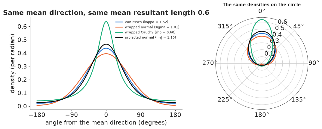
At equal $\bar R$ the von Mises and the wrapped normal are almost indistinguishable (at larger $\kappa$ they converge; in practice the von Mises is used because its density has a closed form). The wrapped Cauchy has a sharper peak and more mass far from the mean: it is the heavy-tailed option. The projected normal is flatter at the top. Which shape suits a dataset is an empirical question that LOO can answer - we will do that for the wind in Part D.
What does nothing look like?
Before looking for patterns, a control. Oklahoma's magnitude 3+ earthquakes (2005-2019) were mostly induced by wastewater injection, which runs day and night. Their times of day, in local time:
quakes = data.load("oklahoma_quakes")
t_local = pd.to_datetime(quakes.time, utc=True).dt.tz_convert("America/Chicago")
q_hour = (t_local.dt.hour + t_local.dt.minute / 60).to_numpy()
q_th = TWO_PI * q_hour / 24
n_q = len(q_th)
q_mean, q_R = mean_resultant(q_th)
Z = n_q * q_R ** 2
print(f"n = {n_q}; mean resultant length R = {q_R:.4f}; mean hour {np.rad2deg(q_mean) % 360 / 15:.1f}")
print(f"expected R under uniformity, sqrt(pi / 4n) = {np.sqrt(np.pi / (4 * n_q)):.4f}; "
      f"Rayleigh statistic nR^2 = {Z:.2f}, p ~ exp(-nR^2) = {np.exp(-Z):.2f}")

with pm.Model() as m_quake:
    eta = pm.Normal("eta", 0, 1, shape=2)                  # natural parameters of a von Mises
    kappa = pm.Deterministic("kappa", pt.sqrt(pt.sum(eta ** 2)))
    pm.Potential("ll", pt.sum(vm_lp(q_th, eta[0], eta[1])))
    idata_q = pm.sample(random_seed=RANDOM_SEED, progressbar=False)
kq = idata_q.posterior["kappa"].values.ravel()
eq = az.extract(idata_q, var_names=["eta"]).values.T
ll_q = vm_logpdf(q_th[None, :], eq[::4, 0:1], eq[::4, 1:2])
loo_q = loo_from_ll(ll_q)
print(f"posterior kappa: median {np.median(kq):.3f}, 94% upper bound {np.quantile(kq, 0.94):.3f}; "
      f"implied R at the upper bound {A1(np.quantile(kq, 0.94)):.3f}")
print(f"elpd: uniform {-n_q * np.log(TWO_PI):.1f}, von Mises {loo_q.elpd:.1f} +- {loo_q.se:.1f} "
      f"(difference {loo_q.elpd + n_q * np.log(TWO_PI):.1f})")

fig = plt.figure(figsize=(10, 4))
ax = fig.add_subplot(1, 2, 1, projection="polar")
clockface(ax)
cnt, edges = np.histogram(q_th, bins=24, range=(0, TWO_PI))
ax.bar(edges[:-1] + np.pi / 24, cnt / n_q, width=TWO_PI / 24 * 0.9, color=BLUE, alpha=0.8)
ax.plot(np.linspace(0, TWO_PI, 200), np.full(200, 1 / 24), color=INK, lw=1, ls="--")
ax.set_yticklabels([])
ax.set_title("Oklahoma M3+ earthquakes by hour\n(dashed: uniform, 1/24)", fontsize=10)
ax = fig.add_subplot(1, 2, 2)
ax.hist(kq, bins=60, color=BLUE, alpha=0.8)
ax.set(xlabel="von Mises concentration kappa", ylabel="posterior draws",
       title="Posterior of the concentration kappa");
n = 2917; mean resultant length R = 0.0215; mean hour 13.8
expected R under uniformity, sqrt(pi / 4n) = 0.0164; Rayleigh statistic nR^2 = 1.35, p ~ exp(-nR^2) = 0.26
posterior kappa: median 0.051, 94% upper bound 0.089; implied R at the upper bound 0.044
elpd: uniform -5361.1, von Mises -5361.7 +- 1.7 (difference -0.6)
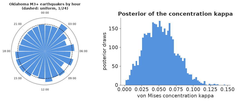
The histogram by hour looks bumpy, but each bar holds only about 120 quakes, so bumps of ±10% are noise. The mean resultant length of 0.02 is close to what 2,917 uniformly scattered times give on average (0.016): $\bar R$ is biased upwards and never exactly 0 in a finite sample, so it cannot be read on its own. The Rayleigh test does not reject uniformity.
The Bayesian version fits a von Mises and asks how concentrated it is. The posterior of $\kappa$ sits close to 0 (median 0.05; $\kappa$ is the length of a 2-D vector here, so like any length its posterior thins out towards exactly 0). Even its 94% upper bound, 0.09, implies a mean resultant length of about 0.04 - a daily cycle too weak to matter. LOO says the same in its own currency: the extra flexibility buys nothing (the uniform is 0.6 nats better, with a standard error of 1.7). Note the parameterisation: we sampled the natural parameters $\eta = \kappa(\cos\mu, \sin\mu)$, not $(\mu, \kappa)$. When $\kappa \approx 0$ the mean direction $\mu$ is meaningless and would wander over the whole circle; in $\eta$ the posterior is a harmless blob around the origin. That idea returns throughout.
B. The wind at Santa Barbara
Three details of the data matter before any model:
- Calms. When the wind speed is 0 the direction is undefined, and the report says 0 degrees. Treating 27% of the hours as north winds would invent a strong northerly mode. There are also no speeds of 1 or 2 knots in the file: the lightest winds are reported as calm. We drop calms and model the direction given a wind of at least 3 knots.
- Rounding. ASOS reports the direction in steps of 10 degrees. With the concentrations we will see ($\kappa \le 5$, an angular spread of 25 degrees or more) a 10-degree bin barely matters for the likelihood, but it matters for residual checks, where we will jitter within the bin.
- Which clock? The sea breeze follows the sun, not the clock. Daylight-saving time shifts the clock by an hour for eight months of the year, which would smear every hour-of-day effect. We use Pacific standard time (UTC - 8) all year. At Santa Barbara solar noon is then close to 12:00 (within about 20 minutes over the year).
We fit on 2021-2022 and keep 2023 aside to check predictions on data the models never saw.
wind["hour"] = wind.lst.dt.hour + wind.lst.dt.minute / 60
wind["doy"] = (wind.lst.dt.dayofyear - 1 + wind.hour / 24) / 365.25        # fraction of the year
wind["year"] = wind.lst.dt.year
train = wind[wind.year < 2023].reset_index(drop=True)
test = wind[wind.year == 2023].reset_index(drop=True)
th = train.theta.to_numpy()
n_tr = len(th)
print(f"training reports (2021-2022, not calm): {n_tr:,}; held-out 2023: {len(test):,}")
print("directions are multiples of 10 degrees:", bool(np.all(train.drct % 10 == 0)))

blocks = [(h, h + 3) for h in range(0, 24, 3)]
fig, axes = plt.subplots(2, 4, figsize=(12, 6.4), subplot_kw={"projection": "polar"})
for ax, (h0, h1) in zip(axes.ravel(), blocks):
    sel = (train.hour >= h0) & (train.hour < h1)
    t = np.deg2rad(train.drct[sel])
    cnt, edges = np.histogram(np.mod(t, TWO_PI), bins=36, range=(-np.pi / 36, TWO_PI - np.pi / 36))
    ax.bar(edges[:-1] + np.pi / 36, cnt / sel.sum(), width=TWO_PI / 36 * 0.9, color=BLUE)
    mu_b, R_b = mean_resultant(t)
    compass(ax, labels=True)
    rmax = ax.get_ylim()[1]
    ax.annotate("", xy=(mu_b, R_b * rmax), xytext=(0, 0), zorder=5,
                arrowprops=dict(arrowstyle="-|>", color=ORANGE, lw=2.5))
    ax.set_yticklabels([])
    ax.set_title(f"{h0:02d}:00-{h1:02d}:00  (R = {R_b:.2f})", fontsize=10)
fig.suptitle("Where the wind blows FROM at Santa Barbara, 2021-2022, by time of day (bars: share of reports in "
             "10-degree bins; arrow: mean resultant vector,\nfull radius = length 1)", fontsize=10);
training reports (2021-2022, not calm): 12,023; held-out 2023: 6,026
directions are multiples of 10 degrees: True
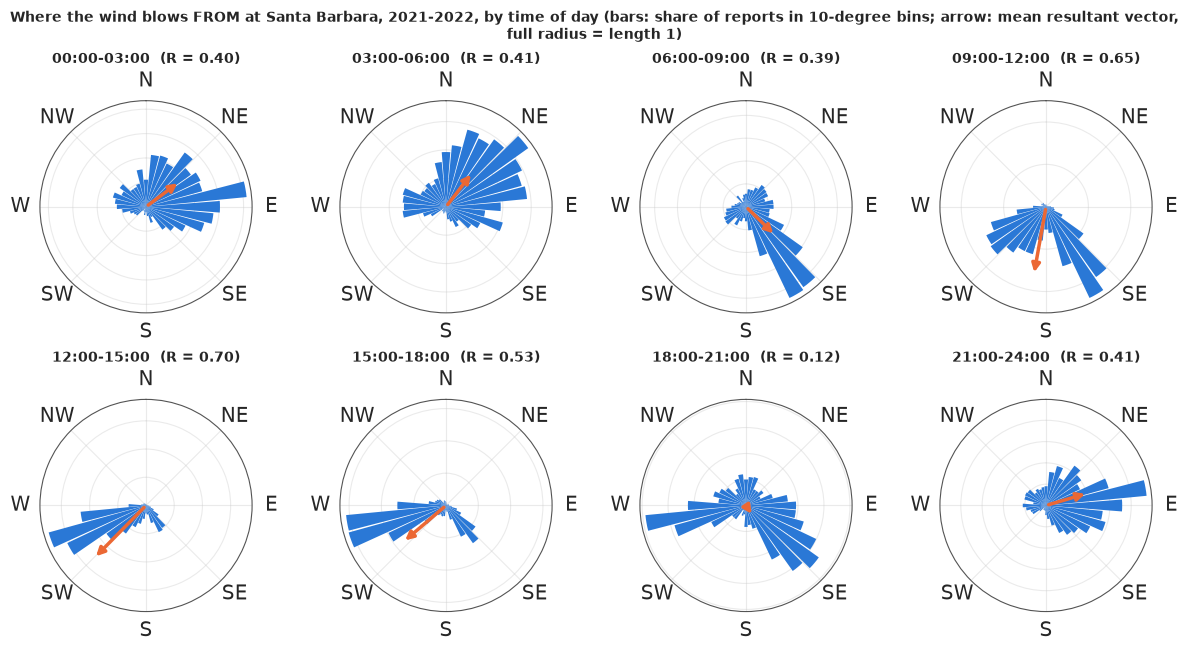
A rose diagram is a histogram wrapped round a compass. Read the eight clocks in order:
- night (21:00-06:00): a broad spread of winds from the east and northeast - air draining off the mountains and along the coast - with a small group from the west;
- morning (06:00-12:00): first the south-southeast, then two groups at once, south-southeast and west-southwest, as the sea breeze sets in;
- afternoon (12:00-18:00): the sea breeze from the west-southwest (240-270 degrees), by far the most concentrated wind of the day ($\bar R$ = 0.70);
- evening (18:00-21:00): again two groups, the dying sea breeze from the west and a group from the southeast. The mean resultant vector points between them and is short ($\bar R$ = 0.12): in this block it describes neither.
A model with one mean direction per hour can follow the daily swing; the evening block already suggests it will need more than one direction at a time.
C. Does the direction depend on wind speed? Link functions on the circle
Strong winds here are westerlies; the lightest winds come from the northeast. Regressing a circular response on a linear covariate $x$ (here the standardised log wind speed) needs a link function that maps the real line into angles. The classic choice (Fisher & Lee 1992) is the tan-half link
$$\mu(x) = \mu_0 + 2\arctan(\beta x),$$
which moves the mean direction smoothly from $\mu_0 - \pi$ to $\mu_0 + \pi$ as $x$ runs over the line, with $\theta \sim \text{VM}(\mu(x), \kappa)$. It has two traps, and it is worth seeing both before the fix.
Trap 1: the likelihood has a second mode where the link becomes a step
For fixed $\beta$ the best $\mu_0$ and $\kappa$ have closed forms (the mean direction and the inverted $A_1(\kappa) = \bar R$ of the angles $\theta_i - 2\arctan(\beta x_i)$), so the profile log-likelihood of $\beta$ costs nothing to compute.
x_sp = np.log(train.sknt.to_numpy())
X_MEAN, X_SD = x_sp.mean(), x_sp.std()
x_sp = (x_sp - X_MEAN) / X_SD


def tanhalf_profile(beta, th=th, x=x_sp):
    mu0, R = mean_resultant(th - 2 * np.arctan(beta * x))
    k = A1inv(R)
    return len(th) * (k * R - np.log(TWO_PI) - np.log(special.i0e(k)) - k), mu0, k


betas = np.r_[-np.logspace(2, -2, 90), 0.0, np.logspace(-2, 2, 90)]
prof = np.array([tanhalf_profile(b) for b in betas])
i_best = np.argmax(prof[:, 0])
neg = betas < -0.2
i_step = np.flatnonzero(neg)[np.argmax(prof[neg, 0])]
print(f"best: beta = {betas[i_best]:.2f}, mu0 = {np.rad2deg(prof[i_best, 1]) % 360:.0f} deg, "
      f"kappa = {prof[i_best, 2]:.2f}, log-lik {prof[i_best, 0]:.0f}")
print(f"second mode: beta = {betas[i_step]:.0f}, mu0 = {np.rad2deg(prof[i_step, 1]) % 360:.0f} deg, "
      f"kappa = {prof[i_step, 2]:.2f}, log-lik {prof[i_step, 0]:.0f}")
i_valley = np.flatnonzero((betas < 0) & (betas > betas[i_step]))[np.argmin(prof[(betas < 0) & (betas > betas[i_step]), 0])]
print(f"the valley between them: beta = {betas[i_valley]:.2f}, log-lik {prof[i_valley, 0]:.0f}")

fig, axes = plt.subplots(1, 2, figsize=(12, 4))
axes[0].plot(betas, prof[:, 0] - prof[i_best, 0], color=BLUE, lw=2)
axes[0].set_xscale("symlog", linthresh=0.05)
axes[0].set_xticks([-100, -10, -1, -0.1, 0, 0.1, 1, 10, 100])
axes[0].set_xticklabels(["-100", "-10", "-1", "-0.1", "0", "0.1", "1", "10", "100"])
axes[0].set(xlabel="beta (symmetric log scale)", ylabel="profile log-likelihood (relative to the best)",
            title="Profile likelihood of the tan-half slope", ylim=(-2000, 150))
axes[0].annotate("main mode", (betas[i_best], 0), xytext=(2, -600), arrowprops=dict(arrowstyle="->"))
axes[0].annotate("step-function mode", (betas[i_step], prof[i_step, 0] - prof[i_best, 0]),
                 xytext=(-60, -300), arrowprops=dict(arrowstyle="->"))
xs = np.linspace(-2.5, 2.5, 200)
sub = rng.choice(n_tr, 3000, replace=False)
axes[1].scatter(x_sp[sub] + rng.uniform(-0.05, 0.05, 3000), np.mod(train.drct.to_numpy()[sub] + rng.uniform(-5, 5, 3000), 360),
                s=2, color=MUTED, alpha=0.4)
for i, c, lab in ((i_best, BLUE, "main mode"), (i_step, ORANGE, "step-function mode")):
    mu = np.rad2deg(prof[i, 1] + 2 * np.arctan(betas[i] * xs)) % 360
    mu[np.abs(np.diff(mu, append=mu[-1])) > 180] = np.nan
    axes[1].plot(xs, mu, color=c, lw=2.5, label=f"{lab}: beta = {betas[i]:.2g}")
axes[1].set(xlabel="standardised log wind speed", ylabel="direction FROM (degrees)", yticks=range(0, 361, 90),
            title="The two modes (grey: 3,000 reports, jittered)")
axes[1].legend(fontsize=8, loc="lower right");
best: beta = 0.63, mu0 = 165 deg, kappa = 0.76, log-lik -20523
second mode: beta = -48, mu0 = 4 deg, kappa = 0.46, log-lik -21493
the valley between them: beta = -0.95, log-lik -22083
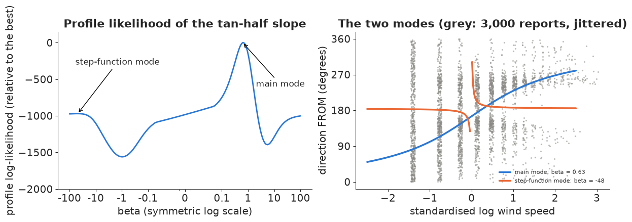
The main mode ($\beta \approx 0.6$) turns the mean direction from the northeast for light winds through the south to the west for strong winds. But the profile does not fall away as $|\beta|$ grows: for large negative $\beta$ it climbs again to a plateau (and, less high, for large positive $\beta$). There $2\arctan(\beta x)$ is a step of $\pm\pi$ at $x = 0$: the model says "light winds come from one direction and strong winds from exactly the opposite one", which is a crude but not absurd description of these data. It is about 970 log-likelihood units worse than the main mode, and separated from it by a valley 1,560 units below the main mode. (Speeds are whole knots, so the log speeds form the vertical stripes in the right panel.) A sampler that starts on the wrong side of the valley will stay there.
Trap 2: a wrapped prior on the intercept
The obvious prior for an angle is $\mu_0 \sim \text{Uniform}(-\pi, \pi)$. PyMC maps an interval to the real line with a logit transform, so $-\pi$ and $\pi$ become $-\infty$ and $+\infty$: two points that are the same direction are infinitely far apart for the sampler. Here the best $\mu_0$ is about 165 degrees (2.9 radians), close to that seam. We fit this "obvious" model with nutpie's default settings.
with pm.Model() as m_tanhalf_uniform:
    mu0 = pm.Uniform("mu0", -np.pi, np.pi)
    beta = pm.Normal("beta", 0, 2)
    kappa = pm.Gamma("kappa", 2.0, 1.0)
    pm.VonMises("y", mu=mu0 + 2 * pt.arctan(beta * x_sp), kappa=kappa, observed=th)
    idata_th_u = pm.sample(random_seed=RANDOM_SEED, progressbar=False)


def per_chain(idata, names, deg=()):
    out = {}
    for v in names:
        a = idata.posterior[v].values
        out[v] = (np.rad2deg(mean_resultant(a, axis=1)[0]) % 360) if v in deg else a.mean(1)
    out["mean logp"] = idata.sample_stats["logp"].values.mean(1)
    out["divergences"] = idata.sample_stats["diverging"].values.sum(1)
    return pd.DataFrame(out, index=[f"chain {c}" for c in range(len(out["mean logp"]))])


print(az.summary(idata_th_u, var_names=["mu0", "beta", "kappa"], round_to=3).to_string())
print(per_chain(idata_th_u, ["mu0", "beta", "kappa"], deg=("mu0",)).round(2).to_string())
        mean     sd  eti89_lb  eti89_ub  ess_bulk  ess_tail  r_hat  mcse_mean  mcse_sd
mu0   -0.076  2.126    -3.141     2.884     4.900    10.978  2.411      1.059    0.530
beta  -9.185  9.825   -20.224     0.668     5.250    10.815  2.099      4.882    0.011
kappa  0.597  0.152     0.429     0.774     5.444    11.623  1.983      0.076    0.005
            mu0   beta  kappa  mean logp  divergences
chain 0  359.07 -18.96   0.45  -21574.92            0
chain 1  180.08   0.57   0.73  -20638.85            0
chain 2  164.41   0.66   0.76  -20529.04            0
chain 3  359.09 -19.01   0.45  -21574.83            0
Everything a careless check looks at is fine: zero divergences, no warnings about step size. But $\hat R$ is about 2, and the per-chain means show why - the four chains found three different answers:
- two chains sit at a very large negative $\beta$: the step-function mode of trap 1;
- one chain found the main mode ($\beta \approx 0.6$, $\mu_0 \approx 165$ degrees);
- one chain has $\mu_0$ pressed against $-\pi$: it wants to reach 165 degrees by going the short way round through 180, and the wall of the uniform prior does not let it. Its $\beta$ matches the main mode; its mean log density is lower than that chain's.
Only the per-chain view (and $\hat R$) reveals this; divergences never will. The wall is the known cure's target: sample the direction as a point in the plane and take its angle. We give the intercept its natural parameters $\eta_0 = \kappa(\cos\mu_0, \sin\mu_0)$ with a normal prior, so $\kappa = |\eta_0|$ and $\mu_0 = \operatorname{atan2}(\eta_{0,2}, \eta_{0,1})$ - an unconstrained plane with no seam. (Sampling a free point $(c, s)$ and using only its angle also works, but its length is then set only by the prior, and the sampler funnels near the origin; tying the length to $\kappa$ lets the data identify it.)
with pm.Model() as m_tanhalf_plane:
    eta0 = pm.Normal("eta0", 0, 2, shape=2)
    mu0 = pm.Deterministic("mu0", pt.arctan2(eta0[1], eta0[0]))
    kappa = pm.Deterministic("kappa", pt.sqrt(pt.sum(eta0 ** 2)))
    beta = pm.Normal("beta", 0, 2)
    pm.VonMises("y", mu=mu0 + 2 * pt.arctan(beta * x_sp), kappa=kappa, observed=th)
    idata_th_p = pm.sample(random_seed=RANDOM_SEED, progressbar=False)
print(per_chain(idata_th_p, ["mu0", "beta", "kappa"], deg=("mu0",)).round(2).to_string())
            mu0   beta  kappa  mean logp  divergences
chain 0  164.40   0.66   0.76  -20527.95            0
chain 1  358.99 -19.00   0.44  -21574.72            0
chain 2  164.47   0.66   0.76  -20527.88            0
chain 3  164.41   0.65   0.76  -20527.73            0
No chain is stuck at a wall any more - but the step-function mode is still there, because it is a property of the likelihood, not of the parameterisation of $\mu_0$. With this seed, chains land in it again. One could start every chain in the main mode (and we do below, to compare), but that hides the problem rather than removing it.
The fix: the canonical link
Section A noted that the von Mises is an exponential family in $\eta = \kappa(\cos\mu, \sin\mu)$:
$$\log p(\theta \mid \eta) = \eta_1\cos\theta + \eta_2\sin\theta - \log\{2\pi I_0(|\eta|)\}.$$
The log normaliser is convex in $\eta$, so the log-likelihood is concave in $\eta$. If $\eta$ is a linear function of the coefficients - $\eta(x) = a + b\,x + c\,x^2$ with vectors $a, b, c \in \mathbb R^2$ - and the priors are normal, the log posterior is concave in the coefficients: one mode, no walls, no wrapping. The mean direction $\operatorname{atan2}(\eta_2, \eta_1)$ and the concentration $|\eta|$ both follow from the linear predictor. This is the circular counterpart of the canonical link of a GLM (the logit for a Bernoulli), and it is the model we use from here on. Its price is that direction and concentration are tied to one predictor: near the origin of the $\eta$ plane the direction swings fast and the concentration is low - which is also what real transitions look like.
with pm.Model() as m_canon_speed:
    coef = pm.Normal("coef", 0, 2, shape=(3, 2))          # rows: 1, x, x^2; columns: eta_1, eta_2
    eta = coef[0] + coef[1] * x_sp[:, None] + coef[2] * (x_sp ** 2)[:, None]
    pm.Potential("ll", pt.sum(vm_lp(th, eta[:, 0], eta[:, 1])))
    idata_canon = pm.sample(random_seed=RANDOM_SEED, progressbar=False)
print(az.summary(idata_canon, var_names=["coef"], round_to=3).to_string())
print(per_chain(idata_canon, []).round(1).to_string())

# for a fair comparison: the tan-half model with every chain started in its main mode, no start jitter
b0, m0, k0 = betas[i_best], prof[i_best, 1], prof[i_best, 2]
with m_tanhalf_plane:
    idata_th_main = pm.sample(random_seed=RANDOM_SEED, progressbar=False,
                              initvals={"eta0": np.array([k0 * np.cos(m0), k0 * np.sin(m0)]), "beta": b0},
                              compile_kwargs={"jitter_rvs": set()})
print(per_chain(idata_th_main, ["mu0", "beta", "kappa"], deg=("mu0",)).round(3).to_string())
             mean     sd  eti89_lb  eti89_ub  ess_bulk  ess_tail  r_hat  mcse_mean  mcse_sd
coef[0, 0] -0.827  0.019    -0.858    -0.796  2647.591  2747.916  1.000        0.0      0.0
coef[0, 1]  0.107  0.018     0.078     0.137  3087.182  2749.710  1.001        0.0      0.0
coef[1, 0] -0.259  0.015    -0.283    -0.236  3588.011  2821.647  1.001        0.0      0.0
coef[1, 1] -0.462  0.015    -0.486    -0.438  3891.339  3186.816  1.001        0.0      0.0
coef[2, 0]  0.359  0.013     0.338     0.380  2599.791  2732.504  1.000        0.0      0.0
coef[2, 1] -0.222  0.014    -0.245    -0.199  2924.624  2715.726  1.001        0.0      0.0
         mean logp  divergences
chain 0   -20289.0            0
chain 1   -20289.1            0
chain 2   -20288.9            0
chain 3   -20289.0            0
mu0 beta kappa mean logp divergences chain 0 164.485 0.654 0.763 -20527.841 0 chain 1 164.500 0.654 0.762 -20527.812 0 chain 2 164.453 0.655 0.763 -20527.874 0 chain 3 164.469 0.654 0.762 -20527.782 0
cd = az.extract(idata_canon, var_names=["coef"], num_samples=1000, random_seed=1).transpose("sample", ...).values
tm = az.extract(idata_th_main, var_names=["mu0", "beta", "kappa"], num_samples=1000, random_seed=1)
mu0_d, beta_d, kap_d = (tm[v].values for v in ("mu0", "beta", "kappa"))


def canon_eta(c, x):
    return c[:, None, 0, :] + c[:, None, 1, :] * x[None, :, None] + c[:, None, 2, :] * (x ** 2)[None, :, None]


e = canon_eta(cd, x_sp)
ll_canon = vm_logpdf(th[None], e[..., 0], e[..., 1])
ll_th = kap_d[:, None] * np.cos(th[None] - mu0_d[:, None] - 2 * np.arctan(beta_d[:, None] * x_sp[None])) \
    - np.log(TWO_PI) - (np.log(special.i0e(kap_d)) + kap_d)[:, None]
loo_speed = {"canonical (quadratic)": loo_from_ll(ll_canon), "tan-half (main mode)": loo_from_ll(ll_th)}
del e, ll_canon, ll_th
print(az.compare(loo_speed, round_to=1).to_string())
                       rank  elpd_diff   dse  p_worse diag_diff diag_elpd    p     elpd    se  weight
canonical (quadratic)     0        0.0   0.0      NaN                      6.7 -20282.6  57.4     0.8
tan-half (main mode)      1     -241.9  29.9      1.0                      3.2 -20524.5  53.6     0.2
The canonical model samples cleanly with default settings - all four chains agree, no divergences, no special starting values - and it fits better than the tan-half link even when that link is started in its best mode. The following picture shows why it fits better. On the left, direction against speed with 94% bands for the mean direction. On the right, a polar spaghetti plot: each thin curve is one posterior draw of the mean resultant vector $(\text{direction}, \bar R)$ as speed increases from 3 to 25 knots (plotted as the point at angle = direction, radius = $A_1(\kappa)$); dots are the observed mean resultant vectors in speed bins.
edges_kn = np.array([0, 3, 4, 5, 6, 8, 10, 13, 17, 60])     # the lightest reported wind is 3 knots
kn = np.zeros(len(edges_kn) - 1)
speeds = np.linspace(3, 25, 120)
xs_kn = (np.log(speeds) - X_MEAN) / X_SD
e_grid = canon_eta(cd[:300], xs_kn)
mu_c = np.arctan2(e_grid[..., 1], e_grid[..., 0])
R_c = A1(np.hypot(e_grid[..., 0], e_grid[..., 1]))
mu_t = mu0_d[:300, None] + 2 * np.arctan(beta_d[:300, None] * xs_kn[None])
R_t = np.broadcast_to(A1(kap_d[:300, None]), mu_t.shape)
bin_id = np.digitize(train.sknt.to_numpy(), edges_kn[1:-1], right=True)
ob_mu, ob_R = np.array([mean_resultant(th[bin_id == j]) for j in range(len(kn))]).T
kn = np.array([np.median(train.sknt.to_numpy()[bin_id == j]) for j in range(len(kn))])
print(pd.DataFrame({"median speed (kn)": kn, "reports": np.bincount(bin_id),
                    "mean direction": np.rad2deg(ob_mu) % 360, "R": ob_R}).round(2).T.to_string())

fig = plt.figure(figsize=(12, 5))
ax = fig.add_subplot(1, 2, 1)
for mu_s, c, lab in ((mu_c, BLUE, "canonical, quadratic"), (mu_t, ORANGE, "tan-half, main mode")):
    cm = mean_resultant(mu_s, axis=0)[0]
    dev = wrap(mu_s - cm)
    lo, hi = np.quantile(dev, [0.03, 0.97], axis=0)
    centre = np.rad2deg(np.unwrap(cm)) % 360
    ax.fill_between(speeds, centre + np.rad2deg(lo), centre + np.rad2deg(hi), color=c, alpha=0.3)
    ax.plot(speeds, centre, color=c, lw=2, label=lab)
ax.errorbar(kn, np.rad2deg(ob_mu) % 360, fmt="o", color=INK, ms=5, label="observed circular mean per speed bin")
ax.set(xscale="log", xlabel="wind speed (knots, log scale)", ylabel="mean direction FROM (degrees)",
       yticks=range(0, 361, 45), title="Mean direction against speed (94% bands)")
ax.set_xticks([3, 5, 10, 20])
ax.set_xticklabels(["3", "5", "10", "20"])
ax.xaxis.set_minor_formatter(plt.NullFormatter())
ax.legend(fontsize=8, loc="upper left")
axp = fig.add_subplot(1, 2, 2, projection="polar")
compass(axp)
for i in range(60):
    axp.plot(mu_c[i], R_c[i], color=BLUE, lw=0.6, alpha=0.25)
    axp.plot(mu_t[i], R_t[i], color=ORANGE, lw=0.6, alpha=0.25)
axp.plot(ob_mu, ob_R, "o", color=INK, ms=5)
for m_, r_, k_ in zip(ob_mu, ob_R, kn):
    axp.annotate(f"{k_:g} kn", (m_, r_), fontsize=7, xytext=(4, 4), textcoords="offset points")
axp.set_ylim(0, 0.85)
axp.set_yticks([0.2, 0.4, 0.6])
axp.tick_params(axis="y", labelsize=7)
axp.set_title("Mean resultant vector as speed grows\n(blue: canonical, orange: tan-half; 60 draws each)", fontsize=10);
                         0        1        2        3        4        5       6       7       8
median speed (kn)     3.00     4.00     5.00     6.00     7.00     9.00   12.00   15.00   19.00
reports            2154.00  1899.00  1776.00  1647.00  2303.00  1113.00  700.00  329.00  102.00
mean direction       50.87   130.77   151.21   174.67   199.15   237.66  265.71  282.74  274.07
R                     0.16     0.23     0.35     0.45     0.46     0.47    0.49    0.56    0.78
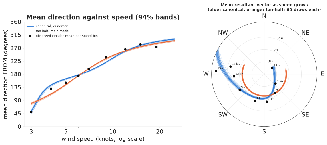
The observed mean resultant vectors (dots) trace a path that starts near the centre for the lightest winds (3 knots: from the northeast, but barely concentrated, $\bar R = 0.16$), swings through the southeast and south with $\bar R$ growing from 0.23 to 0.46, and ends in the west for the strongest winds ($\bar R$ 0.5-0.8). The tan-half link can only move the direction at a constant concentration - its spaghetti is an arc of a circle - so it overstates how concentrated light winds are and understates it for moderate ones. The canonical link moves the point freely in the plane and follows the path. Both sets of curves are tight: with 12,000 reports the uncertainty in the mean is small; the spread of individual winds around it (the grey cloud above) is large.
Two honest caveats. The reports are hourly and strongly autocorrelated, so LOO over hours treats 12,000 reports as more independent information than they are; Part D uses a held-out year as the stricter test. And speed and direction are both outcomes of the same weather: this is a description of the direction given the speed, not a causal effect of speed.
D. Direction on hour of day and season: circular predictors
The daily swing is the dominant signal. Hour of day and day of year are themselves circular predictors, and a circular predictor is the easy case: represent it by its harmonics $\cos(k\cdot 2\pi h/24), \sin(k\cdot 2\pi h/24)$, which are continuous across midnight and New Year. We use three daily harmonics, two annual harmonics and the products of the first two daily with the first annual harmonic (so the daily cycle can change with the season): 19 features including the intercept.
Three models for the direction, each with the features entering linearly (so each has $19 \times 2$ coefficients):
- von Mises, canonical link: $\eta(h, d) = F(h, d)\,B$, as in Part C.
- projected normal: a latent vector $z \sim N(F(h, d)\,B, I)$ whose angle is the direction. The mean vector can wander anywhere in the plane, including the origin, so there is no wrapping at all; the density has a closed form once the latent length is integrated out, $p(\theta) = \frac{1}{2\pi} e^{-|m|^2/2}\{1 + u\,\Phi(u)/\phi(u)\}$ with $u = m\cdot(\cos\theta, \sin\theta)$.
- a mixture of two regimes: an easterly regime (night drainage and morning flow) and a westerly regime (the sea breeze), each a von Mises whose natural parameters follow a smaller set of features (intercept, two daily and one annual harmonic), with the probability of the westerly regime following all 19 features through a logistic link.
Priors: normal(0, 2) on the intercepts and normal(0, 1) on the other coefficients. With harmonics in $[-1, 1]$, a prior draw of $\eta$ has a length of a few units: the implied concentrations at the training rows have a prior median of about 4 and a 90% range of about 1 to 8 - from "barely a preferred direction" to "a narrow sea breeze".
def features(df):
    h = TWO_PI * df.hour.to_numpy() / 24
    d = TWO_PI * df.doy.to_numpy()
    cols, names = [np.ones_like(h)], ["1"]
    for k in (1, 2, 3):
        cols += [np.cos(k * h), np.sin(k * h)]
        names += [f"cos{k}h", f"sin{k}h"]
    for k in (1, 2):
        cols += [np.cos(k * d), np.sin(k * d)]
        names += [f"cos{k}d", f"sin{k}d"]
    for k in (1, 2):
        for a, an in ((np.cos(k * h), f"cos{k}h"), (np.sin(k * h), f"sin{k}h")):
            for b, bn in ((np.cos(d), "cos1d"), (np.sin(d), "sin1d")):
                cols.append(a * b)
                names.append(f"{an}*{bn}")
    return np.column_stack(cols), names


F_tr, FEAT = features(train)
F_te, _ = features(test)
SMALL = [0, 1, 2, 3, 4, 7, 8]                              # 1, cos1h, sin1h, cos2h, sin2h, cos1d, sin1d
prior_sd = np.r_[2.0, np.ones(len(FEAT) - 1)]
coords = {"feat": FEAT, "comp": ["eta1", "eta2"], "sfeat": [FEAT[i] for i in SMALL],
          "regime": ["easterly", "westerly"]}

# prior predictive: implied concentration at the training rows
B_prior = rng.normal(0, prior_sd[None, :, None], size=(200, len(FEAT), 2))
kap_prior = np.hypot(*np.moveaxis(np.einsum("nf,sfc->snc", F_tr[:2000], B_prior), -1, 0))
print("prior concentration at training rows: quantiles 5/50/95% =", np.round(np.quantile(kap_prior, [0.05, 0.5, 0.95]), 2))

t0 = time.time()
with pm.Model(coords=coords) as m_vm:
    B = pm.Normal("B", 0, prior_sd[:, None], dims=("feat", "comp"))
    eta = pt.dot(F_tr, B)
    pm.Potential("ll", pt.sum(vm_lp(th, eta[:, 0], eta[:, 1])))
    idata_vm = pm.sample(random_seed=RANDOM_SEED, progressbar=False)
print(f"von Mises regression: {time.time() - t0:.0f} s")

t0 = time.time()
with pm.Model(coords=coords) as m_pn:
    B = pm.Normal("B", 0, prior_sd[:, None], dims=("feat", "comp"))
    m = pt.dot(F_tr, B)
    u = m[:, 0] * np.cos(th) + m[:, 1] * np.sin(th)
    pm.Potential("ll", pt.sum(-np.log(TWO_PI) - 0.5 * pt.sum(m ** 2, axis=1)
                              + pt.log1p(u * np.sqrt(np.pi / 2) * pt.erfcx(-u / np.sqrt(2)))))
    idata_pn = pm.sample(random_seed=RANDOM_SEED, progressbar=False)
print(f"projected normal regression: {time.time() - t0:.0f} s")

MU_PRIOR = wrap(np.deg2rad([90.0, 250.0]))                 # easterly from E, westerly from WSW
t0 = time.time()
with pm.Model(coords=coords) as m_mix:
    B0 = pm.Normal("B0", 2.0 * np.column_stack([np.cos(MU_PRIOR), np.sin(MU_PRIOR)]), 1.0, dims=("regime", "comp"))
    Bh = pm.Normal("Bh", 0, 1, shape=(2, len(SMALL) - 1, 2))
    Bc = pt.concatenate([B0[:, None, :], Bh], axis=1)      # regime x small feature x component
    e_e = pt.dot(F_tr[:, SMALL], Bc[0])
    e_w = pt.dot(F_tr[:, SMALL], Bc[1])
    g = pm.Normal("g", 0, np.r_[1.5, np.ones(len(FEAT) - 1)], dims="feat")
    z = pt.dot(F_tr, g)
    ll = pt.logaddexp(-pm.math.log1pexp(z) + vm_lp(th, e_e[:, 0], e_e[:, 1]),
                      -pm.math.log1pexp(-z) + vm_lp(th, e_w[:, 0], e_w[:, 1]))
    pm.Potential("ll", pt.sum(ll))
    idata_mix = pm.sample(random_seed=RANDOM_SEED, progressbar=False)
print(f"mixture of regimes: {time.time() - t0:.0f} s")

for name, idd, vs in (("von Mises", idata_vm, ["B"]), ("projected normal", idata_pn, ["B"]),
                      ("mixture", idata_mix, ["B0", "Bh", "g"])):
    s = pd.concat([az.summary(idd, var_names=[v], round_to=4) for v in vs])
    print(f"{name:17s} max r_hat {s.r_hat.max():.3f}, min bulk ESS {s.ess_bulk.min():.0f}, "
          f"divergences {int(idd.sample_stats['diverging'].sum())}, mean tree depth "
          f"{float(idd.sample_stats['depth'].mean()):.1f}, warm-up {idd.posterior.attrs.get('tuning_steps')}")
print(per_chain(idata_mix, []).round(1).to_string())
print("regime intercept directions per chain (deg):",
      np.round(np.rad2deg(np.arctan2(idata_mix.posterior["B0"].values[..., 1],
                                     idata_mix.posterior["B0"].values[..., 0]).mean(1)) % 360).tolist())
prior concentration at training rows: quantiles 5/50/95% = [1.03 3.96 8.23]
von Mises regression: 9 s
projected normal regression: 7 s
mixture of regimes: 68 s
von Mises         max r_hat 1.004, min bulk ESS 5664, divergences 0, mean tree depth 3.0, warm-up 400
projected normal  max r_hat 1.005, min bulk ESS 7265, divergences 0, mean tree depth 3.0, warm-up 400
mixture           max r_hat 1.006, min bulk ESS 733, divergences 0, mean tree depth 3.9, warm-up 400
         mean logp  divergences
chain 0   -15867.8            0
chain 1   -15867.4            0
chain 2   -15867.7            0
chain 3   -15867.4            0
regime intercept directions per chain (deg): [[127.0, 259.0], [127.0, 259.0], [127.0, 258.0], [127.0, 259.0]]
All three sample cleanly (the mixture takes longest). A mixture invites label switching - two chains could call the sea breeze "regime 1" and "regime 2" - and here the regimes are anchored by their priors on direction (east vs west-southwest), which is physically meaningful, and the chains agree on the regimes' directions. That has to be checked, not assumed: Part E shows what happens without such an anchor.
Which model predicts better?
We score each model twice: PSIS-LOO on the 2021-2022 training reports, and the log predictive density of every report of 2023, which none of the models saw. Autocorrelated hours make the LOO standard errors too small; for 2023 we compute the standard error of the difference from daily sums, so that correlated hours within a day count as one unit.
S_LL = 1000
draws = {
    "vm": az.extract(idata_vm, var_names=["B"], num_samples=S_LL, random_seed=1).transpose("sample", ...).values,
    "pn": az.extract(idata_pn, var_names=["B"], num_samples=S_LL, random_seed=1).transpose("sample", ...).values,
}
mx = az.extract(idata_mix, var_names=["B0", "Bh", "g"], num_samples=S_LL, random_seed=1)
draws["mix"] = (np.concatenate([mx["B0"].transpose("sample", ...).values[:, :, None, :],
                                mx["Bh"].transpose("sample", ...).values], axis=2),
                mx["g"].transpose("sample", ...).values)


def loglik(model, F, th_obs):
    if model == "vm":
        e = np.einsum("nf,sfc->snc", F, draws["vm"])
        return vm_logpdf(th_obs[None], e[..., 0], e[..., 1])
    if model == "pn":
        m = np.einsum("nf,sfc->snc", F, draws["pn"])
        return pn_logpdf(th_obs[None], m[..., 0], m[..., 1])
    Bc, g = draws["mix"]
    ee = np.einsum("nf,srfc->srnc", F[:, SMALL], Bc)
    z = np.einsum("nf,sf->sn", F, g)
    return np.logaddexp(-np.logaddexp(0, z) + vm_logpdf(th_obs[None], ee[:, 0, :, 0], ee[:, 0, :, 1]),
                        -np.logaddexp(0, -z) + vm_logpdf(th_obs[None], ee[:, 1, :, 0], ee[:, 1, :, 1]))


const_mu, const_R = mean_resultant(th)
const_k = A1inv(const_R)
loos, lpd_test = {}, {}
th_te = test.theta.to_numpy()
for mname in ("vm", "pn", "mix"):
    loos[mname] = loo_from_ll(loglik(mname, F_tr, th))
    lt = loglik(mname, F_te, th_te)
    lpd_test[mname] = special.logsumexp(lt, axis=0) - np.log(S_LL)
    del lt
lpd_test["one direction"] = vm_logpdf(th_te, const_k * np.cos(const_mu), const_k * np.sin(const_mu))
lpd_test["uniform"] = np.full(len(th_te), -np.log(TWO_PI))
names_long = {"vm": "von Mises (canonical)", "pn": "projected normal", "mix": "mixture of 2 regimes"}
print(az.compare({names_long[k]: v for k, v in loos.items()}, round_to=1).to_string())

day = test.lst.dt.dayofyear.to_numpy()
rows = []
for k, v in lpd_test.items():
    dd = pd.Series(v - lpd_test["mix"]).groupby(day).sum()
    rows.append({"model": names_long.get(k, k), "2023 log score per report": v.mean(),
                 "total vs mixture": v.sum() - lpd_test["mix"].sum(),
                 "se (by day)": dd.std() * np.sqrt(len(dd))})
print(pd.DataFrame(rows).set_index("model").round(3).to_string())
                       rank  elpd_diff   dse  p_worse diag_diff diag_elpd     p     elpd    se  weight
mixture of 2 regimes      0        0.0   0.0      NaN                      58.4 -15822.0  97.0     0.9
von Mises (canonical)     1    -1563.3  62.9      1.0                      37.6 -17385.3  79.6     0.0
projected normal          2    -1581.9  65.7      1.0                      38.9 -17403.9  84.1     0.1
                       2023 log score per report  total vs mixture  se (by day)
model
von Mises (canonical)                     -1.517          -916.131       74.947
projected normal                          -1.521          -939.988       80.661
mixture of 2 regimes                      -1.365             0.000        0.000
one direction                             -1.799         -2612.265      135.311
uniform                                   -1.838         -2848.531      148.217
Both scores agree on the ranking. In 2023, knowing the hour and season is worth 0.28 nats per report (von Mises regression) to 0.43 nats (mixture) over a single mean direction for the whole year, which in turn is only slightly better (0.04 nats) than knowing nothing. The von Mises and projected normal regressions are close (the von Mises slightly ahead). The mixture of regimes is clearly best, in LOO and in 2023, by many standard errors even with the day-level standard error. The rose diagrams in Part B suggested why; the posterior predictive check shows it directly.
Circular posterior predictive checks
For each 3-hour block, the bars are the observed rose diagram (30-degree bins); the lines and bands are the median and 90% range of the same rose diagram in 200 replicated datasets from each model.
def simulate(mname, F, n_rep, seed=1):
    r = np.random.default_rng(seed)
    if mname == "vm":
        e = np.einsum("nf,sfc->snc", F, draws["vm"][:n_rep])
        return r.vonmises(np.arctan2(e[..., 1], e[..., 0]), np.hypot(e[..., 0], e[..., 1]))
    Bc, g = draws["mix"]
    ee = np.einsum("nf,srfc->srnc", F[:, SMALL], Bc[:n_rep])
    west = r.random((n_rep, len(F))) < special.expit(np.einsum("nf,sf->sn", F, g[:n_rep]))
    e1 = np.where(west, ee[:, 1, :, 0], ee[:, 0, :, 0])
    e2 = np.where(west, ee[:, 1, :, 1], ee[:, 0, :, 1])
    return r.vonmises(np.arctan2(e2, e1), np.hypot(e1, e2))


N_REP = 200
rep = {m_: simulate(m_, F_tr, N_REP) for m_ in ("vm", "mix")}
bins12 = np.linspace(-np.pi / 12, TWO_PI - np.pi / 12, 13)
blk = (train.hour.to_numpy() // 3).astype(int)
fig, axes = plt.subplots(2, 4, figsize=(12, 6.6), subplot_kw={"projection": "polar"})
centres = bins12[:-1] + np.pi / 12
for b, ax in enumerate(axes.ravel()):
    sel = blk == b
    obs = np.histogram(np.mod(th[sel], TWO_PI), bins=bins12)[0] / sel.sum()
    ax.bar(centres, obs, width=TWO_PI / 12 * 0.92, color=LIGHT, edgecolor=MUTED, lw=0.5)
    for m_, c in (("vm", ORANGE), ("mix", BLUE)):
        h = np.array([np.histogram(np.mod(rep[m_][i, sel], TWO_PI), bins=bins12)[0] for i in range(N_REP)]) / sel.sum()
        lo, md, hi = np.quantile(h, [0.05, 0.5, 0.95], axis=0)
        cc = np.r_[centres, centres[0]]
        ax.fill_between(cc, np.r_[lo, lo[0]], np.r_[hi, hi[0]], color=c, alpha=0.35)
        ax.plot(cc, np.r_[md, md[0]], color=c, lw=1.5)
    compass(ax)
    ax.set_yticklabels([])
    ax.set_title(f"{3 * b:02d}:00-{3 * b + 3:02d}:00", fontsize=10)
fig.suptitle("Posterior predictive rose diagrams, 2021-2022 (grey bars: observed; orange: von Mises regression; "
             "blue: mixture of regimes; bands: 90% of 200 replicates)", fontsize=10);
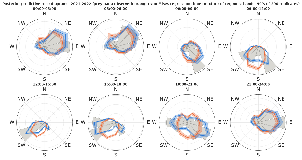
The single von Mises per hour and season cannot be in two places at once. In the 09:00-12:00 and 18:00-21:00 blocks, where the rose has two lobes, it puts much of its mass between them - in the south, where the wind rarely blows - and it is too flat in the afternoon. The mixture puts its mass on both lobes and is much closer everywhere. It is not perfect: the observed peaks are still sharper than its bands in several blocks (the SSE morning wind, the SW afternoon sea breeze, the easterly at night). Two regimes whose directions change smoothly with the hour are a simplification of real weather, and with 12,000 reports the check has the power to show it.
A rose diagram checks one hour block at a time. The probability integral transform (PIT) checks every report against its own predictive distribution: $u_i = P(\tilde\theta_i \text{ lies clockwise from the origin before } \theta_i)$, estimated from the replicates. On a circle the PIT needs an origin; for a correct model $u$ is uniform whatever the origin, but a misfit shows up differently from different origins, so we look at two. The 10-degree rounding would make the PIT lumpy, so each observed direction is jittered uniformly within its bin first.
jit = th + np.deg2rad(rng.uniform(-5, 5, n_tr))
fig, axes = plt.subplots(1, 2, figsize=(11, 3.6), sharey=True)
for ax, (org, olab) in zip(axes, ((0.0, "origin north"), (np.pi, "origin south"))):
    for m_, c, lab in (("vm", ORANGE, "von Mises regression"), ("mix", BLUE, "mixture of regimes")):
        u = (np.mod(rep[m_] - org, TWO_PI) < np.mod(jit - org, TWO_PI)[None]).mean(0)
        hist = np.histogram(u, bins=20, range=(0, 1))[0] / n_tr * 20
        ax.step(np.linspace(0, 1, 21), np.r_[hist, hist[-1]], where="post", color=c, lw=2, label=lab)
    band = 2 * np.sqrt(20 / n_tr)
    ax.axhspan(1 - band, 1 + band, color=LIGHT, alpha=0.8, label="±2 sd for a uniform PIT")
    ax.set(xlabel="PIT value", title=f"Circular PIT, {olab}")
axes[0].set_ylabel("density")
axes[0].legend(fontsize=8);
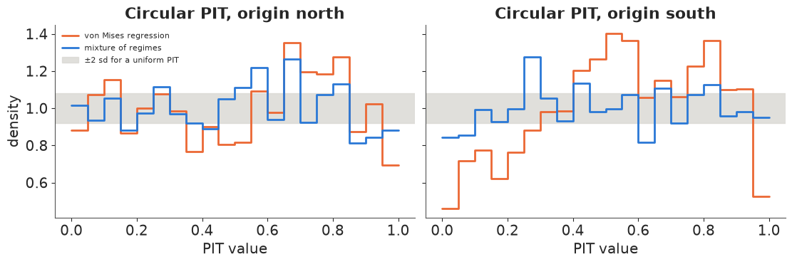
A calibrated model gives a flat line at 1. The von Mises regression's PIT is far from flat, most clearly from the southern origin (densities from 0.45 to 1.4). The mixture is much flatter from both origins but still leaves the ±2 sd band in several bins - the same residual misfit as in the rose diagrams. (The band assumes independent reports, which hourly winds are not, so it is too narrow.)
What the mixture says about hours and seasons
The mixture's gate - the probability that the sea-breeze regime is blowing - is a smooth function of hour and day of year. Its posterior mean and the width of its 94% interval:
hh = np.arange(0, 24, 0.5) + 0.25
dd = np.arange(0, 365, 7) + 3.5
H, D = np.meshgrid(hh, dd, indexing="ij")
grid_df = pd.DataFrame({"hour": H.ravel(), "doy": D.ravel() / 365.25})
F_g, _ = features(grid_df)
Bc_d, g_d = draws["mix"]
p_west = special.expit(np.einsum("nf,sf->sn", F_g, g_d[:400])).reshape(400, *H.shape)
lo, hi = np.quantile(p_west, [0.03, 0.97], axis=0)
fig, axes = plt.subplots(1, 2, figsize=(12, 4))
im = axes[0].pcolormesh(dd, hh, p_west.mean(0), cmap="Blues", vmin=0, vmax=1, shading="auto")
fig.colorbar(im, ax=axes[0], label="P(westerly regime)")
im2 = axes[1].pcolormesh(dd, hh, hi - lo, cmap="Greys", vmin=0, shading="auto")
fig.colorbar(im2, ax=axes[1], label="width of 94% interval")
month_starts = np.cumsum([0, 31, 28, 31, 30, 31, 30, 31, 31, 30, 31, 30])
for ax in axes:
    ax.set(xlabel="day of year", ylabel="hour (Pacific standard time)", yticks=range(0, 25, 3))
    ax.set_xticks(month_starts + 15)
    ax.set_xticklabels(list("JFMAMJJASOND"))
axes[0].set_title("Posterior mean probability of the sea-breeze regime")
axes[1].set_title("Uncertainty of that probability");
print("P(westerly) posterior mean, 15:00 in mid-January / mid-July: "
      f"{p_west.mean(0)[np.searchsorted(hh, 15), 2]:.2f} / {p_west.mean(0)[np.searchsorted(hh, 15), 28]:.2f}")
P(westerly) posterior mean, 15:00 in mid-January / mid-July: 0.71 / 0.87
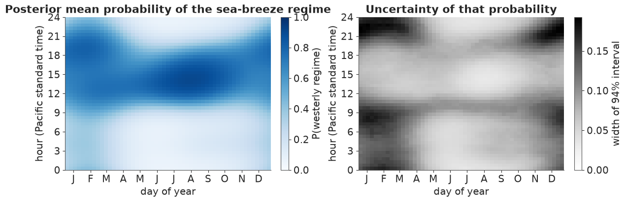
The westerly regime owns the early afternoon all year, most firmly in summer (close to 0.9 around 13:00-15:00 from June to September). In winter its peak is lower but it lasts later into the evening - until about 21:00 - and keeps a probability of 0.2-0.4 even at night, when westerlies probably come with passing weather systems rather than a sea breeze. The intervals are narrow in the afternoon and widest (0.15-0.19) on winter evenings and early mornings, where the two regimes' directions overlap and it is hard to tell which one a given wind belongs to.
A clock of wind arrows
How to show a direction that depends on a time of day, with its uncertainty? Below, each panel is a 24-hour clock. At each hour, arrows show the predicted mean resultant vector of the wind, drawn as the air moves (downwind, north up), with length proportional to $\bar R$: a long arrow means a steady wind, a short one a wind that could come from anywhere. Each of the 40 thin arrows per hour is one posterior draw, so the fan of arrows is the uncertainty in the mean vector.
def mix_mean_vector(F, Bc, g):
    """Predictive E[exp(i theta)] of the mixture for each draw and row."""
    ee = np.einsum("nf,srfc->srnc", F[:, SMALL], Bc)
    p = special.expit(np.einsum("nf,sf->sn", F, g))
    z = 0
    for r_, w_ in ((0, 1 - p), (1, p)):
        k = np.hypot(ee[:, r_, :, 0], ee[:, r_, :, 1])
        z = z + w_ * A1(k) * np.exp(1j * np.arctan2(ee[:, r_, :, 1], ee[:, r_, :, 0]))
    return z


hours = np.arange(0, 24, 1.0) + 0.5
fig, axes = plt.subplots(1, 2, figsize=(12, 6))
for ax, (doy, lab) in zip(axes, ((15, "mid-January"), (196, "mid-July"))):
    df_c = pd.DataFrame({"hour": hours, "doy": np.full(24, doy / 365.25)})
    Fc, _ = features(df_c)
    zc = mix_mean_vector(Fc, Bc_d[:40], g_d[:40])
    ax.add_patch(plt.Circle((0, 0), 1, fill=False, color=LIGHT, lw=1))
    for j, h in enumerate(hours):
        ang = TWO_PI * h / 24
        cx, cy = np.sin(ang), np.cos(ang)
        for s_ in range(40):
            d_from = np.angle(zc[s_, j])
            L = 0.6 * np.abs(zc[s_, j])
            dx, dy = -L * np.sin(d_from), -L * np.cos(d_from)          # downwind, north up
            ax.add_patch(FancyArrowPatch((cx - dx / 2, cy - dy / 2), (cx + dx / 2, cy + dy / 2),
                                         arrowstyle="-|>", mutation_scale=11, lw=0.8,
                                         color=BLUE if np.cos(d_from - np.deg2rad(250)) > 0 else ORANGE,
                                         alpha=0.25))
    for h in range(0, 24, 3):
        a = TWO_PI * h / 24
        ax.text(1.32 * np.sin(a), 1.32 * np.cos(a), f"{h:02d}:00", ha="center", va="center", fontsize=9, color=MUTED)
    ax.annotate("N", (0, 0.25), xytext=(0, -0.05), ha="center", arrowprops=dict(arrowstyle="->", color=MUTED), color=MUTED)
    ax.set(xlim=(-1.55, 1.55), ylim=(-1.55, 1.55), aspect="equal", title=f"{lab}: mean wind vector by hour")
    ax.axis("off")
fig.suptitle("Arrows point downwind (north up); length = mean resultant length; 40 posterior draws per hour. "
             "Blue: wind from the western half (sea breeze side), orange: from the eastern half", fontsize=10);
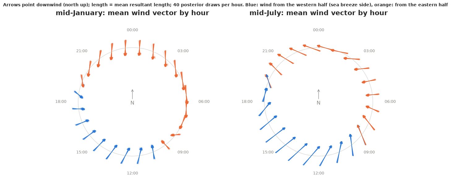
In January the night and early-morning arrows point south - air from the north-northeast draining out to sea - the late-morning arrows turn to point northwest (a southeasterly), and from about 11:00 to 19:00 the sea breeze pushes inland (arrows pointing northeast). In July the night flow comes from the east (arrows pointing west), and the sea-breeze phase runs from about 10:00 to 19:00 with longer arrows: a steadier wind. The shortest arrows are at the evening turnaround, not because the air is still (calms are excluded) but because the direction is least predictable. The fans of 40 draws are narrow: the mean vector is well determined, and the uncertainty that matters for a sailor is the spread of individual winds, which the arrow length encodes.
Circular intervals as arcs
For the direction of each regime at a given time, the natural uncertainty display is an arc on the compass: the shortest arc holding 94% of the posterior draws (a circular HDI). Below: the westerly regime at 15:00 and the easterly regime at 03:00, in mid-January and mid-July. Each arc sits at its own radius; the tick is the posterior circular mean.
fig = plt.figure(figsize=(6.5, 6.5))
ax = fig.add_subplot(projection="polar")
compass(ax)
arcs = []
for rad, (hour, doy, reg, lab, c) in enumerate(
        ((15, 15, 1, "westerly, 15:00, Jan", BLUE), (15, 196, 1, "westerly, 15:00, Jul", BLUE),
         (3, 15, 0, "easterly, 03:00, Jan", ORANGE), (3, 196, 0, "easterly, 03:00, Jul", ORANGE)), start=1):
    Fp, _ = features(pd.DataFrame({"hour": [hour], "doy": [doy / 365.25]}))
    ee = np.einsum("nf,sfc->snc", Fp[:, SMALL], Bc_d[:, reg])[:, 0]
    mu_draw = np.arctan2(ee[:, 1], ee[:, 0])
    lo_, hi_, cm_ = circ_hdi(mu_draw)
    arcs.append({"regime / time": lab, "mean (deg)": np.rad2deg(cm_) % 360,
                 "94% arc from": np.rad2deg(lo_) % 360, "to": np.rad2deg(hi_) % 360,
                 "width (deg)": np.rad2deg(hi_ - lo_), "kappa": np.median(np.hypot(ee[:, 0], ee[:, 1]))})
    tt = np.linspace(lo_, hi_, 50)
    r0 = 0.35 + 0.15 * rad
    ax.plot(tt, np.full_like(tt, r0), color=c, lw=6, solid_capstyle="butt", alpha=0.85)
    ax.plot([cm_, cm_], [r0 - 0.04, r0 + 0.04], color=INK, lw=1.5)
    ax.text(cm_ + 0.12, r0, lab, fontsize=8, va="center")
ax.set_ylim(0, 1.05)
ax.set_yticklabels([])
ax.set_title("94% circular HDIs of each regime's mean direction", fontsize=10)
print(pd.DataFrame(arcs).set_index("regime / time").round(1).to_string())
                      mean (deg)  94% arc from     to  width (deg)  kappa
regime / time
westerly, 15:00, Jan       255.2         253.3  257.2          3.9    4.0
westerly, 15:00, Jul       240.6         239.4  241.7          2.3    7.6
easterly, 03:00, Jan        29.4          25.7   33.3          7.5    3.2
easterly, 03:00, Jul        88.7          84.6   92.7          8.0    1.7
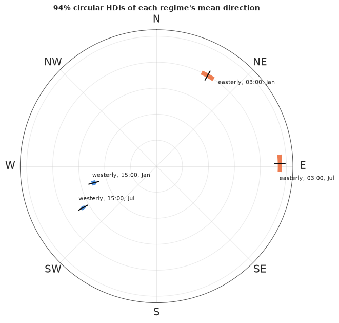
The arcs are only a few degrees wide. The regime's mean direction is known to within a few degrees; individual hours scatter around it with the concentration $\kappa$ in the last column (a von Mises with $\kappa = 5$ has an angular standard deviation of roughly 27 degrees). Both regimes change with the season by much more than their arcs: the afternoon westerly comes from about 255 degrees in January and 241 in July (and is twice as concentrated in July), and the night easterly from the north-northeast (about 30 degrees) in January but from due east in July. Note that an arc crossing north needs care: the HDI is computed on angles relative to the circular mean so it is never split at 0/360.
E. When is an ocelot about? Activity on the 24-hour circle
Camera traps photograph whatever walks past. The time stamps of many photographs of one species, taken on the same 24-hour circle, estimate its activity pattern: the density of activity over the day. Rowcliffe et al. (2014) deployed camera traps on Barro Colorado Island, Panama, in 2008; we use the ocelot and five of its potential prey.
Two caveats about such data, before any model. The records are photographs, not independent visits: one animal lingering in front of a camera can leave several records, which makes the data look more informative than they are (we use the records as distributed). And the times are clock times without dates. Animals follow the sun; at 9 degrees north sunrise and sunset move by well under an hour over the year, so clock time is a tolerable proxy here - far from the equator it is not.
data.describe("bci_camera_trap")
cam_all = data.load("bci_camera_trap")
SPECIES = ["ocelot", "agouti", "paca", "rat", "brocket", "peccary"]
cam = cam_all[cam_all.species.isin(SPECIES)].copy()
cam["th"] = TWO_PI * cam.time                    # 0 = midnight, pi = noon
xs = {s_: cam.th[cam.species == s_].to_numpy() for s_ in SPECIES}
print(pd.DataFrame({"records": {s_: len(v) for s_, v in xs.items()},
                    "mean time": {s_: f"{(np.rad2deg(mean_resultant(v)[0]) % 360) / 15:.1f} h" for s_, v in xs.items()},
                    "R": {s_: mean_resultant(v)[1] for s_, v in xs.items()}}).round(2).T.to_string())

fig, axes = plt.subplots(2, 3, figsize=(11, 7.4), subplot_kw={"projection": "polar"})
for ax, s_ in zip(axes.ravel(), SPECIES):
    cnt, edges = np.histogram(xs[s_], bins=24, range=(0, TWO_PI))
    ax.bar(edges[:-1] + np.pi / 24, cnt / cnt.sum(), width=TWO_PI / 24 * 0.9, color=BLUE if s_ == "ocelot" else ORANGE)
    clockface(ax)
    ax.set_yticklabels([])
    ax.set_title(f"{s_} ({len(xs[s_])} records)", fontsize=10)
fig.suptitle("Camera-trap records on Barro Colorado Island by hour of day (clock faces: midnight at the top)", fontsize=10);
bci_camera_trap: 17,820 camera-trap records from Barro Colorado Island, Panama, 2008: species (13: agouti, peccary, paca, rat, brocket, squirrel, coati, ocelot, tamandua, armadillo, opossum, mouse, tayra) and time (time of day as a fraction of 24 hours, to the minute; no dates).
  source: Rowcliffe, Kays, Kranstauber, Carbone & Jansen (2014), 'Activity level estimation data', figshare, doi:10.6084/m9.figshare.1160536 (CC BY 4.0), file BCItime.txt; data of Rowcliffe et al. (2014), 'Quantifying levels of animal activity using camera trap data', Methods in Ecology and Evolution 5:1170-1179. Also shipped as `BCItime` in the R package activity. CONVERTED from space- to comma-separated by tools/build_e81_circular.py - keep the cached file.
  url:    https://ndownloader.figshare.com/files/3219290
           ocelot  agouti    paca    rat brocket peccary
records       317   10292     999    893     816    2965
mean time  22.8 h  11.0 h  23.7 h  0.5 h   1.8 h  21.2 h
R            0.36    0.52    0.73   0.63    0.12    0.09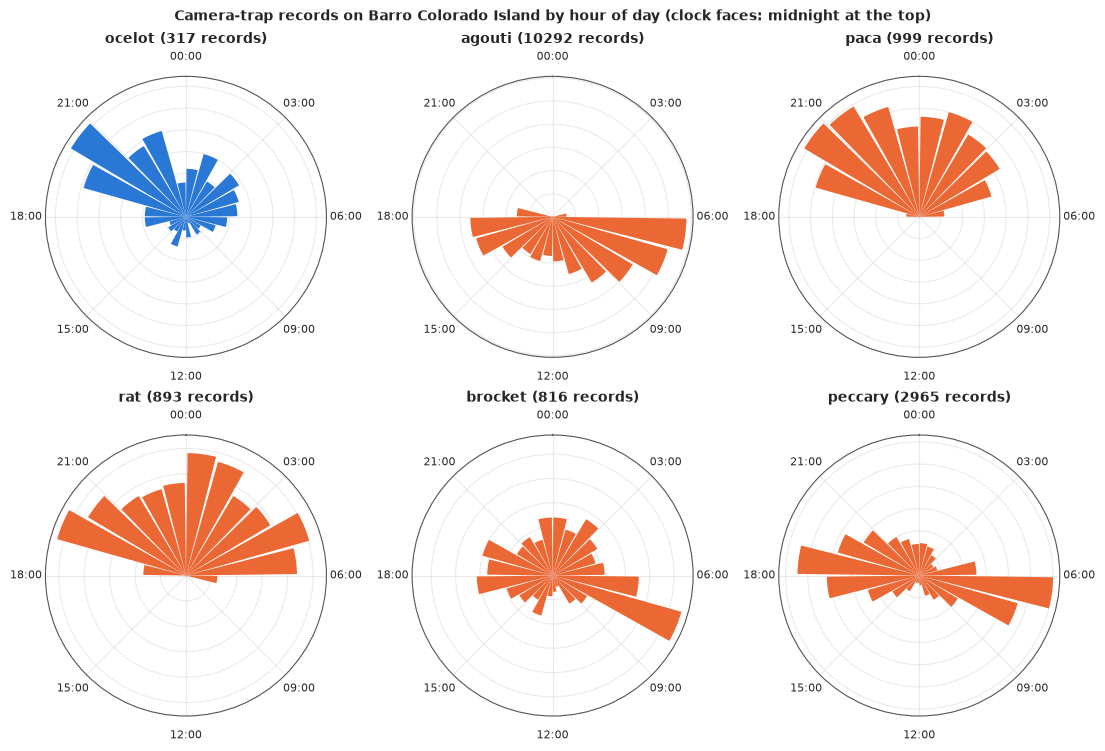
The ocelot is mostly nocturnal, with a peak in the evening (19:00-21:00) and few daytime records; the agouti is diurnal with two peaks, after dawn and before dusk; the paca and the spiny rat are nocturnal; the red brocket deer is about at all hours with a peak at dawn; the collared peccary is active by day with peaks at dawn and dusk. The mean times and $\bar R$ in the table are again poor summaries: the agouti's two peaks give a "mean time" of 11:00, when it is less active than at 07:00 or 17:00, and the peccary's two peaks nearly cancel ($\bar R$ = 0.09) to a meaningless mean time of 21:00.
A von Mises mixture, the obvious way - and what goes wrong
A flexible activity density is a mixture of von Mises distributions. Fitted the obvious way - means uniform on $(-\pi, \pi)$, where $\pm\pi$ is noon, concentrations and weights with standard priors - to the agouti's 10,292 records with two components:
def vm_mix_density(mu, kappa, w, at):
    """Density of a von Mises mixture on the grid `at`; parameters (..., K)."""
    return (w[..., None] * np.exp(kappa[..., None] * (np.cos(at - mu[..., None]) - 1))
            / (TWO_PI * special.i0e(kappa[..., None]))).sum(-2)


def max_rhat(arr):
    """Largest r_hat over the trailing dimensions of a (chain, draw, ...) array."""
    dims = ("chain", "draw") + tuple(f"d{i}" for i in range(arr.ndim - 2))
    return float(np.nanmax(az.rhat(xr.Dataset({"v": (dims, arr)}))["v"].values))


G = 256
cgrid = np.arange(G) * TWO_PI / G                    # clock grid, 0 = midnight
x_ag = wrap(xs["agouti"])
with pm.Model() as m_agouti_uniform:
    mu = pm.Uniform("mu", -np.pi, np.pi, shape=2)
    kappa = pm.Gamma("kappa", 2.0, 0.5, shape=2)
    w = pm.Dirichlet("w", np.ones(2))
    pm.Mixture("y", w=w, comp_dists=pm.VonMises.dist(mu=mu, kappa=kappa), observed=x_ag)
    idata_ag_u = pm.sample(random_seed=RANDOM_SEED, progressbar=False)
post = {v: idata_ag_u.posterior[v].values for v in ("mu", "kappa", "w")}
tab = pd.DataFrame({
    "peak times (h)": [", ".join(f"{(np.rad2deg(m_) % 360) / 15:.1f}" for m_ in mean_resultant(post["mu"][c], axis=0)[0])
                       for c in range(4)],
    "kappa": [np.round(post["kappa"][c].mean(0), 1).tolist() for c in range(4)],
    "weights": [np.round(post["w"][c].mean(0), 2).tolist() for c in range(4)],
    "mean logp": idata_ag_u.sample_stats["logp"].values.mean(1).round(1),
    "divergences": idata_ag_u.sample_stats["diverging"].values.sum(1)})
print(tab.to_string())
dens_u = vm_mix_density(post["mu"], post["kappa"], post["w"], cgrid)
print(f"max r_hat of the parameters: {max(max_rhat(post[v]) for v in post):.2f}; "
      f"max r_hat of the density on a 256-point grid: {max_rhat(dens_u):.2f}")
  peak times (h)        kappa       weights  mean logp  divergences
0      8.3, 15.7   [5.7, 4.2]  [0.58, 0.42]   -13168.7            0
1     17.3, 12.0  [30.9, 1.3]  [0.13, 0.87]   -15555.2            0
2      15.7, 8.3   [4.2, 5.7]  [0.43, 0.57]   -13168.7            0
3      8.3, 15.7   [5.7, 4.2]  [0.58, 0.42]   -13168.7            0
max r_hat of the parameters: 2.41; max r_hat of the density on a 256-point grid: 1.53
Two different things went wrong, and only one of them matters:
- Label switching. Some chains call the morning peak "component 1", others "component 2". That alone makes every parameter's $\hat R$ large, but it is harmless: the density is the same whatever the labels. The right check for anything label-invariant (the density, an overlap, an activity level) is $\hat R$ of that quantity itself.
- A chain stuck at the seam. One chain has a component pressed against $\pm\pi$ = noon (a peak time of 12.0 h), with a much lower log density: the wall of the uniform prior again, now inside a mixture. This one is not harmless - the density itself disagrees between chains ($\hat R$ of the density well above 1.01) - and again there are zero divergences.
The cure is the same as in Part C: give each component its natural parameters, $\eta_k = \kappa_k(\cos\mu_k, \sin\mu_k) \sim N(0, 3^2 I)$, so each component's mean is a point in the plane with no seam and its concentration is that point's distance from the origin. We fit two and three components to the ocelot and the agouti and check $\hat R$ both ways.
def fit_vm_mixture(x, K):
    with pm.Model() as m:
        eta = pm.Normal("eta", 0, 3, shape=(K, 2))
        pm.Deterministic("mu", pt.arctan2(eta[:, 1], eta[:, 0]))
        pm.Deterministic("kappa", pt.sqrt(pt.sum(eta ** 2, axis=1)))
        w = pm.Dirichlet("w", np.ones(K))
        pm.Mixture("y", w=w, comp_dists=pm.VonMises.dist(mu=m["mu"], kappa=m["kappa"]), observed=wrap(x))
        return pm.sample(random_seed=RANDOM_SEED, progressbar=False)


rows, loo_act = [], {s_: {} for s_ in ("ocelot", "agouti")}
for s_ in ("ocelot", "agouti"):
    for K in (2, 3):
        t0 = time.time()
        idd = fit_vm_mixture(xs[s_], K)
        p_ = {v: idd.posterior[v].values for v in ("mu", "kappa", "w")}
        rows.append({"species": s_, "components": K, "seconds": time.time() - t0,
                     "divergences": int(idd.sample_stats["diverging"].sum()),
                     "max r_hat, parameters": max(max_rhat(p_[v]) for v in p_),
                     "max r_hat, density": max_rhat(vm_mix_density(p_["mu"], p_["kappa"], p_["w"], cgrid))})
        ex = az.extract(idd, var_names=["mu", "kappa", "w"], num_samples=1000, random_seed=1)
        mu_, k_, w_ = (ex[v].transpose("sample", ...).values for v in ("mu", "kappa", "w"))
        ll = special.logsumexp(np.log(w_)[:, None, :] + k_[:, None, :] * (np.cos(xs[s_][None, :, None] - mu_[:, None, :]) - 1)
                               - np.log(TWO_PI * special.i0e(k_))[:, None, :], axis=2)
        loo_act[s_][f"von Mises mixture, K = {K}"] = loo_from_ll(ll)
        if s_ == "agouti" and K == 3:
            agouti_mix3 = (mu_, k_, w_)
        del idd, ll
print(pd.DataFrame(rows).round(3).to_string(index=False))
species  components  seconds  divergences  max r_hat, parameters  max r_hat, density
 ocelot           2    1.277            0                  1.004               1.003
 ocelot           3    1.846            0                  1.334               1.006
 agouti           2    6.480            0                  1.533               1.004
 agouti           3   15.382            0                  2.419               1.007
With natural parameters no chain is stuck and there are no divergences. The parameters still have $\hat R$ well above 1 for three components (and for the agouti with two) because the chains label the components differently, but the density agrees across chains ($\hat R \le 1.01$). We could impose an order on the components to stop the switching, but "ordered" on a circle is itself ambiguous (ordered from where?), and nothing we want to report depends on the labels.
A label-free alternative: the log-Fourier density
If the labels are a nuisance, use a model without labels. Any smooth positive density on the circle can be written as the exponential of a Fourier series:
$$\log f(\theta) = \sum_{k=1}^{K} \big(a_k\cos k\theta + b_k\sin k\theta\big) - \log Z(a, b).$$
The von Mises is the case $K = 1$; with more harmonics this is an exponential family whose sufficient statistics are the trigonometric moments $\sum_i \cos k\theta_i$, $\sum_i \sin k\theta_i$. So the log-likelihood of all 10,292 agouti records costs as much as that of one: $\sum_k (a_k C_k + b_k S_k) - n\log Z$. $Z$ is an integral of a smooth periodic function, for which the plain average over an equally spaced grid (256 points here) is accurate to many digits. We use $K = 16$ harmonics with a smoothness prior $a_k, b_k \sim N(0, (\tau/k)^2)$ - higher harmonics shrink harder - and a half-normal(2) prior on each species' $\tau$, all six species in one model.
KH = 16
kk = np.arange(1, KH + 1)
Cg, Sg = np.cos(np.outer(cgrid, kk)), np.sin(np.outer(cgrid, kk))
n_sp = np.array([len(xs[s_]) for s_ in SPECIES])
Csum = np.array([np.cos(np.outer(xs[s_], kk)).sum(0) for s_ in SPECIES])     # trigonometric moments
Ssum = np.array([np.sin(np.outer(xs[s_], kk)).sum(0) for s_ in SPECIES])
dth_g = TWO_PI / G
# check the grid integral: a von Mises with kappa = 18 (sharper than any activity peak here)
vm18 = np.exp(18 * (np.cos(cgrid) - 1))
print(f"grid normaliser vs exact for kappa = 18: {vm18.sum() * dth_g:.12f} vs {TWO_PI * special.i0e(18):.12f}")

t0 = time.time()
with pm.Model(coords={"species": SPECIES, "k": kk, "grid": np.arange(G)}) as m_fourier:
    tau = pm.HalfNormal("tau", 2.0, dims="species")
    za = pm.Normal("za", 0, 1, dims=("species", "k"))
    zb = pm.Normal("zb", 0, 1, dims=("species", "k"))
    a = pm.Deterministic("a", za * tau[:, None] / kk, dims=("species", "k"))
    b = pm.Deterministic("b", zb * tau[:, None] / kk, dims=("species", "k"))
    lg = pt.dot(a, Cg.T) + pt.dot(b, Sg.T)
    logZ = pt.logsumexp(lg, axis=1) + np.log(dth_g)
    pm.Potential("ll", pt.sum(a * Csum + b * Ssum) - pt.sum(n_sp * logZ))
    pm.Deterministic("f", pt.exp(lg - logZ[:, None]), dims=("species", "grid"))
    idata_f = pm.sample(random_seed=RANDOM_SEED, progressbar=False)
print(f"log-Fourier model, 6 species: {time.time() - t0:.0f} s; divergences "
      f"{int(idata_f.sample_stats['diverging'].sum())}; max r_hat of tau {az.rhat(idata_f, var_names=['tau'])['tau'].max().item():.3f}; "
      f"max r_hat of the densities {max_rhat(idata_f.posterior['f'].values):.3f}")

fd = az.extract(idata_f, var_names=["f"], num_samples=1000, random_seed=1).transpose("sample", ...).values   # S, species, G
Ad = az.extract(idata_f, var_names=["a"], num_samples=1000, random_seed=1).transpose("sample", ...).values
Bd = az.extract(idata_f, var_names=["b"], num_samples=1000, random_seed=1).transpose("sample", ...).values
logZd = np.log(np.exp(Ad @ Cg.T + Bd @ Sg.T).sum(-1) * dth_g)
for j, s_ in enumerate(SPECIES):
    if s_ in loo_act:
        x = xs[s_]
        ll = Ad[:, j] @ np.cos(np.outer(x, kk)).T + Bd[:, j] @ np.sin(np.outer(x, kk)).T - logZd[:, j:j + 1]
        loo_act[s_][f"log-Fourier, K = {KH}"] = loo_from_ll(ll)
for s_ in loo_act:
    print(f"--- {s_}")
    print(az.compare(loo_act[s_], round_to=1)[["rank", "elpd", "elpd_diff", "dse", "p"]].to_string())
grid normaliser vs exact for kappa = 18: 0.595057202578 vs 0.595057202578
log-Fourier model, 6 species: 5 s; divergences 0; max r_hat of tau 1.003; max r_hat of the densities 1.005
--- ocelot
                          rank   elpd  elpd_diff  dse     p
von Mises mixture, K = 3     0 -526.4        0.0  0.0   6.9
von Mises mixture, K = 2     1 -527.5       -1.1  2.1   4.3
log-Fourier, K = 16          2 -528.4       -2.0  1.6  12.3
--- agouti
                          rank     elpd  elpd_diff   dse     p
log-Fourier, K = 16          0 -11928.2        0.0   0.0  26.8
von Mises mixture, K = 3     1 -12485.4     -557.1  28.6  12.9
von Mises mixture, K = 2     2 -13165.8    -1237.6  41.3   6.4
The log-Fourier model samples all six species at once in a few seconds, with no divergences and no labels to switch. For the ocelot (317 records) all three models are within 2 nats of each other: there is not enough information to separate them. For the agouti the log-Fourier density beats the three-component mixture by about 560 ± 30 nats: with 10,000 records the agouti's day has more structure than three von Mises bumps can hold (the peaks are not quite von Mises-shaped, and there is detail in between). A mixture would need more components - and more label switching - to catch up. The log-Fourier prior is still a smoothing choice (how fast $\tau/k$ shrinks the high harmonics), which matters for one of the quantities below. We use it for all species from here on.
How much does the ocelot's day overlap with its prey's?
The coefficient of overlap between two densities is the area under the lower of the two,
$$\Delta = \int_0^{2\pi} \min\{f_1(\theta), f_2(\theta)\}\,d\theta \in [0, 1],$$
1 for identical activity patterns and 0 for animals that are never about at the same time. Each posterior draw of the two densities gives a draw of $\Delta$. The usual estimator in ecology (Ridout & Linkie 2009, in the R package overlap) plugs in von Mises kernel density estimates, with the bandwidth from a rule of thumb, and gets intervals by bootstrap. We re-implement its $\hat\Delta_4$ (recommended for samples above about 75) in NumPy: the same bandwidth rule (a von Mises concentration estimated from the first three trigonometric moments), densities on a 512-point grid, and a plain percentile bootstrap over records (the package's own intervals use a smoothed bootstrap and a bias adjustment, so ours are only indicative).
def overlap_bandwidth(x, kmax=3):
    """Kernel concentration of the overlap package's rule (Ridout & Linkie 2009)."""
    m_ = np.arctan2(np.sin(x).sum(), np.cos(x).sum())
    est = []
    for k in range(1, kmax + 1):
        tm = np.hypot(np.sin(k * (x - m_)).mean(), np.cos(k * (x - m_)).mean())
        fk = lambda kap: special.ive(k, kap) / special.ive(0, kap) - tm
        est.append(brentq(fk, 1e-4, 345) if fk(1e-4) * fk(345) <= 0 else 0.0)
    kh = max(est)
    return (3 * len(x) * kh ** 2 * special.ive(2, 2 * kh) * np.exp(2 * kh)
            / (4 * np.sqrt(np.pi) * (special.ive(0, kh) * np.exp(kh)) ** 2)) ** 0.4


kgrid = np.arange(512) * TWO_PI / 512


def kernel_density(x, nu):
    """von Mises kernel density of x (radians) on kgrid, concentration nu, computed in chunks."""
    out = np.zeros(len(kgrid))
    for i in range(0, len(x), 2000):
        out += np.exp(nu * (np.cos(kgrid[:, None] - x[None, i:i + 2000]) - 1)).sum(1)
    return out / (len(x) * TWO_PI * special.ive(0, nu))


def interp_circ(dens, x):
    return np.interp(np.mod(x, TWO_PI), np.r_[kgrid, TWO_PI], np.r_[dens, dens[0]])


def dhat4(x, y):
    fx, fy = kernel_density(x, overlap_bandwidth(x)), kernel_density(y, overlap_bandwidth(y))
    return 0.5 * (np.minimum(1, interp_circ(fy, x) / interp_circ(fx, x)).mean()
                  + np.minimum(1, interp_circ(fx, y) / interp_circ(fy, y)).mean())


# prior predictive of Delta: two independent draws of the log-Fourier prior
n_pr = 2000
tau_pr = np.abs(rng.normal(0, 2, size=(n_pr, 2)))
a_pr = rng.normal(size=(n_pr, 2, KH)) * tau_pr[..., None] / kk
b_pr = rng.normal(size=(n_pr, 2, KH)) * tau_pr[..., None] / kk
lg_pr = a_pr @ Cg.T + b_pr @ Sg.T
f_pr = np.exp(lg_pr - special.logsumexp(lg_pr, axis=-1, keepdims=True)) / dth_g
delta_prior = np.minimum(f_pr[:, 0], f_pr[:, 1]).sum(-1) * dth_g

rng_b = np.random.default_rng(RANDOM_SEED)
N_BOOT = 200
ov_rows, delta_post = [], {}
for j, s_ in enumerate(SPECIES[1:], start=1):
    d_post = np.minimum(fd[:, 0], fd[:, j]).sum(-1) * dth_g
    delta_post[s_] = d_post
    x, y = xs["ocelot"], xs[s_]
    boot = np.array([dhat4(rng_b.choice(x, len(x)), rng_b.choice(y, len(y))) for _ in range(N_BOOT)])
    lo_, hi_ = np.quantile(d_post, [0.03, 0.97])
    ov_rows.append({"prey": s_, "posterior median": np.median(d_post), "94% from": lo_, "to": hi_,
                    "kernel Dhat4": dhat4(x, y), "bootstrap 3%": np.quantile(boot, 0.03),
                    "bootstrap 97%": np.quantile(boot, 0.97)})
ov = pd.DataFrame(ov_rows).set_index("prey")
print(ov.round(3).to_string())
print(f"prior of Delta between two independent prior densities: median {np.median(delta_prior):.2f}, "
      f"94% interval {np.quantile(delta_prior, 0.03):.2f}-{np.quantile(delta_prior, 0.97):.2f}")
         posterior median  94% from     to  kernel Dhat4  bootstrap 3%  bootstrap 97%
prey
agouti              0.303     0.257  0.350         0.300         0.259          0.338
paca                0.662     0.615  0.708         0.703         0.648          0.741
rat                 0.701     0.655  0.747         0.747         0.696          0.778
brocket             0.750     0.697  0.799         0.772         0.707          0.807
peccary             0.655     0.611  0.701         0.667         0.624          0.706
prior of Delta between two independent prior densities: median 0.30, 94% interval 0.02-0.82
hrs = cgrid / TWO_PI * 24
fig, axes = plt.subplots(2, 3, figsize=(13, 7))
for ax, s_ in zip(axes.ravel(), SPECIES[1:]):
    j = SPECIES.index(s_)
    m_oc, m_pr = fd[:, 0].mean(0) * TWO_PI / 24, fd[:, j].mean(0) * TWO_PI / 24     # per hour
    ax.fill_between(hrs, np.minimum(m_oc, m_pr), color=LIGHT, label="overlap (posterior means)")
    for arr, c, lab in ((fd[:, 0], BLUE, "ocelot"), (fd[:, j], ORANGE, s_)):
        lo_, hi_ = np.quantile(arr * TWO_PI / 24, [0.03, 0.97], axis=0)
        ax.fill_between(hrs, lo_, hi_, color=c, alpha=0.35)
        ax.plot(hrs, arr.mean(0) * TWO_PI / 24, color=c, lw=1.8, label=lab)
    r_ = ov.loc[s_]
    ax.set_title(f"ocelot vs {s_}: Delta = {r_['posterior median']:.2f} ({r_['94% from']:.2f}-{r_['to']:.2f})", fontsize=10)
    ax.set(xticks=range(0, 25, 6), xlim=(0, 24), ylim=(0, 0.16))
    ax.legend(fontsize=7, loc="upper center")
ax = axes.ravel()[-1]
ypos = np.arange(len(ov))[::-1]
for yy, (s_, r_) in zip(ypos, ov.iterrows()):
    ax.plot([r_["94% from"], r_["to"]], [yy + 0.12] * 2, color=BLUE, lw=4, solid_capstyle="butt")
    ax.plot(r_["posterior median"], yy + 0.12, "o", color=INK, ms=4)
    ax.plot([r_["bootstrap 3%"], r_["bootstrap 97%"]], [yy - 0.12] * 2, color=ORANGE, lw=4, solid_capstyle="butt")
    ax.plot(r_["kernel Dhat4"], yy - 0.12, "o", color=INK, ms=4)
ax.axvspan(np.quantile(delta_prior, 0.03), np.quantile(delta_prior, 0.97), color=LIGHT, alpha=0.6, zorder=0)
ax.set(yticks=ypos, yticklabels=ov.index, xlim=(0, 1), xlabel="coefficient of overlap with the ocelot",
       xticks=np.arange(0, 1.01, 0.2))
ax.set_title("Delta: Bayesian 94% (blue), kernel + bootstrap (orange);\ngrey: 94% prior range", fontsize=9)
for ax in axes[1, :2]:
    ax.set_xlabel("hour of day")
for ax in axes[:, 0]:
    ax.set_ylabel("activity density (per hour)")
fig.suptitle("Overlap of daily activity: ocelot (blue) against each prey (orange), 94% posterior bands", fontsize=11);
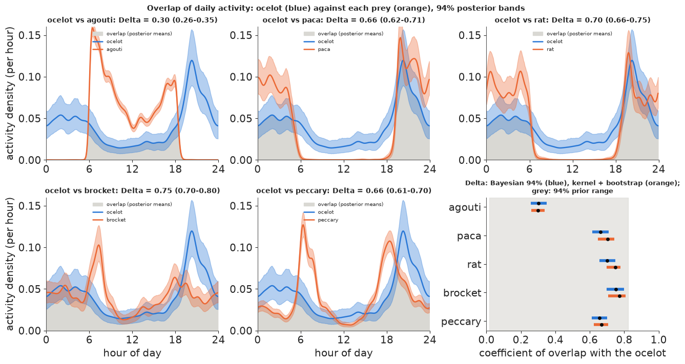
Reading the panels:
- The ocelot and the agouti overlap least (0.30): the agouti's two daytime peaks sit where the ocelot is quiet, and what overlap there is comes around dawn and dusk.
- The overlap is largest with the brocket (0.75), which is about at all hours, and with the nocturnal spiny rat (0.70) and paca (0.66); the day-active peccary overlaps about as much as the paca (0.66) because the ocelot's evening peak meets its dusk peak.
- The Bayesian and kernel estimates tell the same story. For the agouti they agree (0.30); for the other prey the posterior medians are 0.01-0.05 below the kernel $\hat\Delta_4$, and the posterior intervals are about as wide as the bootstrap intervals (0.08-0.10). The difference is smoothing: the kernel rule of thumb and our smoothness prior are different amounts of smoothing, and smoother densities overlap more. Neither is "the truth"; the Bayesian version at least makes the smoothing an explicit, checkable prior. The prior itself says little about $\Delta$: two independent draws from it overlap by anything from 0.02 to 0.82 (grey), so the data, not the prior, set these intervals.
The same overlap on a clock face, for the pair with the least and one with the most overlap:
fig, axes = plt.subplots(1, 2, figsize=(11, 5.4), subplot_kw={"projection": "polar"})
for ax, s_ in zip(axes, ("agouti", "paca")):
    j = SPECIES.index(s_)
    clockface(ax)
    th_c = np.r_[cgrid, cgrid[0]]
    m_oc, m_pr = fd[:, 0].mean(0), fd[:, j].mean(0)
    ax.fill_between(th_c, 0, np.r_[np.minimum(m_oc, m_pr), min(m_oc[0], m_pr[0])], color=LIGHT, lw=0)
    for arr, c, lab in ((fd[:, 0], BLUE, "ocelot"), (fd[:, j], ORANGE, s_)):
        lo_, hi_ = np.quantile(arr, [0.03, 0.97], axis=0)
        ax.fill_between(th_c, np.r_[lo_, lo_[0]], np.r_[hi_, hi_[0]], color=c, alpha=0.4)
        ax.plot(th_c, np.r_[arr.mean(0), arr.mean(0)[0]], color=c, lw=1.5, label=lab)
    ax.set_yticklabels([])
    ax.legend(loc="lower left", bbox_to_anchor=(-0.1, -0.12), fontsize=8)
    ax.set_title(f"ocelot and {s_}: Delta = {ov.loc[s_, 'posterior median']:.2f}", fontsize=10)
fig.suptitle("Activity densities on the 24-hour clock (bands: 94%; grey: the shared area)", fontsize=10);
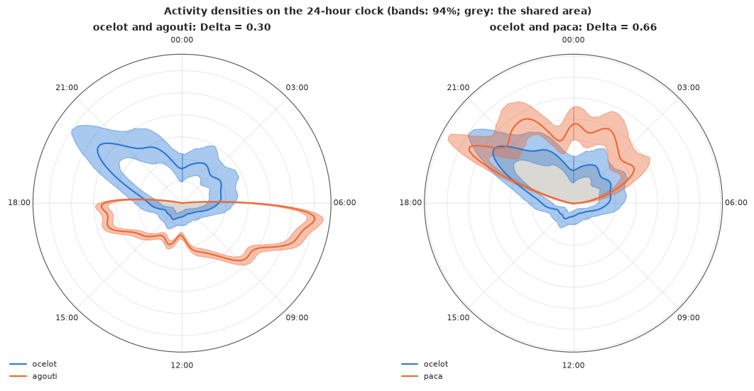
Activity level
Rowcliffe et al. (2014) turned the same curves into an estimate of the fraction of the day an animal is active: if at the peak of the activity curve the whole population is active, then the activity level is the ratio of the mean to the maximum of the density, $1 / (2\pi \max_\theta f(\theta))$. Each posterior draw gives one value. This is the quantity mentioned above that depends on the height of the peak, which is exactly what a smoothing prior (or a kernel bandwidth) controls.
act = 1 / (TWO_PI * fd.max(-1))
act_tab = pd.DataFrame({"median": np.median(act, 0), "94% from": np.quantile(act, 0.03, 0),
                        "to": np.quantile(act, 0.97, 0)}, index=SPECIES)
print(act_tab.round(3).to_string())
f_mix3 = vm_mix_density(*agouti_mix3, cgrid)
act_mix3 = 1 / (TWO_PI * f_mix3.max(-1))
print(f"agouti from the 3-component mixture: median {np.median(act_mix3):.3f} "
      f"(94%: {np.quantile(act_mix3, 0.03):.3f}-{np.quantile(act_mix3, 0.97):.3f}); overlap with the ocelot "
      f"{np.median(np.minimum(fd[:, 0], f_mix3).sum(-1) * dth_g):.3f}")
print(f"total run time {time.time() - T_START:.0f} s")
         median  94% from     to
ocelot    0.338     0.257  0.433
agouti    0.262     0.247  0.278
paca      0.279     0.232  0.323
rat       0.314     0.263  0.366
brocket   0.400     0.327  0.484
peccary   0.326     0.292  0.364
agouti from the 3-component mixture: median 0.255 (94%: 0.246-0.264); overlap with the ocelot 0.332
total run time 187 s
The ocelot is active about a third of the day (with a wide interval, 0.26-0.43, from 317 records), the agouti about a quarter. For the agouti the three-component mixture gives almost the same activity level (0.255 against 0.262) and overlap with the ocelot (0.33 against 0.30): here the choice of density model moves the answers by less than their uncertainty, although LOO clearly separated the models. That need not hold for a smaller sample, where the smoothing prior decides how high a peak may be. And the activity level assumes a fully active population at the peak, which camera times alone cannot check.
Summary
- Angles need vector averages. The arithmetic mean of wind directions fell between 169 and 209 degrees in every month; the circular mean moved from 110 to 275 degrees, and in December and January its mean resultant length was 0.02-0.04, i.e. no meaningful mean direction at all. Always report $\bar R$ with a mean direction, and remember that $\bar R$ is biased upwards in small samples (the "patternless" Oklahoma earthquakes gave 0.02, against 0.016 expected by chance).
- The von Mises is an exponential family - use it. In natural parameters $\eta = \kappa(\cos\mu, \sin\mu)$ the log-likelihood is concave. A regression with a canonical link (linear predictors for $\eta$) has a single mode, no walls and no wrapping, sampled cleanly every time, and fitted the direction-speed relation better than the tan-half link (by about 240 nats of LOO).
- Two traps give zero divergences. A uniform prior on an angle puts a wall at $\pm\pi$ (a chain was pinned there, $\hat R$ 2.4); the tan-half link has a genuine second mode where it becomes a step. Only $\hat R$ and per-chain summaries show them. The same wall broke an activity mixture (a chain stuck at "noon").
- Circular predictors are easy: use harmonics. Hour of day and day of year entered as cosines and sines. A mixture of two wind regimes with time-dependent gates beat the single von Mises and the projected normal regressions by about 1,560 nats of LOO and by 916 ± 75 nats on the held-out year 2023; rose diagrams with predictive bands and circular PIT showed why (two lobes at the transition hours) and what still misfits (peaks sharper than the model).
- Label switching is a diagnostic problem, not an inferential one when the target is label-invariant: check $\hat R$ on the density. A log-Fourier density fitted through its trigonometric moments has no labels at all, fits six species in seconds and beat a three-component mixture for the agouti by about 560 nats of LOO; its smoothing prior is still a choice to check.
- Overlap with honest uncertainty. The ocelot's activity overlapped least with the diurnal agouti (Delta 0.30) and most with the brocket, spiny rat and paca (0.66-0.75). Posterior intervals matched the bootstrap in width and sat 0-0.05 below the kernel estimate - a smoothing difference, made explicit by the prior.
Try it yourself
- Use the speed. The projected normal treats the direction as the angle of a latent vector - and for wind the vector exists: $(u, v) = -\text{speed}\,(\sin d, \cos d)$ for a wind from direction $d$. Model the observed wind vector with a bivariate normal (or a bivariate t) whose mean depends on hour and season, derive the implied distribution of the direction, and compare its 2023 log score for the direction with the mixture's. What happens to the calms?
- Wrapped Cauchy regimes. Replace the von Mises components of the wind mixture by wrapped Cauchy components (mean direction as atan2 of a linear predictor, $\rho$ through a logistic link). Heavier tails might absorb the stray directions that made the von Mises regimes too wide. Do LOO and the rose diagrams agree?
- Smoothing and activity levels. Refit the log-Fourier model with a slower-decaying prior ($\tau/\sqrt{k}$) or more harmonics, and recompute the activity level of the agouti and its overlap with the ocelot. Then compute both from the three-component mixture draws. How much of the difference between methods is smoothing, and which answer would you report to an ecologist?