The question
Fine particles in the air, PM2.5, are measured at regulatory monitors, and their three-year means decide whether an area meets the US annual standard of 9.0 µg/m³. About 1,000 sites in the contiguous US have usable daily data for 2023-2025. Four in five counties have none, and those counties hold about 100 million people.
Suppose a state air-monitoring planner, working with an EPA regional office, can fund a fixed number of new monitors and asks three things: which sites, how many are worth funding, and what would we be buying? The answer most people reach for is "put them where we are most uncertain". This notebook tests that answer and finds it wrong.
The idea that replaces it is preposterior analysis (Raiffa & Schlaifer 1961): before buying a measurement, work out how each reading it might give would change the decision, and how much better the decision gets on average. That gain is the expected value of sample information, and a very uncertain place can still offer no reading that would change what we do. Choosing sensor sites on a Gaussian process has a literature of its own (Krause, Singh & Guestrin 2008), which also supplies the greedy search we use to choose many sites at once.
What a wrong call means here. A county with no monitor has no legal call that could be wrong, so our loss is on exposure: the true 2023-2025 mean of the smooth regional field at a county's population centre, against the standard. Design values round to 0.1, so "above 9.0" means at least 9.05. A wrong call is our best estimate sitting on the other side of 9.05 from the truth, and a site is scored by the people moved from a wrong call to a right one. Dollars do not enter: we have no sourced cost for a monitor. Taking the smooth field as the truth leaves out the local difference a single site shows, and section 4 shows how much that choice matters.
No new monitor can help the current round: designations rest on 2023-2025 data and are due by 6 February 2027 under a court order now on appeal, and the standard itself is before the Supreme Court. We take 9.0 as given. A monitor running by 2028 first reports a three-year mean for 2028-2030, so the value we compute is a what-if: what a reading of the 2023-2025 field would have been worth. A real reading covers a later window, so the value runs somewhat high; section 7 sizes the gap.
We work on one 19-state crop of the Midwest, Ohio Valley, Plains and Rockies, with one model of the annual means, sized for 2 cores and under 3 GB. Nothing here speaks for the coasts, California or the Southeast. Sampling this dense model is not bit-reproducible even at a fixed seed, so your printed numbers will differ a little; where the text gives a range, it spans several builds of the notebook.
The plan
- The network, and what the raw files hide
- The model, on a map
- Can the map see what it has not measured?
- Which calls are close?
- Uncertainty is not value
- Choosing twenty sites
- How many monitors?
- Whose objective, which standard, which sites?
- The band
import os

for name in ("OPENBLAS_NUM_THREADS", "OMP_NUM_THREADS", "MKL_NUM_THREADS"):
    os.environ.setdefault(name, "1")  # before NumPy: one BLAS thread per chain

import contextlib
import gc
import json
import logging
import sys
import time
from concurrent.futures import ThreadPoolExecutor
from pathlib import Path

import arviz as az
import matplotlib.patheffects as pe
import matplotlib.pyplot as plt
import numpy as np
import pandas as pd
import pymc as pm
import pytensor
import pytensor.tensor as pt
from matplotlib.collections import LineCollection, PolyCollection
from matplotlib.colors import LinearSegmentedColormap, LogNorm, Normalize, TwoSlopeNorm
from matplotlib.ticker import NullFormatter
from scipy import linalg
from scipy.special import logsumexp, ndtr, ndtri

from pymc_challenges import data
from pymc_challenges.bigrun import PreflightError, banner, estimated, git_hash, measured

# ArviZ leaves a lazy stub under "jax", and Matplotlib's first plot tests `sys.modules.get("jax")`, which
# would import all of JAX for nothing. Nothing here uses JAX, so the stub goes.
sys.modules.pop("jax", None)

RANDOM_SEED = 89
rng = np.random.default_rng(RANDOM_SEED)
az.style.use("arviz-variat")
logging.getLogger("pymc").setLevel(logging.WARNING)

LEVEL = os.environ.get("PYMC_CHALLENGES_RUN", "").strip().lower() or "small"
if LEVEL != "small":
    raise PreflightError(f"PYMC_CHALLENGES_RUN={LEVEL!r}: E89 has one level, small. No national fit has "
                         "been run and no script exists for one, so there is nothing to replay or scale up.")
assert pytensor.config.floatX == "float64", "the annual path is float64"

CORES = len(os.sched_getaffinity(0)) if hasattr(os, "sched_getaffinity") else os.cpu_count()
CHAINS_AT_ONCE = min(4, CORES)
WORKERS = min(4, CORES)
LINE = 9.05  # the annual standard: design values round to 0.1
UG = "µg/m³"
METHODS = ("T640", "BAM", "other")  # FRM is the reference, so predictions are FRM-equivalent
YEARS = (2023, 2024, 2025)
SCALES = ("NEIGHBORHOOD", "URBAN SCALE", "REGIONAL SCALE", "MIDDLE SCALE", "MICROSCALE", "unknown")
PRIOR_ELL, PRIOR_ETA, PRIOR_TAU = (np.log(400.0), 0.6), (np.log(0.2), 0.6), (np.log(0.1), 0.6)
ABOVE, BELOW, PICK, MUTED = "#b2182b", "#2166ac", "#e66101", "#8a8a8a"
CLOSE_CALL = LinearSegmentedColormap.from_list(  # darkest where the call is closest, pale where it is settled
    "close_call", [(0, "#e6edf2"), (0.25, "#6baed6"), (0.4999, "#08306b"), (0.5001, "#67000d"), (0.75, "#fb6a4a"),
                   (1, "#fde8e2")])
PRICE = {}


@contextlib.contextmanager
def stage(name):
    """Add the time spent in this block to the price table printed at the end."""
    start = time.perf_counter()
    yield
    PRICE[name] = PRICE.get(name, 0.0) + time.perf_counter() - start


print(f"{CORES} cores here: {CHAINS_AT_ONCE} chains at once, {WORKERS} scoring threads")
2 cores here: 2 chains at once, 2 scoring threads
banner(wall_time=measured(16, "min on 2 cores, build of 2026-11-02"),
       peak_ram=measured(2.6, "GB, whole process tree"),
       peak_vram=measured(0, "GB: no GPU, and JAX never executes"),
       disk=measured(3.7, "MB in data/: 0.6 of tables and the 3.1 county geojson"),
       download=measured(0, "MB: the tables are built by tools/build_e89_data.py"),
       precision=measured("float64", ""),
       chains=measured(4, "chains, 500 draws, 3 fits"),
       hardware=measured("Ryzen 5950X, on 2 cores", ""),
       build_date=measured("2026-11-02", ""),
       git_hash=measured(git_hash() or "unknown", ""),
       smaller_machine=estimated("this is the small problem: no larger level exists", ""))
| Value | Status | |
|---|---|---|
| Wall time | 16 min on 2 cores, build of 2026-11-02 | measured |
| Peak RAM | 2.6 GB, whole process tree | measured |
| Peak VRAM | 0 GB: no GPU, and JAX never executes | measured |
| Disk | 3.7 MB in data/: 0.6 of tables and the 3.1 county geojson | measured |
| Download size | 0 MB: the tables are built by tools/build_e89_data.py | measured |
| Precision | float64 | measured |
| Chains | 4 chains, 500 draws, 3 fits | measured |
| Hardware | Ryzen 5950X, on 2 cores | measured |
| Build date | 2026-11-02 | measured |
| Git hash | ec322cc945d5-dirty | measured |
| On a smaller machine | this is the small problem: no larger level exists | estimated |
1 · The network, and what the raw files hide
Two tables, built by tools/build_e89_data.py from EPA's daily files and Census counts, hold one
row per site (its 2023-2025 mean, days and years reported, instruments and measurement scale) and
one row per county (population, population centre, and whether it has a monitor). The first map
shades the empty counties of the contiguous US by population and outlines our crop.
data.describe("e89_sites")
data.describe("e89_counties")
sites = data.load("e89_sites")
sites = sites[sites["conus"]].reset_index(drop=True)
sites["scale"] = sites["scale"].fillna("unknown")
counties = data.load("e89_counties")
checks = json.loads(data.path("e89_checks").read_text())
crop_sites = sites[sites["small_crop"]].reset_index(drop=True)
table = counties[counties["small_crop"]].reset_index(drop=True)
population = table["population"].to_numpy(float)
candidates = np.flatnonzero(~table["monitored"] & ~table["registered_only"])

empty = ~counties["monitored"]
print(f"Contiguous US: {len(sites):,} sites, {len(counties):,} counties, {empty.sum():,} with no site "
      f"({empty.mean():.0%}), holding {counties.loc[empty, 'population'].sum() / 1e6:.1f} million people "
      f"({counties.loc[empty, 'population'].sum() / counties['population'].sum():.0%})")
print(f"The crop:      {len(crop_sites)} sites, {len(table):,} counties, "
      f"{(~table['monitored']).sum():,} with no site, {population.sum() / 1e6:.1f} million people; "
      f"{len(candidates):,} candidate counties")
e89_sites: One row per monitoring site with at least one complete clean year in 2023-25, after dropping the superseded T640 series (methods 236, 238) and rows with Event Type Excluded: site (AQS id), mean (window mean, ug/m3), n_years, days, year_sd, event_days, has_2023/24/25, var_mean and var_log (sampling variance of the mean and of its log, from the schedule), log_mean, share_FRM, share_T640, share_BAM, share_other (share of monitor-days), Latitude, Longitude, conus, small_crop, first_year, scale (AQS measurement scale), fips, x_km, y_km (Albers), log_density (county people per km2). NOT an official design value, though close: see `e89_checks`.
  source: US EPA Air Quality System, AirData pre-generated daily files for FRM/FEM PM2.5 (parameter 88101), 2023-2025, and the AQS monitor list. DERIVED by tools/build_e89_data.py, which downloads the AirData files and records their checksums in e89_build_log.json - keep the cached file.
  url:    https://aqs.epa.gov/aqsweb/airdata/download_files.html
e89_counties: One row per county in the contiguous US (3,108): fips, area_km2, lon, lat (population centre), state, county, population (2024; Connecticut's eight old counties use 2020), x_km, y_km (Albers), log_density, monitored (has a site in `e89_sites`), small_crop (in the 19-state crop), registered_only (a registered monitor that reported no data).
  source: US Census Bureau: Vintage 2024 county population estimates and 2020 centres of population, with county areas from `us_counties_geojson`. DERIVED by tools/build_e89_data.py - keep the cached file.
  url:    https://www2.census.gov/programs-surveys/popest/datasets/2020-2024/counties/totals/
Contiguous US: 1,030 sites, 3,108 counties, 2,468 with no site (79%), holding 102.7 million people (30%)
The crop:      419 sites, 1,535 counties, 1,242 with no site, 103.9 million people; 1,238 candidate counties
def albers(lon, lat, lon0=-96.0, lat0=37.5, p1=29.5, p2=45.5, radius=6371.0):
    """Albers equal-area conic in km, written out so that no GIS library is needed."""
    lon, lat, lon0, lat0, p1, p2 = map(np.radians, (lon, lat, lon0, lat0, p1, p2))
    n = (np.sin(p1) + np.sin(p2)) / 2
    c = np.cos(p1) ** 2 + 2 * n * np.sin(p1)
    rho = radius * np.sqrt(c - 2 * n * np.sin(lat)) / n
    rho0 = radius * np.sqrt(c - 2 * n * np.sin(lat0)) / n
    theta = n * (lon - lon0)
    return rho * np.sin(theta), rho0 - rho * np.cos(theta)


def county_shapes():
    """County outer rings in Albers km, with each ring's row in `counties`."""
    row = {fips: i for i, fips in enumerate(counties["fips"])}
    fixes = {"46113": "46102"}  # the geojson's Shannon County SD is now Oglala Lakota
    verts, owner = [], []
    for feature in json.loads(data.path("us_counties_geojson").read_text())["features"]:
        fips = fixes.get(feature["id"], feature["id"])
        if fips not in row:
            continue
        geometry = feature["geometry"]
        polygons = [geometry["coordinates"]] if geometry["type"] == "Polygon" else geometry["coordinates"]
        for polygon in polygons:
            ring = np.asarray(polygon[0], float)[:, :2]
            verts.append(np.column_stack(albers(ring[:, 0], ring[:, 1])))
            owner.append(row[fips])
    return verts, np.array(owner)


def outline(verts, owner, group):
    """Edges between two groups of counties, or with a county on one side only: no GIS dissolve."""
    seen = {}
    for ring, o in zip(verts, owner):
        rounded = np.round(ring, 3)
        for a, b in zip(map(tuple, rounded[:-1]), map(tuple, rounded[1:])):
            seen.setdefault((a, b) if a < b else (b, a), []).append(group[o])
    return np.array([edge for edge, groups in seen.items() if len(set(groups)) > 1 or len(groups) == 1])


VERTS, OWNER = county_shapes()
BORDERS = outline(VERTS, OWNER, counties["fips"].str[:2].to_numpy())
CROP_EDGE = outline(VERTS, OWNER, counties["small_crop"].to_numpy())
in_crop = counties["small_crop"].to_numpy()
crop_row = np.cumsum(in_crop) - 1  # county row to row of `table`
CROP_VERTS = [v for v, o in zip(VERTS, OWNER) if in_crop[o]]
CROP_OWNER = crop_row[OWNER[in_crop[OWNER]]]
points = np.concatenate(CROP_VERTS)
XLIM = (points[:, 0].min() - 25, points[:, 0].max() + 25)
YLIM = (points[:, 1].min() - 25, points[:, 1].max() + 25)
del points
near = [v for v, o in zip(VERTS, OWNER) if not in_crop[o] and v[:, 0].max() > XLIM[0]
        and v[:, 0].min() < XLIM[1] and v[:, 1].max() > YLIM[0] and v[:, 1].min() < YLIM[1]]
print(f"{len(VERTS):,} county polygons, {sum(map(len, VERTS)):,} vertices, {len(BORDERS):,} border edges")

STATE_CODE = {"Colorado": "CO", "Illinois": "IL", "Indiana": "IN", "Iowa": "IA", "Kansas": "KS",
              "Kentucky": "KY", "Michigan": "MI", "Minnesota": "MN", "Missouri": "MO", "Montana": "MT",
              "Nebraska": "NE", "North Dakota": "ND", "Ohio": "OH", "Pennsylvania": "PA",
              "South Dakota": "SD", "Tennessee": "TN", "West Virginia": "WV", "Wisconsin": "WI",
              "Wyoming": "WY"}
short_name = (table["county"].str.replace(" County", "").astype(object) + " "
              + table["state"].map(STATE_CODE).astype(object)).to_numpy(dtype=object)


def paint(ax, values, cmap, norm, labels=()):
    """The crop as a county map. Other counties stay pale, so that the crop's edge can be seen."""
    ax.add_collection(PolyCollection(near, facecolor="#f2f1ec", edgecolor="#ffffff", linewidth=0.2))
    palette = plt.get_cmap(cmap).with_extremes(bad="#e4e2db")
    shapes = PolyCollection(CROP_VERTS, array=np.asarray(values, float)[CROP_OWNER], cmap=palette, norm=norm,
                            edgecolor="face", linewidth=0.1)
    ax.add_collection(shapes)
    ax.add_collection(LineCollection(BORDERS, colors="#4a4a4a", linewidths=0.35))
    ax.set(xlim=XLIM, ylim=YLIM, aspect="equal")
    ax.axis("off")
    for i, text in labels:
        ax.annotate(text, (table["x_km"].iloc[i], table["y_km"].iloc[i]), xytext=(4, 4), fontsize=8,
                    textcoords="offset points", path_effects=[pe.withStroke(linewidth=2.2, foreground="w")])
    return shapes


fig, ax = plt.subplots(figsize=(12.5, 7.4), layout="constrained")
shade = np.where(counties["monitored"], np.nan, counties["population"].to_numpy(float))
everywhere = PolyCollection(VERTS, array=shade[OWNER], cmap=plt.get_cmap("YlOrBr").with_extremes(bad="#c9d6df"),
                            norm=LogNorm(1e3, 1.3e6), edgecolor="face", linewidth=0.1)
ax.add_collection(everywhere)
ax.add_collection(LineCollection(BORDERS, colors="#4a4a4a", linewidths=0.35))
ax.add_collection(LineCollection(CROP_EDGE, colors="k", linewidths=1.3))
outside = ~sites["small_crop"]
ax.scatter(sites.loc[outside, "x_km"], sites.loc[outside, "y_km"], s=5, c="#5b6b78", lw=0, label="site outside the crop")
ax.scatter(crop_sites["x_km"], crop_sites["y_km"], s=9, c="#10222e", lw=0, label="site in the crop")
ax.autoscale_view()
ax.set(aspect="equal")
ax.set_title("Blue-grey counties have a monitor. Every other colour is an empty county. Black line: the crop",
             fontsize=11)
ax.axis("off")
ax.legend(loc="lower left", fontsize=9)
fig.colorbar(everywhere, ax=ax, shrink=0.55, label="people in a county with no monitor", pad=0.01);
3,217 county polygons, 85,397 vertices, 30,719 border edges
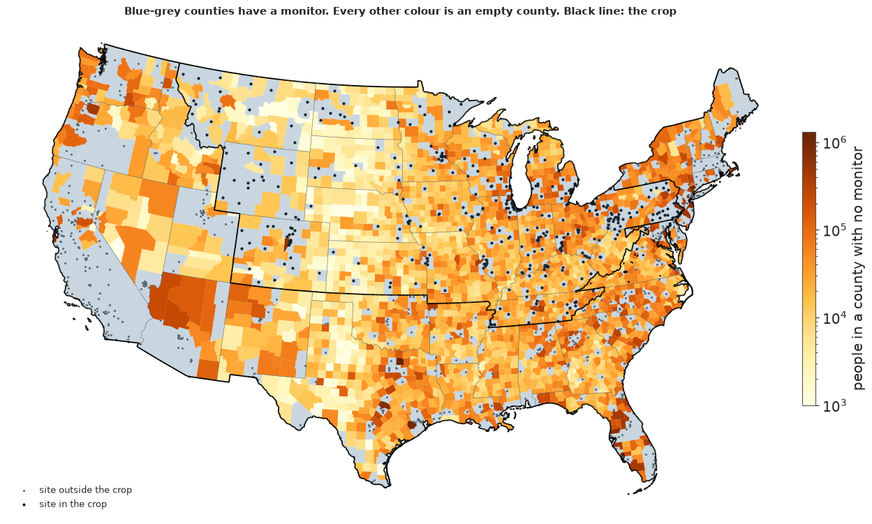
Four in five counties have no monitor, and they hold about 30% of the people, 103 million. Empty does not always mean small: the darkest empty counties have hundreds of thousands of residents.
The crop holds 419 sites and 1,535 counties, 1,242 of them empty. It joins the Midwest and Ohio Valley, where many sites sit near the standard, with the empty, clean Plains and Rockies. New Jersey lies outside it, so a pick in eastern Pennsylvania sees a field cut off at the edge.
Failure 1: two versions of the same instrument
Before any model runs, the daily file holds two versions of the same instruments. EPA's advisory of 26 August 2024 says to drop the original Teledyne T640 series, methods 236 and 238, which corrected series replace. The originals are 20.8% of the 2023 rows and sit under different POC numbers, so nothing marks them as duplicates. A first pass that kept them, or took the maximum over POCs, gave a 2023 mean of 8.54 µg/m³ against 8.22 once clean. Each dot below is one site-series in 2023, on the days both versions report.
pairs = data.load("e89_t640_pairs")
pairs["flips"] = (pairs["original"] >= LINE) & (pairs["corrected"] < LINE)
print(pairs.groupby("pair").agg(sites=("site", "size"), site_days=("days", "sum"),
                                original=("original", "mean"), corrected=("corrected", "mean"),
                                above_only_in_original=("flips", "sum")).round(2).to_string())
print(f"Mean gap {(pairs['original'] - pairs['corrected']).mean():.2f} {UG}; "
      f"{pairs['flips'].sum()} site-series change sides of {LINE}")

low, high = 4.0, 15.0
fig, ax = plt.subplots(figsize=(6.8, 6), layout="constrained")
ax.axvspan(LINE, high, ymin=0, ymax=(LINE - low) / (high - low), color=ABOVE, alpha=0.08, lw=0)
ax.scatter(pairs.loc[~pairs["flips"], "original"], pairs.loc[~pairs["flips"], "corrected"], s=12,
           c=MUTED, lw=0, label="same side either way")
ax.scatter(pairs.loc[pairs["flips"], "original"], pairs.loc[pairs["flips"], "corrected"], s=20, c=ABOVE,
           lw=0, label="above the line only in the superseded data")
ax.plot([low, high], [low, high], color="k", lw=0.8)
ax.axvline(LINE, color="k", lw=0.8, ls=":")
ax.axhline(LINE, color="k", lw=0.8, ls=":")
ax.set(xlim=(low, high), ylim=(low, high), xlabel=f"original T640 series, 2023 mean ({UG})",
       ylabel=f"corrected series, same days ({UG})")
off_chart = ((pairs["original"] > high) | (pairs["original"] < low) | (pairs["corrected"] < low)).sum()
ax.set_title(f"Each dot is one site-series at one of {pairs['site'].nunique()} sites. {off_chart} series below 4 or "
             "above 15 are off the chart", fontsize=11)
ax.legend(loc="upper left");
            sites  site_days  original  corrected  above_only_in_original
pair
236 vs 736    260      55784     10.74       9.57                      47
238 vs 738    133      27166      9.77       8.67                      13
Mean gap 1.14 µg/m³; 60 site-series change sides of 9.05
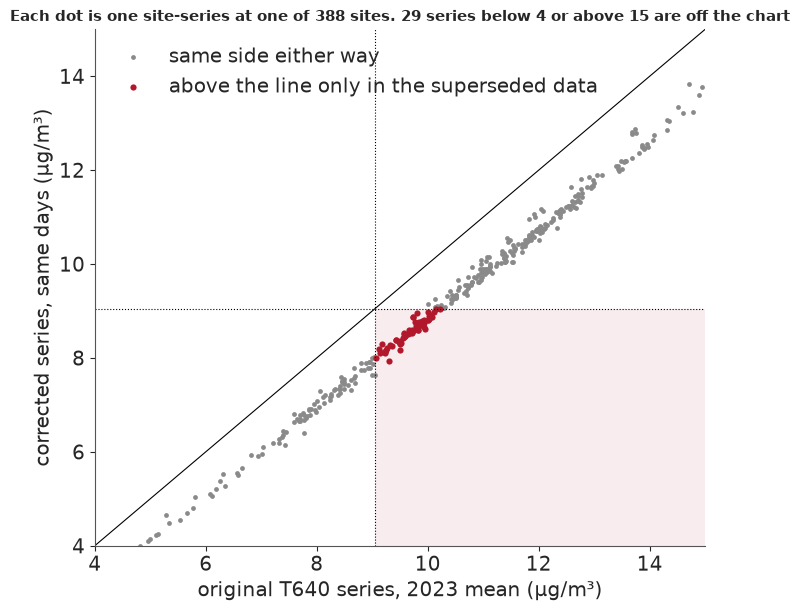
The two versions run side by side at 393 site-series, and the original reads 1.14 µg/m³ high on average. That is the width of the near-line margin: 60 site-series change sides of 9.05, the red dots in the shaded box. A model fitted to the raw file would learn a wrong map of exactly the places this question is about, and nothing in the fit would complain.
EPA's annual summary files cannot fix this, because their 2023 rows say "Multiple Methods Used" and still hold the original data. So every annual value here is rebuilt from the daily files, as the mean over the surviving POCs, never the maximum. The table compares the result with EPA's 2023-2025 design-value workbook.
epa = pd.DataFrame(checks["epa_comparison"]).T[
    ["sites", "median_abs", "p90_abs", "agree_9.05", "sites_dv_8_10", "agree_9.05_dv_8_10"]]
epa.index = ["No concurred events", "All valid sites", "Both FRM and T640 present"]
print(epa.astype(float).round(3).to_string())
                           sites  median_abs  p90_abs  agree_9.05  sites_dv_8_10  agree_9.05_dv_8_10
No concurred events        386.0       0.029    0.153       0.995           91.0               0.978
All valid sites            820.0       0.033    0.222       0.980          282.0               0.943
Both FRM and T640 present  231.0       0.076    0.446       0.957          121.0               0.917
Close: a median gap of 0.03 µg/m³. The column that matters is the last, sites with a design value of 8-10, since far from the line agreement is easy. There 92-98% of sites fall on the same side of 9.05 as EPA's value, worst at sites that run both FRM and T640. These means are close to official design values, but they are not design values.
Smoke stays in
A three-year mean hides its worst days. The ribbon shows the share of US site-days above 35 µg/m³, by day and latitude. Regulators can set aside days that EPA agrees were exceptional events, such as wildfire smoke. We keep them, because our question is about exposure, and smoke is exposure.
ribbon = data.load("e89_ribbon")
bands = [str(b) for b in range(25)]
edges = np.linspace(24, 50, 26)
fig, axes = plt.subplots(3, 1, figsize=(11, 5.6), sharex=True, layout="constrained")
for ax, (year, part) in zip(axes, ribbon.groupby("year")):
    grid = part.set_index("day")[bands].reindex(range(1, 367)).to_numpy(float).T
    mesh = ax.pcolormesh(np.arange(0.5, 367), edges, np.ma.masked_less_equal(np.nan_to_num(grid), 0),
                         cmap="YlOrRd", norm=Normalize(0, 0.5), rasterized=True)
    ax.set(ylabel=f"{year}\nlatitude", yticks=[30, 40, 50])
ax.set_xticks([1, 91, 182, 274, 335], ["Jan", "Apr", "Jul", "Oct", "Dec"])
axes[0].set_title("The worst days arrive in sheets: share of site-days above 35 " + UG, fontsize=11)
fig.colorbar(mesh, ax=axes, shrink=0.7, label="share of site-days");
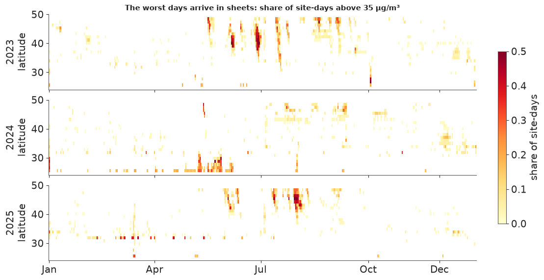
Most of the year is blank; then a sheet crosses many degrees of latitude in days. 2023 has the most summer sheets across 40-50° N, 2024 fewer, and 2025 a dense run from June to August. A site that missed a year missed its sheets, which is why the model carries a term for the years a site reported.
A sparse schedule is measurement error
Many sites sample one day in three or one in six. We thinned near-daily sites to each schedule and compared the thinned annual mean with the full-year one. The data script predicts that error from a variance formula, which enters the model as each site's known noise, $v_s$. The table compares the realised error with the formula's, in µg/m³.
schedule = pd.DataFrame({(year, name): {"realised rms": row[f"1_in_{k}"]["rms"],
                                        "formula rms": row[f"1_in_{k}"]["formula_rms"]}
                         for year, row in checks["schedule_error"].items()
                         for k, name in ((3, "1-in-3"), (6, "1-in-6"), (12, "1-in-12"))})
print(schedule.round(2).to_string())
               2023                  2024                  2025
             1-in-3 1-in-6 1-in-12 1-in-3 1-in-6 1-in-12 1-in-3 1-in-6 1-in-12
realised rms   0.31   0.65    1.12   0.26   0.47    0.71   0.26   0.50    0.84
formula rms    0.56   0.89    1.32   0.36   0.57    0.84   0.41   0.65    0.97
The formula's error runs above the realised error at every schedule in all three years, so it errs on the side of caution. At the sparsest, 1-in-12, the margin is thin: a site's error divided by its own formula sd has an rms of 0.99-1.16 across the years. This bounds the error of a thinned schedule. It does not show that a model of the daily values would give the same answer, and that model was not run.
2 · The model, on a map
One row per site. Let $y_s$ be the log of the site's window mean and $v_s$ its known sampling variance:
$$y_s \sim \text{Normal}\big(\alpha + \beta_d\,\text{density}_s + w_s^\top\beta_m + a_s^\top\delta + f(s),\; \tau_{\text{scale}(s)}^2 + v_s\big), \qquad f \sim \text{GP}\big(0,\ \eta^2\,\text{Matern}_{3/2}(\ell)\big).$$
In words: pollution is a smooth field over the map, plus a term for how crowded the county is, plus corrections for which instruments and which years a site happens to have.
Density, log people per km², is the one covariate that exists at empty counties as well as at monitors. The method shares $w_s$ put every site on an FRM footing, because continuous T640 and BAM instruments do not read exactly like the filter-based reference method. The year mix $a_s$ is a sum-to-zero offset, because a site that missed 2023 missed the smoke. Each measurement scale gets its own nugget $\tau$, the scatter of a site around the smooth field, so a microscale site is not taken for a neighbourhood average. The scale changes a site's spread only, not its mean, and section 3 shows where that falls short.
The field is integrated out: given the hyperparameters the site values are jointly Gaussian, so
PyMC sees one 419 × 419 MvNormal with 15 free parameters, and NUTS never explores 419 latent
values. The field at the county centres comes back afterwards, exactly, one draw at a time.
The priors are LogNormal on the three scales, with the lengthscale centred on 400 km. We draw whole
prior fields at the county centres in NumPy, since pm.sample_prior_predictive gives only sites.
def design(frame, scale=None):
    """What the model needs per site. Density is standardised here unless a scale is given."""
    density = frame["log_density"].to_numpy(float)
    centre, spread = scale or (density.mean(), density.std())
    has = frame[[f"has_{y}" for y in YEARS]].to_numpy(float)
    xy = frame[["x_km", "y_km"]].to_numpy(float)
    return {"site": frame["site"].to_numpy(str), "y": frame["log_mean"].to_numpy(float),
            "v": frame["var_log"].to_numpy(float), "density": (density - centre) / spread,
            "density_scale": (centre, spread),
            "methods": frame[[f"share_{m}" for m in METHODS]].to_numpy(float),
            "years": has / has.sum(axis=1, keepdims=True), "xy": xy, "days": frame["days"].to_numpy(),
            "scale": frame["scale"].map(SCALES.index).to_numpy(int), "distance": distance(xy, xy)}


def distance(a, b):
    return np.sqrt(((a[:, None] - b[None]) ** 2).sum(axis=-1))


def matern32(gap, ell):
    r = np.sqrt(3.0) * gap / ell
    return (1 + r) * np.exp(-r)


def m1(d, method_prior=(0.0, 0.2)):
    """The field integrated out: a marginal GP with 15 free parameters."""
    coords = {"method": METHODS, "year": YEARS, "scale": SCALES, "site": d["site"]}
    with pm.Model(coords=coords) as model:
        alpha = pm.Normal("alpha", 2.0, 0.5)
        beta_density = pm.Normal("beta_density", 0.0, 0.2)
        beta_method = pm.Normal("beta_method", *method_prior, dims="method")
        delta = pm.ZeroSumNormal("delta", sigma=0.1, dims="year")
        mu = (alpha + beta_density * d["density"] + pm.math.dot(d["methods"], beta_method)
              + pm.math.dot(d["years"], delta))
        eta = pm.LogNormal("eta", *PRIOR_ETA)
        ell = pm.LogNormal("ell", *PRIOR_ELL)
        tau = pm.LogNormal("tau", *PRIOR_TAU, dims="scale")
        r = np.sqrt(3.0) * pt.constant(d["distance"]) / ell
        cov = eta ** 2 * (1 + r) * pt.exp(-r) + pt.diag(tau[d["scale"]] ** 2 + d["v"])
        pm.MvNormal("y", mu=mu, cov=cov, observed=d["y"], dims="site")
    return model


d = design(crop_sites)
xy_county = table[["x_km", "y_km"]].to_numpy(float)
gap_county = distance(xy_county, xy_county)
density_county = (table["log_density"].to_numpy(float) - d["density_scale"][0]) / d["density_scale"][1]

with stage("prior check"):
    prior_rng = np.random.default_rng(RANDOM_SEED)
    rows = []
    for _ in range(200):
        eta, ell = prior_rng.lognormal(*PRIOR_ETA), prior_rng.lognormal(*PRIOR_ELL)
        tau = prior_rng.lognormal(*PRIOR_TAU, size=len(SCALES))
        mean = (prior_rng.normal(2.0, 0.5) + prior_rng.normal(0, 0.2) * d["density"]
                + d["methods"] @ prior_rng.normal(0, 0.2, size=3))
        cov = eta ** 2 * matern32(d["distance"], ell) + np.diag(tau[d["scale"]] ** 2 + d["v"])
        rows.append(prior_rng.multivariate_normal(mean, cov, method="cholesky"))
    prior_y = np.array(rows)
    print(pd.DataFrame({"prior 5%": [np.quantile(prior_y.std(axis=1), 0.05),
                                     np.quantile(np.exp(prior_y).mean(axis=1), 0.05)],
                        "prior 95%": [np.quantile(prior_y.std(axis=1), 0.95),
                                      np.quantile(np.exp(prior_y).mean(axis=1), 0.95)],
                        "observed": [d["y"].std(), np.exp(d["y"]).mean()]},
                       index=["sd of log site means", f"crop mean ({UG})"]).round(2).to_string())

    fig, axes = plt.subplots(2, 3, figsize=(12.5, 4.5), layout="constrained")
    for ax, q in zip(axes.flat, (0.05, 0.25, 0.45, 0.6, 0.8, 0.95)):  # ell across its prior, short to long
        ell = np.exp(PRIOR_ELL[0] + PRIOR_ELL[1] * ndtri(q))
        eta = prior_rng.lognormal(*PRIOR_ETA)
        lower = linalg.cholesky(eta ** 2 * matern32(gap_county, ell) + 1e-6 * np.eye(len(table)), lower=True)
        world = (prior_rng.normal(2.0, 0.5) + prior_rng.normal(0, 0.2) * density_county
                 + lower @ prior_rng.normal(size=len(table)))
        shapes = paint(ax, np.exp(world), "RdBu_r", TwoSlopeNorm(LINE, 3.0, 25.0))
        ax.set_title(f"ell = {ell:.0f} km, eta = {eta:.2f}", fontsize=9)
    fig.colorbar(shapes, ax=axes, shrink=0.7, label=f"annual PM2.5 ({UG})")
    fig.suptitle("Before any data: six worlds the priors allow, with ell stepped across its prior. "
                 "White is 9.05", fontsize=11)
    del lower, world, prior_y
    gc.collect();
                      prior 5%  prior 95%  observed
sd of log site means      0.17       0.56      0.28
crop mean (µg/m³)         3.03      19.45      7.64
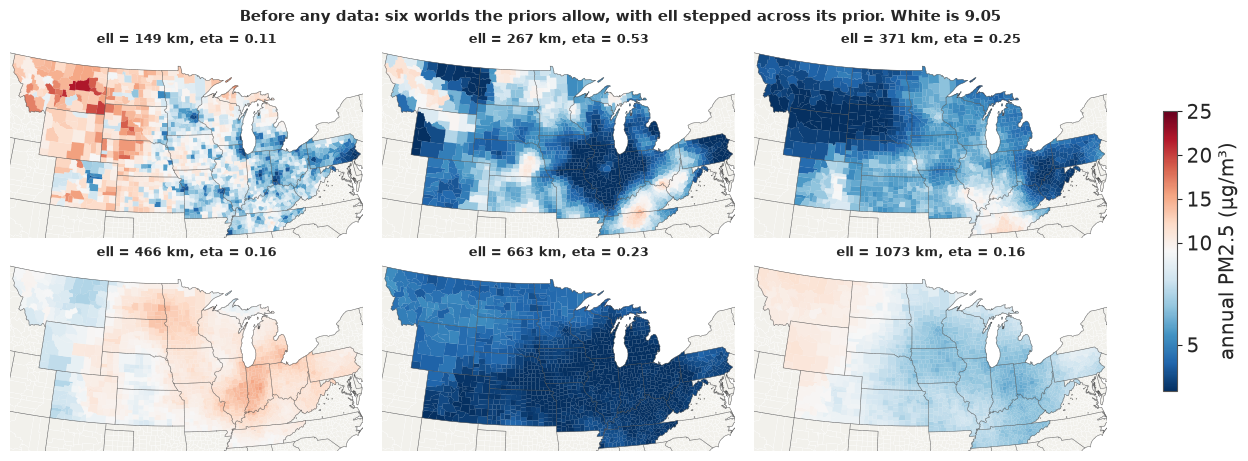
The priors are wide but not silly. The observed spread of log site means (0.28) and crop mean (7.6
µg/m³) sit well inside the prior's 90% ranges, 0.17-0.56 and 3-19 µg/m³. The six worlds run from
patchy at a short ell to one regional tone at a long one.
Now the fit: nutpie through pm.sample, four chains, 400 tuning steps and 500 draws each, one
BLAS thread per chain. Later sections need only 200 evenly spaced draws, and this model mixes well.
NAMES = ("alpha", "beta_density", "beta_method", "delta", "eta", "ell", "tau")


def fit_m1(design_table, seed, **options):
    with m1(design_table, **options):
        return pm.sample(draws=500, tune=400, chains=4, cores=CHAINS_AT_ONCE, random_seed=seed,
                         progressbar=False, compute_convergence_checks=False)


def draws_of(idata):
    """Parameters as plain arrays, (chain, draw, ...): all that the rest of the notebook needs."""
    return {name: idata.posterior[name].to_numpy() for name in NAMES}


with stage("fit M1"):
    idata = fit_m1(d, RANDOM_SEED)
summary = az.summary(idata, var_names=list(NAMES), ci_prob=0.9, ci_kind="eti", round_to=3)
print(summary.to_string())
print(f"max r_hat {summary['r_hat'].astype(float).max():.3f}; "
      f"min bulk ESS {summary['ess_bulk'].astype(float).min():.0f}; "
      f"min tail ESS {summary['ess_tail'].astype(float).min():.0f}; "
      f"divergences {int(idata.sample_stats['diverging'].sum())}; "
      f"tuning steps {idata.posterior.attrs.get('tuning_steps', 'not recorded')}; "
      f"mean leapfrogs {idata.sample_stats['n_steps'].mean().item():.1f}")
fit = draws_of(idata)
                        mean      sd  eti90_lb  eti90_ub  ess_bulk  ess_tail  r_hat  mcse_mean  mcse_sd
alpha                  1.961   0.080     1.830     2.089  2223.855  1431.681  1.004      0.002    0.002
beta_density           0.087   0.013     0.066     0.108  3500.384  1621.625  1.005      0.000    0.000
beta_method[T640]      0.033   0.029    -0.015     0.080  1894.970  1652.656  1.002      0.001    0.001
beta_method[BAM]      -0.111   0.035    -0.168    -0.055  1982.255  1572.491  1.001      0.001    0.001
beta_method[other]     0.007   0.043    -0.066     0.077  2177.948  1566.117  1.003      0.001    0.001
delta[2023]            0.112   0.029     0.064     0.159  3384.639  1910.844  1.001      0.001    0.001
delta[2024]           -0.067   0.039    -0.131    -0.002  3825.586  1740.197  1.000      0.001    0.001
delta[2025]           -0.045   0.029    -0.095     0.005  4017.460  1662.501  0.999      0.000    0.001
eta                    0.243   0.040     0.190     0.320  1826.178  1257.775  1.001      0.001    0.001
ell                  310.422  81.422   208.613   471.808  1265.365  1352.819  1.001      2.372    2.132
tau[NEIGHBORHOOD]      0.121   0.009     0.107     0.136  2254.087  1770.543  1.002      0.000    0.000
tau[URBAN SCALE]       0.109   0.013     0.089     0.130  3809.262  1748.172  1.003      0.000    0.000
tau[REGIONAL SCALE]    0.114   0.019     0.084     0.146  2305.695  1707.246  1.000      0.000    0.000
tau[MIDDLE SCALE]      0.103   0.018     0.077     0.133  3117.619  1329.164  1.002      0.000    0.000
tau[MICROSCALE]        0.139   0.030     0.097     0.195  3385.490  1499.135  1.004      0.001    0.001
tau[unknown]           0.166   0.041     0.112     0.237  3583.379  1559.635  1.002      0.001    0.001
max r_hat 1.005; min bulk ESS 1265; min tail ESS 1258; divergences 0; tuning steps 400; mean leapfrogs 6.9
A clean fit in under 2.5 minutes on 2 cores: no divergences, r_hat at most 1.005, every ESS above 1,200. On the log scale, coefficients read as percentages.
The lengthscale ell is about 310 km (90% interval 210-470), well inside its prior, so the data set
it. Each standard deviation of log density adds about 9% to PM2.5, and 2023 ran about 12% above the
window's average year: the smoke again.
The method term needs care. BAM reads about 10% below FRM, and T640 about 3% above with an interval that spans zero. Instruments compared side by side, at one site on one day, say about -3% and +6%. The model learns this term across sites, and BAM sites tend to be rural, so it can absorb rural air as well as instrument bias. Section 8 refits with the side-by-side pairs as a prior.
The site nugget tau is 10-17%, depending on scale. Remember it: a monitor's reading differs
from the smooth regional field by about that much, and in section 4 that decides what a monitor can
settle about its own county.
ell matters most, because it says how far one monitor can see. Here it is as correlation against
distance, before and after the data.
km = np.linspace(1, 900, 90)
prior_ell = np.random.default_rng(RANDOM_SEED).lognormal(*PRIOR_ELL, size=2000)
post_ell = fit["ell"].ravel()
fig, ax = plt.subplots(figsize=(7.5, 3.6), layout="constrained")
for sample, colour, label in ((prior_ell, MUTED, "prior"), (post_ell, BELOW, "posterior")):
    bands_ = matern32(km[:, None], sample[None])
    low, mid, high = np.quantile(bands_, [0.05, 0.5, 0.95], axis=1)
    ax.fill_between(km, low, high, color=colour, alpha=0.25, lw=0)
    ax.plot(km, mid, color=colour, label=label)
ax.set(xlabel="distance between two places (km)", ylabel="correlation of the field",
       title="How far one monitor can see", ylim=(0, 1), xlim=(0, 900))
ax.legend();
reach = {k: float(np.median(matern32(k, post_ell))) for k in (100, 200, 400)}
print({f"{k} km": round(v, 2) for k, v in reach.items()})
{'100 km': 0.88, '200 km': 0.67, '400 km': 0.32}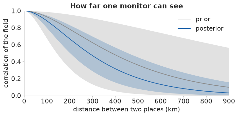
The data pull the prior's wide band in to a narrow one. At the posterior median, places 100 km apart have a correlation of 0.88, at 200 km 0.67 and at 400 km 0.32: a monitor tells us a lot about its neighbours and a little about the next state.
3 · Can the map see what it has not measured?
Every recommendation is about places with no monitor, so we judge the model on places it has not
seen. We use three checks. The first simulates new networks from 200 draws and compares them with
ours. The second holds out one site at a time, and then whole 200 km blocks, which is closer to what
an empty county faces. The third holds out the new sites, first seen in 2023 or later, and
predicts them from the older ones, though the hyperparameters did see them. The hold-outs use the
median hyperparameters and the inverse of the site covariance, which gives every held-out prediction
in closed form (az.loo would see one observation from an MvNormal).
def site_mean(design_table, draw):
    return (draw["alpha"] + draw["beta_density"] * design_table["density"]
            + design_table["methods"] @ draw["beta_method"] + design_table["years"] @ draw["delta"])


def median_draw(chains):
    return {k: np.median(v.reshape(-1, *v.shape[2:]), axis=0) for k, v in chains.items()}


def site_covariance(design_table, draw):
    return (draw["eta"] ** 2 * matern32(design_table["distance"], draw["ell"])
            + np.diag(draw["tau"][design_table["scale"]] ** 2 + design_table["v"]))


def hold_out(precision_matrix, residual, groups):
    """Leave each group out, from the precision matrix: errors and sds of the held-out sites."""
    error, sd = np.empty_like(residual), np.empty_like(residual)
    scaled = precision_matrix @ residual
    for group in groups:
        cov = np.linalg.inv(precision_matrix[np.ix_(group, group)])
        error[group] = cov @ scaled[group]
        sd[group] = np.sqrt(np.diag(cov))
    return error, sd


def scorecard(error, sd):
    return {"sites": error.size, "bias": error.mean(), "se of bias": error.std() / np.sqrt(error.size),
            "rmse": np.sqrt((error ** 2).mean()), "mean predictive sd": sd.mean(),
            "90% coverage": (np.abs(error / sd) < 1.645).mean()}


with stage("checks"):
    best = median_draw(fit)
    residual = d["y"] - site_mean(d, best)
    precision_sites = np.linalg.inv(site_covariance(d, best))
    n_sites = len(residual)

    # replicated networks, one per posterior draw
    stacked = {k: v.reshape(-1, *v.shape[2:]) for k, v in fit.items()}
    check_rng = np.random.default_rng(RANDOM_SEED)
    stats = []
    for i in check_rng.choice(stacked["ell"].size, 200, replace=False):
        draw = {k: v[i] for k, v in stacked.items()}
        replica = check_rng.multivariate_normal(site_mean(d, draw), site_covariance(d, draw),
                                                method="cholesky")
        stats.append((replica.std(), ((replica > np.log(8)) & (replica < np.log(10))).mean(), replica.max()))
    stats = np.array(stats)
    observed = (d["y"].std(), ((d["y"] > np.log(8)) & (d["y"] < np.log(10))).mean(), d["y"].max())
    print(pd.DataFrame(np.c_[np.quantile(stats, [0.05, 0.95], axis=0).T, observed],
                       columns=["replicated 5%", "replicated 95%", "observed"],
                       index=["sd of log means", "share of sites in 8-10", "largest log mean"]).round(3).to_string())

    # one site, 200 km blocks, and the new sites
    cells = pd.factorize(pd.Series(zip((d["xy"][:, 0] // 200).astype(int), (d["xy"][:, 1] // 200).astype(int))))[0]
    is_new = crop_sites["first_year"].to_numpy() >= 2023
    old_near = distance(d["xy"][is_new], d["xy"][~is_new]).min(axis=1)
    new_groups = [np.flatnonzero(is_new)]
    new_error, new_sd = hold_out(precision_sites, residual, new_groups)
    one_error, one_sd = hold_out(precision_sites, residual, [[i] for i in range(n_sites)])
    block_error, block_sd = hold_out(precision_sites, residual, [np.flatnonzero(cells == c) for c in np.unique(cells)])
    far = old_near > 25
    print(pd.DataFrame({"one site": scorecard(one_error, one_sd),
                        "200 km block": scorecard(block_error, block_sd),
                        "new sites": scorecard(new_error[is_new], new_sd[is_new]),
                        "new sites over 25 km": scorecard(new_error[is_new][far], new_sd[is_new][far])}
                       ).T.round(3).to_string())
    near_line = (np.exp(d["y"][is_new]) > 8) & (np.exp(d["y"][is_new]) < 10)
    print(f"New sites over 25 km with a window mean of 8-10: {(far & near_line).sum()}")
    by_scale = pd.DataFrame({"scale": crop_sites["scale"], "error": one_error}).groupby("scale")["error"]
    print(pd.DataFrame({"sites": by_scale.size(), "mean held-out error": by_scale.mean(),
                        "se": by_scale.std() / np.sqrt(by_scale.size())}).round(3).to_string())

    order = np.argsort(old_near)
    fig, ax = plt.subplots(figsize=(7.5, 5.6), layout="constrained")
    centre = (d["y"] - new_error)[is_new][order]
    half = 1.645 * new_sd[is_new][order]
    seen = d["y"][is_new][order]
    missed = np.abs(seen - centre) > half
    rows = np.arange(is_new.sum())
    ax.hlines(rows, np.exp(centre - half), np.exp(centre + half), color=MUTED, lw=2)
    ax.scatter(np.exp(seen)[~missed], rows[~missed], s=22, c="k", zorder=3, label="observed, inside 90%")
    ax.scatter(np.exp(seen)[missed], rows[missed], s=44, c=ABOVE, marker="X", zorder=3, label="observed, outside 90%")
    ax.axvline(LINE, color="k", lw=0.8, ls=":")
    ax.set_yticks(rows[::4], [f"{km_:.0f} km" for km_ in old_near[order][::4]])
    ax.set(xscale="log", xlabel=f"window mean ({UG})", ylabel="distance to the nearest older site",
           title="New sites, predicted from older ones")
    ax.set_xticks([3, 5, 7, 9, 12], ["3", "5", "7", "9", "12"])
    ax.xaxis.set_minor_formatter(NullFormatter())
    ax.legend(loc="upper center", bbox_to_anchor=(0.5, -0.12), ncol=2, frameon=False);
                        replicated 5%  replicated 95%  observed
sd of log means                 0.214           0.355     0.276
share of sites in 8-10          0.095           0.325     0.422
largest log mean                2.444           3.020     2.467
                      sites   bias  se of bias   rmse  mean predictive sd  90% coverage
one site              419.0 -0.001       0.007  0.142               0.135         0.909
200 km block          419.0  0.011       0.008  0.156               0.151         0.919
new sites              34.0 -0.027       0.027  0.162               0.147         0.882
new sites over 25 km   18.0 -0.096       0.039  0.192               0.163         0.889
New sites over 25 km with a window mean of 8-10: 3
                sites  mean held-out error     se
scale
MICROSCALE         16                0.026  0.038
MIDDLE SCALE       23                0.059  0.019
NEIGHBORHOOD      243               -0.005  0.009
REGIONAL SCALE     55                0.005  0.020
URBAN SCALE        71               -0.023  0.016
unknown            11                0.039  0.053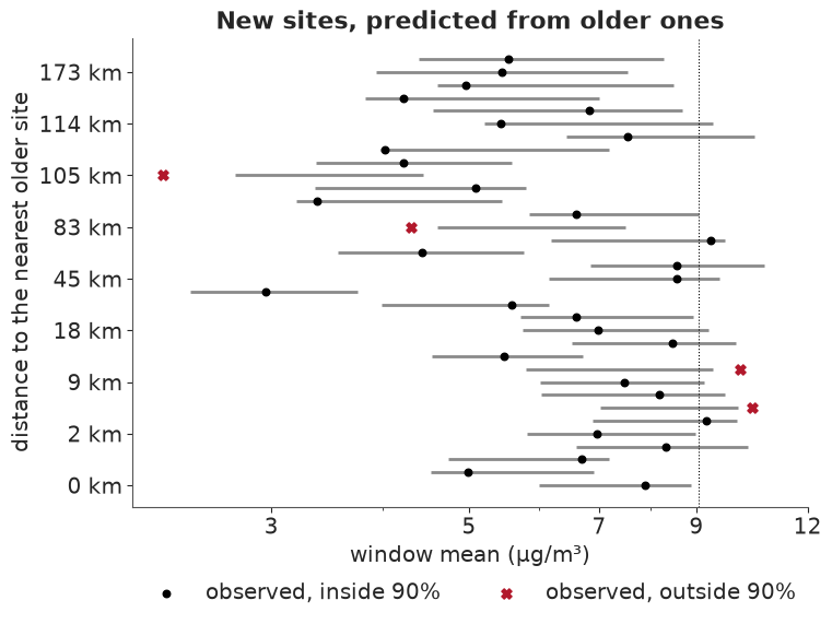
One check fails, and we leave it open. Replicated networks match the spread and the largest value, but 42% of real sites sit between 8 and 10 µg/m³, against 10-33% of replicated ones. Perhaps that is where monitors get placed, perhaps the log-normal shape is wrong; either way, do not over-read fine detail near the line.
Held-out sites behave. Leaving out one site or a whole 200 km block, the error is about 15% and
the 90% intervals cover 91-92%. Block error is only a little larger, as it should be with ell near
310 km.
The new sites are a warning. Overall the model predicts the 34 new sites with almost no bias. But the 18 that lie more than 25 km from any older site read about 9% below prediction (se 4%), and the dots lean left at the top of the figure. That is what a preferentially sited network would produce (Diggle, Menezes & Su 2010): if monitors sit where the air is worse, a model fitted to them reads high in the gaps. So would rural sites near cities. Only 3 of the 18 read near the line, so this cannot check wrong-call rates; the map may run high in empty places.
Middle-scale sites read high, about 6% above prediction (se 2%, 23 sites), while the other scales are within noise. They stand near sources, and the model gives scale no mean term, so they may pull up the field in near-line cities.
4 · Which calls are close?
For each posterior draw, the field at the 1,535 county centres is exactly Gaussian given the sites. We take 200 draws evenly spaced through the chains, so a county's probability of being above the line is a mixture over draws, not a plug-in at the median.
The county covariance over 200 draws would take 1.9 GB, too much for a 3 GB budget. It has a simple form, though: $S = K_{cc} - H^\top H$, the prior covariance less what the 419 sites explain, where $H = L^{-1} K_{sc}$ is 419 × 1,535 and $L$ is the Cholesky factor of the site covariance. The prior part is a formula, so we store only $H$, about 0.5 GB, and build a row of $S$ when we need one. The cell then sets the model's calls against the monitors' own readings and tries three ideas of what a county's truth is.
def thin(chains, count, shift=0):
    """`count` draws evenly spaced through the chains; `shift` moves to a disjoint set."""
    total = chains["ell"].shape[0] * chains["ell"].shape[1]
    take = (np.linspace(0, total - 1, count).round().astype(int) + shift) % total
    return {k: v.reshape(total, *v.shape[2:])[take] for k, v in chains.items()}


def conditional(design_table, draw):
    """Exact mean of the latent field at the county centres, and H, for one draw."""
    lower = linalg.cholesky(site_covariance(design_table, draw), lower=True, check_finite=False)
    cross = draw["eta"] ** 2 * matern32(distance(xy_county, design_table["xy"]), draw["ell"])
    half = linalg.solve_triangular(lower, cross.T, lower=True, check_finite=False)
    residuals = linalg.solve_triangular(lower, design_table["y"] - site_mean(design_table, draw),
                                        lower=True, check_finite=False)
    density = (table["log_density"].to_numpy(float) - design_table["density_scale"][0]) / design_table["density_scale"][1]
    return draw["alpha"] + draw["beta_density"] * density + half.T @ residuals, half  # FRM, whole window


def make_field(design_table, chains, count=200, shift=0):
    """County means, H, and the noise of a new monitor, for `count` draws, as float32."""
    draws = thin(chains, count, shift)
    means = np.empty((count, len(table)), np.float32)
    half = np.empty((count, len(design_table["y"]), len(table)), np.float32)

    def fill(i):
        means[i], half[i] = conditional(design_table, {k: v[i] for k, v in draws.items()})

    with ThreadPoolExecutor(WORKERS) as pool:
        list(pool.map(fill, range(count)))
    noise = draws["tau"][:, SCALES.index("NEIGHBORHOOD")] ** 2 + np.median(design_table["v"][design_table["days"] >= 900])
    return {"means": means, "half": half, "noise": noise, "eta2": np.float32(draws["eta"] ** 2),
            "ells": np.float32(draws["ell"]), "ell": float(np.median(chains["ell"]))}


def covariance_rows(field_, rows_, keep=slice(None)):
    """Rows of S against every county: (draws, len(rows_), counties)."""
    eta2, ells = field_["eta2"][keep][:, None, None], field_["ells"][keep][:, None, None]
    half = field_["half"][keep]
    return eta2 * matern32(gap32[rows_], ells) - half[:, :, rows_].transpose(0, 2, 1) @ half


del idata
gc.collect()
with stage("county conditionals"):
    field = make_field(d, fit)
gap32 = np.float32(gap_county)
variance = field["eta2"][:, None] - (field["half"] ** 2).sum(axis=1)
p_now = ndtr((field["means"] - np.log(LINE)) / np.sqrt(variance)).mean(axis=0)
risk = population * np.minimum(p_now, 1 - p_now)
mean_log = field["means"].mean(axis=0)
sd_log = np.sqrt(variance.mean(axis=0) + field["means"].var(axis=0))
sd_ug = np.exp(mean_log) * sd_log
undecided = (p_now > 0.01) & (p_now < 0.99)
print(f"Expected wrong calls now: {risk.sum() / 1e6:.2f} million people of {population.sum() / 1e6:.1f} million "
      f"(modelled, not observed)")
print(f"Undecided counties (p between 0.01 and 0.99): {undecided.sum()} of {len(table)} ({undecided.mean():.0%})")
print(f"Counties called above 9.0: {(p_now > 0.5).sum()}, holding {population[p_now > 0.5].sum() / 1e6:.1f} million people")
monitored = table["monitored"].to_numpy()
print(f"Share of those wrong-call people in counties that already have a site: {risk[monitored].sum() / risk.sum():.0%}")

readings = pd.DataFrame({"fips": crop_sites["fips"], "reading": np.exp(d["y"]),
                         "settled": ndtr((d["y"] - np.log(LINE)) / np.sqrt(np.maximum(d["v"], 1e-8)))})
readings = readings.groupby("fips").agg(top=("reading", "max"), low=("reading", "min"), settled=("settled", "max"))
readings = table[["fips"]].join(readings, on="fips")
top_site, low_site = readings["top"].to_numpy(), readings["low"].to_numpy()
p_settled = np.where(monitored, readings["settled"].to_numpy(), p_now)
nugget_real = field["noise"][:, None] - np.median(d["v"][d["days"] >= 900])  # tau^2 of a neighbourhood site
p_local = ndtr((field["means"] - np.log(LINE)) / np.sqrt(variance + nugget_real)).mean(axis=0)
called = p_now > 0.5
print(f"Sites against calls: {(top_site >= LINE).sum()} counties have a site at or above {LINE}, and the model calls "
      f"{(called & (top_site >= LINE)).sum()} of them above; {(low_site >= LINE).sum()} have every site above it, and "
      f"{(called & (low_site >= LINE)).sum()} of those are called above")
conventions = pd.DataFrame({
    "people at risk (M)": [(population * np.minimum(p, 1 - p)).sum() / 1e6 for p in (p_settled, p_now, p_local)],
    "of which monitored (M)": [(population * np.minimum(p, 1 - p))[monitored].sum() / 1e6 for p in (p_settled, p_now, p_local)],
    "undecided counties": [((p > 0.01) & (p < 0.99)).sum() for p in (p_settled, p_now, p_local)]},
    index=["a site settles its county (sampling noise only)", "this notebook: truth is the smooth field",
           "the nugget is real air at the county centre"])
print(conventions.round(2).to_string())
worst = np.argsort(-risk)[:8]
print(pd.DataFrame({"people": population[worst].round(), "P(above)": p_now[worst].round(2),
                    "monitored": table["monitored"].to_numpy()[worst],
                    "people at risk of a wrong call": risk[worst].round()},
                   index=short_name[worst]).to_string())
allegheny = int(np.flatnonzero(short_name == "Allegheny PA")[0])
print(f"Allegheny PA: P(above) {p_now[allegheny]:.3f}, top site {top_site[allegheny]:.2f} {UG}, "
      f"{population[allegheny] / 1e6:.2f} million people")

fig, axes = plt.subplots(2, 1, figsize=(12.5, 11), layout="constrained")
shapes = paint(axes[0], p_now, CLOSE_CALL, Normalize(0, 1))
axes[0].scatter(crop_sites["x_km"], crop_sites["y_km"], s=4, c="#d95f02", lw=0)
axes[0].set_title("The call: chance that a county's air is above 9.0. The darkest counties are the closest "
                  "calls. Orange dots are monitors", loc="left", fontsize=11)
fig.colorbar(shapes, ax=axes[0], shrink=0.6, label="P(above 9.0)", pad=0.01)
paint(axes[1], np.where(undecided, 0.5, np.nan), "Greys", Normalize(0, 1))
for mask, colour, label in ((monitored, BELOW, "county with a monitor"), (~monitored, PICK, "empty county")):
    show = mask & (risk > 2e3)
    axes[1].scatter(xy_county[show, 0], xy_county[show, 1], s=risk[show] / 1.5e3, facecolor=colour, alpha=0.65,
                    edgecolor="w", lw=0.4, label=label)
for rank_, i in enumerate(np.argsort(-risk)[:6]):
    axes[1].annotate(short_name[i], xy_county[i], xytext=(0, 12 if rank_ % 2 else -12), textcoords="offset points",
                     fontsize=8, ha="center", va="center", path_effects=[pe.withStroke(linewidth=2.2, foreground="w")])
for size in (1e5, 5e5, 1e6):
    axes[1].scatter([], [], s=size / 1.5e3, facecolor=MUTED, alpha=0.65, edgecolor="w", lw=0.4,
                    label=f"{size / 1e6:g} million at risk")
axes[1].legend(loc="lower left", frameon=True, fontsize=9)
axes[1].set_title("The stakes: people in a county times its chance of a wrong call. "
                  "Grey counties are undecided", loc="left", fontsize=11);
Expected wrong calls now: 10.43 million people of 103.9 million (modelled, not observed)
Undecided counties (p between 0.01 and 0.99): 452 of 1535 (29%)
Counties called above 9.0: 9, holding 10.9 million people
Share of those wrong-call people in counties that already have a site: 89%
Sites against calls: 32 counties have a site at or above 9.05, and the model calls 7 of them above; 12 have every site above it, and 3 of those are called above
                                                 people at risk (M)  of which monitored (M)  undecided counties
a site settles its county (sampling noise only)                1.37                    0.23                 347
this notebook: truth is the smooth field                      10.43                    9.28                 452
the nugget is real air at the county centre                   22.88                   17.96                1272
                    people  P(above)  monitored  people at risk of a wrong call
Cook IL          5182620.0      0.74       True                       1341172.0
Franklin OH      1356300.0      0.52       True                        656042.0
Philadelphia PA  1573920.0      0.37       True                        582519.0
Wayne MI         1771060.0      0.70       True                        536716.0
Oakland MI       1296890.0      0.38       True                        495354.0
Kent MI           673002.0      0.51       True                        328703.0
DuPage IL         937142.0      0.33       True                        311057.0
Hamilton OH       837359.0      0.34       True                        284195.0
Allegheny PA: P(above) 0.000, top site 10.25 µg/m³, 1.23 million people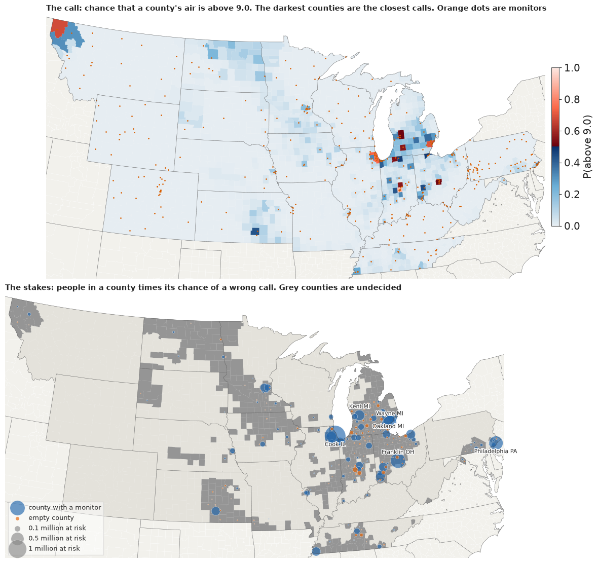
The top map shows how few calls are close. Most of the crop is pale, clearly below the line. Only 9 counties are called above it, but they hold about 11 million people. In all, about 10 million people of 104 million are expected to be on the wrong side, and 452 counties, about 30%, are undecided (a probability of being above between 0.01 and 0.99). These are modelled numbers.
The bottom map holds the surprise. About nine in ten of those people live in counties that already have a monitor, the blue circles; Cook IL alone carries 1.3 million. Franklin OH has four monitors reading 9.05-9.86 and still sits at P = 0.52. Allegheny PA has a site at 10.25 and 1.2 million people, and P is about 0. That is the nugget at work: a site's reading is not the county's smooth field, so a monitor does not settle its county. Of the 32 counties with a site at or above the line, the model calls 7 above; of the 12 where every site is above, it calls 3.
This choice is not the law, under which Franklin's status comes from its monitors, and the table of three conventions shows its size. If a monitored county is settled by its highest site, about 1.4 million people are at risk, and about 1.1 million of them are in empty counties. If the nugget is real air at every county centre, about 23 million are, four in five of them in monitored counties; that is an upper case, since part of the nugget is instrument difference. Our 10 million, between the two, is about the smooth field, not what any one person breathes, and this split decides what the shortlist means.
5 · Uncertainty is not value
The obvious rule is to put monitors where we are most uncertain. The better question is the one from the top: what would we do differently if we knew?
For one candidate county $c$ and one posterior draw, a new reading $y$ has predictive variance $S_{cc} + n$, where $n$ is the noise of a new neighbourhood-scale monitor, and it moves every county's mean by a rank-one Gaussian update. So the value of a monitor at $c$ needs no simulation:
- Take 16 equally likely readings from the predictive distribution of $y$, a mixture over draws.
- For each reading, reweight the draws by how well they predicted it, update each county within each draw, and average over draws to get the county's new $P(\text{above})$.
- The expected loss is the average over readings of $\sum_j \text{people}_j \min(p_j, 1 - p_j)$.
The fall in expected loss is the site's EVSI, in people moved to a right call. To save time we count only counties within $3\ell$ of the candidate that are still undecided.
Two tricks keep this cheap. A score reads only the covariance of a candidate with the undecided counties, so that block is built once. And a pick stores only its low-rank factor, 25 MB for 20 picks, rather than a new covariance, so one field serves every search below.
def reading_nodes(mean, variance_, nodes):
    """Midpoints of `nodes` equal-probability bins of the mixture predictive of the reading."""
    sd = np.sqrt(variance_)
    grid = np.linspace((mean - 6 * sd).min(), (mean + 6 * sd).max(), 256)
    cdf = ndtr((grid[:, None] - mean) / sd).mean(axis=1)
    return np.interp((np.arange(nodes) + 0.5) / nodes, cdf, grid)


def update_weights(y, mean, variance_):
    """Each draw's posterior weight after reading `y` (axes: readings, draws)."""
    log = -0.5 * (y[:, None] - mean) ** 2 / variance_ - 0.5 * np.log(variance_)
    return np.exp(log - logsumexp(log, axis=1, keepdims=True))


def probability_above(y, weights, mu, var, cross, mu_c, q, line):
    """P(above the line) per county after each reading: rank-one update in each draw, then mix."""
    gain = cross / q[:, None]
    shift = (y[:, None] - mu_c)[:, :, None]
    sd = np.sqrt(np.maximum(var - gain * cross, 1e-10))
    return (weights[:, :, None] * ndtr((mu + shift * gain - line) / sd)).sum(axis=1)


def loss(p, weight, objective):
    """Expected loss, calling each county at p = 0.5."""
    if objective == "missed":  # called below, truly above
        return (weight * np.where(p < 0.5, p, 0.0)).sum(axis=-1)
    if objective == "false":   # called above, truly below
        return (weight * np.where(p >= 0.5, 1 - p, 0.0)).sum(axis=-1)
    return (weight * np.minimum(p, 1 - p)).sum(axis=-1)


def open_block(field_, line):
    """Covariance of every candidate with the undecided counties: all a score ever reads."""
    key = f"block_{line}"
    if key not in field_:
        variance_ = field_["eta2"][:, None] - (field_["half"] ** 2).sum(axis=1)
        p = ndtr((field_["means"] - np.float32(np.log(line))) / np.sqrt(variance_)).mean(axis=0)
        where = np.flatnonzero((p > 0.005) & (p < 0.995))  # a wider net than `open`, for subsets of draws
        block = np.empty((len(variance_), len(candidates), where.size), np.float32)
        gaps = gap32[np.ix_(candidates, where)]

        def fill(i):
            half = field_["half"][i]
            block[i] = field_["eta2"][i] * matern32(gaps, field_["ells"][i]) - half[:, candidates].T @ half[:, where]

        with ThreadPoolExecutor(WORKERS) as pool:
            list(pool.map(fill, range(len(block))))
        field_[key] = (block, where)
    return field_[key]


CANDIDATE_ROW = np.full(len(table), -1)
CANDIDATE_ROW[candidates] = np.arange(len(candidates))


class Network:
    """The county field given the monitors picked so far.

    The field is never written to. A pick appends one row of the low-rank factor `u`, and each
    draw's mean stays put, because the reading is unknown. So only the first round is an exact
    value: `joint_value` measures what a whole set is worth.
    """

    def __init__(self, field_, weight=None, line=LINE, objective="wrong", nodes=16, rounds=20,
                 noise_scale=1.0, keep=slice(None), reach=3.0):
        self.field, self.keep = field_, keep
        self.mu = field_["means"][keep]
        self.noise = np.float32(field_["noise"][keep] * noise_scale)
        self.weight = np.float32(population if weight is None else weight)
        self.line, self.objective, self.nodes = np.float32(np.log(line)), objective, nodes
        self.radius = reach * field_["ell"]
        self.u = np.zeros((self.mu.shape[0], rounds, self.mu.shape[1]), np.float32)
        self.k = 0
        block, self.where = open_block(field_, line)
        self.block = block[keep]
        self.var = field_["eta2"][keep][:, None] - (field_["half"][keep] ** 2).sum(axis=1)
        self.refresh()

    def refresh(self):
        self.p = ndtr((self.mu - self.line) / np.sqrt(np.maximum(self.var, 1e-10))).mean(axis=0)
        self.open = (self.p > 0.01) & (self.p < 0.99)

    def column(self, c):
        """Covariance of county `c` with every county, after the picks so far: slower, so for picks."""
        out = covariance_rows(self.field, [c], self.keep)[:, 0]
        if self.k:
            out -= (self.u[:, : self.k, c][:, None] @ self.u[:, : self.k])[:, 0]
        return out

    def value(self, c):
        """Expected fall in the loss from one more monitor at county `c` (EVSI)."""
        slots = np.flatnonzero((gap32[c, self.where] < self.radius) & self.open[self.where])
        if slots.size == 0:
            return 0.0
        local = self.where[slots]
        cross = self.block[:, CANDIDATE_ROW[c]][:, slots]
        if self.k:
            cross = cross - (self.u[:, : self.k, c][:, None] @ self.u[:, : self.k][:, :, local])[:, 0]
        var, mu, mu_c, q = self.var[:, local], self.mu[:, local], self.mu[:, c], self.var[:, c] + self.noise
        y = reading_nodes(mu_c, q, self.nodes)
        p = probability_above(y, update_weights(y, mu_c, q), mu, var, cross, mu_c, q, self.line)
        before = ndtr((mu - self.line) / np.sqrt(var)).mean(axis=0)
        return float(loss(before, self.weight[local], self.objective)
                     - loss(p, self.weight[local], self.objective).mean())

    def score(self, chosen):
        with ThreadPoolExecutor(WORKERS) as pool:
            return np.array(list(pool.map(self.value, chosen)))

    def pick(self, c):
        col = self.column(c)
        self.u[:, self.k] = col / np.sqrt(col[:, c] + self.noise)[:, None]
        self.var = self.var - self.u[:, self.k] ** 2
        self.k += 1
        self.refresh()


net = Network(field)
with stage("first round, every candidate"):
    first_value = np.full(len(table), np.nan)
    first_value[candidates] = net.score(candidates)
ranked = candidates[np.argsort(-first_value[candidates])]
print(f"Best single monitor: {short_name[ranked[0]]}, {first_value[ranked[0]] / 1e3:.0f} thousand people. "
      f"Median candidate: {np.median(first_value[candidates]) / 1e3:.1f} thousand")
print(f"Candidates with EVSI under 1,000 people: {(first_value[candidates] < 1e3).mean():.0%}")
Best single monitor: Delaware OH, 143 thousand people. Median candidate: 4.6 thousand
Candidates with EVSI under 1,000 people: 26%
The best single monitor is in Delaware County, Ohio, just north of Columbus, worth about 140 thousand people moved to a right call. The median candidate is worth under 5 thousand, and a quarter of them under 1,000.
Does the closed form tell the truth?
A formula this convenient needs a test that can fail. For the best candidate we simulate a true field from each draw, draw a noisy reading, make the calls with the closed-form posterior, and count real wrong calls against the simulated truth. As a control we repeat the calls with a reading believed 25 times more precise than it is; that version must fall short.
def brute_force(field_, c, sims=8000, width=150, seed=0, control_factor=25.0):
    """Simulate truth and reading, make the call, and count real wrong calls."""
    check = np.random.default_rng(seed)
    near_c = np.argsort(gap_county[c])[:width]
    mu = field_["means"][:, near_c].astype(float)
    cov = np.stack([eta2 * matern32(gap_county[np.ix_(near_c, near_c)], ell) - half[:, near_c].T @ half[:, near_c]
                    for eta2, ell, half in zip(field_["eta2"], field_["ells"], field_["half"])]).astype(float)
    noise, pop = field_["noise"], population[near_c]
    index = int(np.flatnonzero(near_c == c)[0])
    line = np.log(LINE)
    lower = [linalg.cholesky(s + 1e-7 * np.eye(width), lower=True) for s in cov]
    var = np.einsum("ijj->ij", cov)
    cross, var_c, mu_c = cov[:, index], cov[:, index, index], mu[:, index]
    q = var_c + noise
    before = ndtr((mu - line) / np.sqrt(var)).mean(axis=0) > 0.5
    honest, misled = [], []
    for _ in range(sims // 500):
        which = check.integers(len(mu), size=500)
        truth = np.stack([mu[i] + lower[i] @ check.normal(size=width) for i in which])
        y = truth[:, index] + np.sqrt(noise[which]) * check.normal(size=500)
        above = truth > line
        wrong_before = ((before != above) * pop).sum(axis=1)
        for believed, out in ((q, honest), (var_c + noise / control_factor, misled)):
            p = probability_above(y, update_weights(y, mu_c, believed), mu, var, cross, mu_c, believed, line)
            out.append(wrong_before - (((p > 0.5) != above) * pop).sum(axis=1))
    honest, misled = np.concatenate(honest), np.concatenate(misled)
    y = reading_nodes(mu_c, q, 16)
    after = probability_above(y, update_weights(y, mu_c, q), mu, var, cross, mu_c, q, line)
    closed = float(loss(ndtr((mu - line) / np.sqrt(var)).mean(axis=0), pop, "wrong") - loss(after, pop, "wrong").mean())
    se = honest.std() / np.sqrt(honest.size)
    return {"closed form": closed, "brute force": honest.mean(), "se": se, "z": (closed - honest.mean()) / se,
            "control, reading over-trusted": misled.mean()}


with stage("brute-force check"):
    print({k: round(float(v), 2) for k, v in brute_force(field, int(ranked[0])).items()})
{'closed form': 141311.9, 'brute force': 146164.21, 'se': 10546.47, 'z': -0.46, 'control, reading over-trusted': -50272.75}Closed form 141 thousand, brute force 146 thousand with a standard error of 11 thousand: they agree within half a standard error. The control does worse than no monitor at all, about 50 thousand people worse off, so the test can tell a wrong posterior from a right one. The draws are held fixed, so draw noise is invisible here; section 6 measures it.
Now the centrepiece: what we do not know, against what is worth knowing.
is_candidate = np.zeros(len(table), bool)
is_candidate[candidates] = True
rank_sd = pd.Series(-sd_ug[candidates], index=candidates).rank(method="first").astype(int)
rank_value = pd.Series(-first_value[candidates], index=candidates).rank(method="first").astype(int)
top_sd = rank_sd.sort_values().index[:20].to_numpy()
top_value = rank_value.sort_values().index[:20].to_numpy()
print(f"Top 20 by uncertainty and top 20 by single-monitor value share {len(set(top_sd) & set(top_value))} counties")
print(f"Best EVSI among the 20 most uncertain: {first_value[top_sd].max() / 1e3:.1f} thousand people "
      f"(best overall {first_value[ranked[0]] / 1e3:.0f})")
print(f"Median posterior sd: top 20 by uncertainty {np.median(sd_ug[top_sd]):.2f} {UG}, "
      f"top 20 by value {np.median(sd_ug[top_value]):.2f} {UG}")
print(f"Spearman rank correlation over {len(candidates):,} candidates: {rank_sd.corr(rank_value):.2f}")


def squash(rank):
    """Ranks 1-15 at full size, then a compressed tail down to the last candidate."""
    rank = np.asarray(rank, float)
    return np.where(rank <= 15, rank, 15 + 4 * np.log10(rank / 15))


fig = plt.figure(figsize=(13.5, 9.2), layout="constrained")
grid = fig.add_gridspec(2, 2, width_ratios=[2.5, 1])
ax_sd, ax_value, ax_bump = fig.add_subplot(grid[0, 0]), fig.add_subplot(grid[1, 0]), fig.add_subplot(grid[:, 1])
shapes = paint(ax_sd, np.where(is_candidate, sd_ug, np.nan), "viridis", Normalize(0, np.quantile(sd_ug, 0.995)),
               labels=[(top_sd[0], short_name[top_sd[0]])])
halo = [pe.withStroke(linewidth=1.8, foreground="k")]
ax_sd.scatter(xy_county[top_sd, 0], xy_county[top_sd, 1], s=18, facecolor="none", edgecolor="w", lw=0.8, path_effects=halo)
ax_sd.set_title("What we do not know: posterior sd at empty counties. Rings: the 20 highest", loc="left", fontsize=11)
fig.colorbar(shapes, ax=ax_sd, shrink=0.75, label=f"sd of county mean ({UG})", pad=0.01)
shapes = paint(ax_value, np.where(is_candidate, np.maximum(first_value, 100), np.nan), "magma_r",
               LogNorm(100, np.nanmax(first_value)), labels=[(top_value[0], short_name[top_value[0]])])
ax_value.scatter(xy_county[top_value, 0], xy_county[top_value, 1], s=18, facecolor="none", edgecolor="w", lw=0.8,
                 path_effects=halo)
ax_value.set_title("What is worth knowing: people one monitor moves to a right call. Rings: the 20 highest", loc="left",
                   fontsize=11)
fig.colorbar(shapes, ax=ax_value, shrink=0.75, label="EVSI, people (floor at 100)", pad=0.01)

for ids, colour, align in ((top_sd[:10], PICK, "right"), (top_value[:10], BELOW, "left")):
    for i in ids:
        a, b = squash(rank_sd[i]), squash(rank_value[i])
        ax_bump.plot([0, 1], [a, b], color=colour, lw=1.3, alpha=0.75, marker="o", ms=3)
        x, y_ = (-0.04, a) if align == "right" else (1.04, b)
        ax_bump.text(x, y_, short_name[i], ha=align, va="center", fontsize=8, color=colour)
ticks = [1, 5, 10, 15, 50, 200, len(candidates)]
ax_bump.set_yticks(squash(ticks), [str(t) for t in ticks])
ax_bump.axhline(15.5, color=MUTED, lw=0.8, ls=":")
ax_bump.text(-0.72, 15.65, "ranks below this\nline are compressed", ha="left", va="top", fontsize=7.5, color=MUTED)
ax_bump.set_ylim(squash(len(candidates)) + 0.5, 0.2)
ax_bump.set_xlim(-0.75, 1.75)
ax_bump.set_xticks([0, 1], ["rank by\nuncertainty", "rank by\nvalue"])
ax_bump.grid(False)
foggy_ranks = rank_value[top_sd]
print(f"Value rank of the 20 foggiest: {foggy_ranks.min()}-{foggy_ranks.max()} of {len(candidates):,}, "
      f"median {foggy_ranks.median():.0f}")
ax_bump.set_title("The foggiest counties rank in the lower half by value", fontsize=11);
Top 20 by uncertainty and top 20 by single-monitor value share 0 counties
Best EVSI among the 20 most uncertain: 4.6 thousand people (best overall 143)
Median posterior sd: top 20 by uncertainty 1.05 µg/m³, top 20 by value 0.49 µg/m³
Spearman rank correlation over 1,238 candidates: -0.29
Value rank of the 20 foggiest: 621-1015 of 1,238, median 764
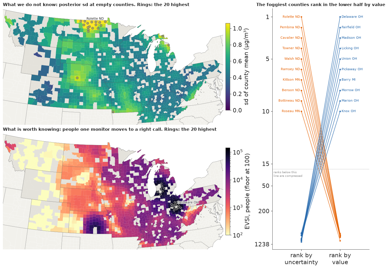
This is the lesson in one picture. The fog lies over the northern Plains; the value sits in a few pockets around Columbus, lower Michigan and Wichita. The 20 most uncertain counties and the 20 most valuable have no county in common, and over all 1,238 candidates the two rankings are negatively correlated (Spearman -0.29). The most uncertain have twice the posterior sd of the most valuable (1.05 against 0.49 µg/m³), and the best of them is worth a thirtieth of Delaware OH. By value they rank between 621st and 1,015th: the lower half, though not the very bottom, since the right panel squeezes every rank below 15.
So a sentence that sounds odd is true: Rolette County, North Dakota, is very uncertain, and it is not worth a monitor. The next figure shows why. For three counties, the horizontal axis is what a new monitor might read. The black curve is how likely each reading is; the colour shows how many people's calls would flip at that reading, and white means none. Value needs the curve and the colour to overlap.
def reading_strip(network, c, grid_ug):
    """People whose call flips, and the predictive density of the reading, at each reading."""
    y = np.log(grid_ug)
    col = network.column(c)
    q = col[:, c] + network.noise
    mu_c = network.mu[:, c]
    local = np.flatnonzero((gap32[c] < network.radius) & network.open)
    p = probability_above(y, update_weights(y, mu_c, q), network.mu[:, local], network.var[:, local],
                          col[:, local], mu_c, q, network.line)
    flipped = ((p > 0.5) != (network.p[local] > 0.5)) * population[local]
    density = (np.exp(-0.5 * (y[:, None] - mu_c) ** 2 / q) / np.sqrt(2 * np.pi * q)).mean(axis=1) / grid_ug
    return flipped.sum(axis=1), density


foggy = int(top_sd[0])
biggest = int(candidates[np.argmax(population[candidates])])
trio = [("The best single site", int(ranked[0])), ("The most uncertain county", foggy),
        ("The most populous empty county", biggest)]
grid_ug = np.linspace(2.5, 16, 271)
fig, axes = plt.subplots(3, 1, figsize=(10.5, 6), sharex=True, layout="constrained")
rows = []
for ax, (title, c) in zip(axes, trio):
    people, density = reading_strip(net, c, grid_ug)
    shown = np.ma.masked_equal(people[None], 0)
    mesh = ax.pcolormesh(grid_ug, [0, 1], np.repeat(shown, 2, axis=0), cmap="magma_r", norm=LogNorm(1e4, 3e7),
                         shading="nearest", rasterized=True)
    ax.plot(grid_ug, 0.92 * density / density.max(), color="k", lw=1.2)
    ax.axvline(LINE, color="k", lw=0.8, ls=":")
    ax.set(yticks=[], ylim=(0, 1))
    ax.set_title(f"{title}: {short_name[c]}. EVSI {first_value[c] / 1e3:.1f} thousand people, "
                 f"sd {sd_ug[c]:.2f} {UG}, {population[c] / 1e3:.0f} thousand residents", loc="left", fontsize=10)
    rows.append({"county": short_name[c], "P(above)": p_now[c], "chance a reading flips any call":
                 float(np.trapezoid(density * (people > 0), grid_ug)), "max people flipped": people.max()})
axes[-1].set_xlabel(f"what the new monitor reads ({UG}); dotted line is the 9.05 standard")
fig.colorbar(mesh, ax=axes, shrink=0.8, label="people whose call flips")
print(pd.DataFrame(rows).round(2).to_string(index=False));
     county  P(above)  chance a reading flips any call  max people flipped
Delaware OH      0.13                             0.74           2682750.0
 Rolette ND      0.20                             0.14            223773.0
    Lake IL      0.04                             0.45           8130150.0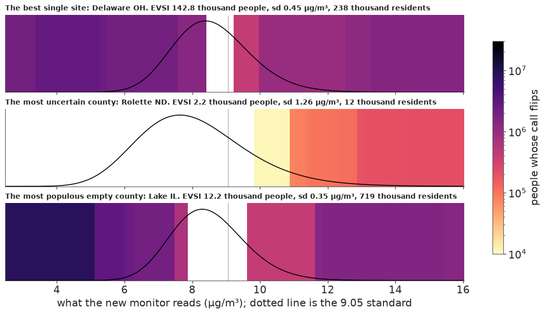
Rolette ND: the curve is wide, which is the fog, but almost all of it lies over white. A call flips only if the reading tops about 10, a 14% chance, and then few people are affected. Delaware OH: the curve is narrower, yet it overlaps colour on both sides, and 74% of readings would flip some call. Lake IL, the most populous empty county, beside Chicago, could flip Chicago's call, and 45% of its readings flip something, yet its EVSI is only about 12 thousand. A flip is necessary but not sufficient: moving a county from 0.51 to 0.49 hardly changes its expected wrong calls.
6 · Choosing twenty sites
One monitor is a formula. Twenty is a search: pick the best, update the field, repeat. Scoring all 1,238 candidates in every round takes minutes, so we use the lazy greedy search (Minoux 1978): it scores everyone once, then rescores only the 50 sites with the best previous scores. That is safe when a site's gain never rises after another pick. Here it is not quite true. In tests on this field, gains rose in three pairs of picks out of four, but only by a median ratio of 1.0002, and the lazy top 20 matched a full greedy search exactly at 100 and 200 draws. To catch a miss anyway, the loop rescores every remaining candidate in its last round.
def lazy_greedy(network, pool=candidates, rounds=20, top=50, recheck=False, start=None):
    """Pick `rounds` sites, rescoring only the best `top` by last score after the first round.

    `start` is a first round already scored, in the order of `pool`.
    """
    pool = np.asarray(pool)
    last = np.full(len(pool), np.inf) if start is None else np.array(start, float)
    free = np.ones(len(pool), bool)
    picks, gains, audit = [], [], None
    for round_ in range(rounds):
        todo = np.flatnonzero(free)
        lazy = todo[np.argsort(-last[todo])[: top]] if round_ > 0 else todo
        full_round = recheck and round_ == rounds - 1
        if round_ > 0 or start is None:
            last[todo if full_round else lazy] = network.score(pool[todo if full_round else lazy])
        best = lazy[np.argmax(last[lazy])]
        if full_round:
            everyone = pd.Series(last[todo], index=pool[todo]).rank(ascending=False)
            audit = {"lazy choice": short_name[pool[best]], "its rank in the full rescore": int(everyone[pool[best]]),
                     "full-rescore choice": short_name[pool[todo[np.argmax(last[todo])]]],
                     "candidates rescored": len(todo)}
        if last[best] <= 0:
            break
        picks.append(int(pool[best]))
        gains.append(float(last[best]))
        free[best] = False
        network.pick(int(pool[best]))
    return {"picks": picks, "gains": gains, "audit": audit, "network": network}


with stage("lazy greedy, 200 draws"):
    main = lazy_greedy(Network(field), recheck=True, start=first_value[candidates])
print("Final-round audit:", main["audit"])
print("Picks in order of the search, not of merit:")
print(", ".join(short_name[main["picks"]]))
print(f"Sum of greedy gains: {sum(main['gains']) / 1e6:.2f} million people")
Final-round audit: {'lazy choice': 'Greene OH', 'its rank in the full rescore': 1, 'full-rescore choice': 'Greene OH', 'candidates rescored': 1219}
Picks in order of the search, not of merit:
Delaware OH, Fairfield OH, Madison OH, Barry MI, Licking OH, Union OH, Pickaway OH, Ionia MI, Van Buren MI, Muskegon MI, Calhoun MI, Morrow OH, Montcalm MI, St. Joseph MI, Fayette OH, Champaign OH, Newaygo MI, Cass MI, Eaton MI, Greene OH
Sum of greedy gains: 1.72 million people
The last-round check passes: the lazy choice, Greene OH, is also the best of all 1,219 remaining candidates, though that checks the last round only. The 20 picks fall into two tight clusters, ten around Columbus and ten in lower Michigan. The printed order is the order of the search, not of merit, because each pick depends on the ones before it and only the first is scored exactly.
Is this list about the air, or about our draws? Split the draws and search each part. A list we could hand over as a ranking would need most picks to survive, say 16 of 20. Here are four disjoint sets of 50 draws, compared in pairs, and two sets of 100.
def overlap(a, b):
    return len(set(a) & set(b))


with stage("split-half runs"):
    quarters = [lazy_greedy(Network(field, keep=slice(i, None, 4)))["picks"] for i in range(4)]
    halves = [lazy_greedy(Network(field, keep=slice(i, None, 2)))["picks"] for i in range(2)]
overlap_50 = [overlap(a, b) for i, a in enumerate(quarters) for b in quarters[i + 1:]]
overlap_100 = overlap(*halves)
print(f"Top-20 overlap, 50 draws against 50:   {overlap_50}")
print(f"Top-20 overlap, 100 draws against 100: {overlap_100}")
Top-20 overlap, 50 draws against 50:   [16, 16, 15, 17, 16, 19]
Top-20 overlap, 100 draws against 100: 17
Failure 2: a ranked list does not survive new draws
The 50-draw pairs share 15 to 19 picks and the two 100-draw lists 17. On other runs of the notebook the pairs went as low as 13, and more draws did not steadily help, so read it as about 17 of 20, sometimes 13. That alone rules out a fixed ranked list: the last places change with the random draws. The picks stay close, though: 90-100% of one half's picks lie within 100 km of a pick from the other half.
How far does a set reach? The maps show the share of each county's uncertainty removed after 5, 10 and 20 picks: how much fog lifts, not which way a county moves. The picks crowd into the gaps between existing sites, and their effect fades within about 200 km.
box = xy_county[main["picks"]]
window = dict(xlim=(box[:, 0].min() - 260, box[:, 0].max() + 260), ylim=(box[:, 1].min() - 260, box[:, 1].max() + 260))
fig, axes = plt.subplots(1, 3, figsize=(13, 4.8), layout="constrained")
for ax, k in zip(axes, (5, 10, 20)):
    after = variance - (main["network"].u[:, : k] ** 2).sum(axis=1)
    shapes = paint(ax, 1 - after.mean(axis=0) / variance.mean(axis=0), "BuPu", Normalize(0, 0.6))
    chosen = main["picks"][: k]
    ax.scatter(crop_sites["x_km"], crop_sites["y_km"], s=7, c="k", lw=0)
    ax.scatter(xy_county[chosen, 0], xy_county[chosen, 1], s=30, c=PICK, edgecolor="w", lw=0.6, zorder=3)
    ax.set(**window)
    ax.set_title(f"After {k} new monitors", loc="left", fontsize=11)
fig.colorbar(shapes, ax=axes, shrink=0.7, label="share of uncertainty removed")
fig.suptitle("Orange: new monitors. Black: existing sites", fontsize=11);
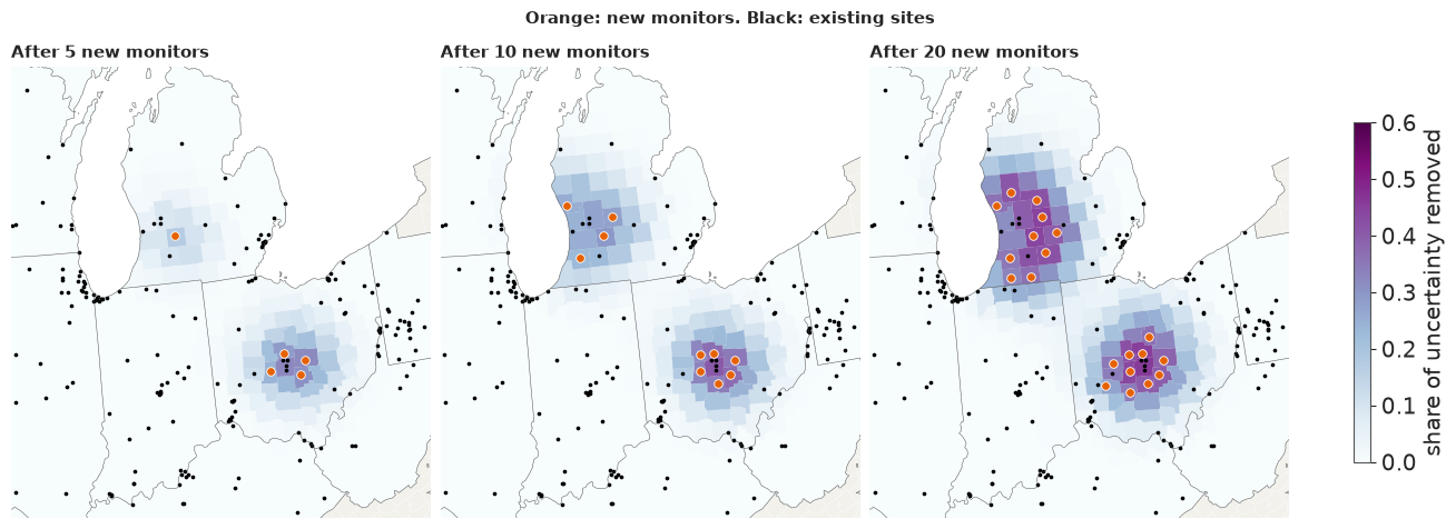
7 · How many monitors?
A greedy gain is exact only in the first round. After that the search keeps each draw's mean fixed, because the earlier readings are unknown, so the gains do not add up to "people moved". To get that number we value the set directly: simulate readings jointly at all the chosen sites, update every draw on all of them at once, and make the calls. We simulate one set of 20 readings and use the first $k$ for each size $k$, so sizes differ only by the sites added. The cell also values three rules of thumb and a noisier reading.
def joint_curve(field_, picks, sizes, sims=1500, seed=0, noise_scale=1.0):
    """Simulated gain of the first k picks, for each k in `sizes`: (sizes, sims) overall and in empty counties.

    The readings are nested. One set is drawn for the whole list, and a smaller set uses its first k. The
    lower Cholesky factor makes that exact, because its first k rows use only the first k normals.
    """
    check = np.random.default_rng(seed)
    picks = list(picks)[: max(sizes)]
    mu, noise = field_["means"].astype(float), field_["noise"] * noise_scale
    line, count = np.log(LINE), len(mu)
    rows_all = covariance_rows(field_, picks).astype(float)
    variance_ = (field_["eta2"][:, None] - (field_["half"] ** 2).sum(axis=1)).astype(float)
    lower = np.stack([linalg.cholesky(rows_all[i][:, picks] + noise[i] * np.eye(len(picks)), lower=True)
                      for i in range(count)])
    which = check.integers(count, size=sims)
    y = mu[which][:, picks] + np.einsum("sij,sj->si", lower[which], check.normal(size=(sims, len(picks))))
    p_before = ndtr((mu - line) / np.sqrt(variance_)).mean(axis=0)
    empty_people = population * ~monitored
    before = loss(p_before, population, "wrong"), loss(p_before, empty_people, "wrong")
    gains = np.empty((2, len(sizes), sims))
    for row, k in enumerate(sizes):
        root = lower[:, : k, : k]
        inverse = np.linalg.inv(root)
        half_log_det = np.log(np.diagonal(root, axis1=1, axis2=2)).sum(axis=1)
        solved = np.stack([linalg.cho_solve((root[i], True), rows_all[i, : k]) for i in range(count)])
        sd = np.sqrt(np.maximum(variance_ - (rows_all[:, : k] * solved).sum(axis=1), 1e-10))

        def after(s):
            gap = y[s, : k] - mu[:, picks[: k]]
            z = np.einsum("tij,tj->ti", inverse, gap)
            log = -0.5 * (z ** 2).sum(axis=1) - half_log_det
            w = np.exp(log - logsumexp(log))
            use = np.flatnonzero(w > 1e-6)
            p = w[use] @ ndtr((mu[use] + (gap[use][:, None] @ solved[use])[:, 0] - line) / sd[use])
            return loss(p, population, "wrong"), loss(p, empty_people, "wrong")

        with ThreadPoolExecutor(WORKERS) as pool:
            left = np.array(list(pool.map(after, range(sims))))
        gains[0, row], gains[1, row] = before[0] - left[:, 0], before[1] - left[:, 1]
    return gains[0], gains[1]


def joint_value(field_, picks, sims=800, seed=0, noise_scale=1.0):
    """What one set is worth: value and se, overall and in empty counties."""
    overall, in_empty = joint_curve(field_, picks, [len(picks)], sims, seed, noise_scale)
    root_n = np.sqrt(sims)
    return (float(overall.mean()), float(overall.std() / root_n), float(in_empty.mean()), float(in_empty.std() / root_n))


def rule_of_thumb(score, rounds=20):
    """Greedy on a simple score of the network, with no value of information."""
    network, picks = Network(field), []
    for _ in range(rounds):
        values = score(network).copy()
        values[picks] = -np.inf
        best = candidates[np.argmax(values[candidates])]
        picks.append(int(best))
        network.pick(int(best))
    return picks


def fog(network):
    """Posterior sd in µg/m³, the measure ranked in section 5, after the picks so far."""
    return np.exp(network.mu.mean(axis=0)) * np.sqrt(network.var.mean(axis=0) + network.mu.var(axis=0))


with stage("rules of thumb"):
    rules = {"Most uncertain": rule_of_thumb(fog),
             "Uncertainty x people": rule_of_thumb(lambda n: fog(n) * population),
             "Most populous empty": candidates[np.argsort(-population[candidates])][:20].tolist()}

with stage("joint value"):
    sizes = (1, 2, 3, 5, 8, 12, 16, 20)
    overall, in_empty = joint_curve(field, main["picks"], sizes)
    joint = pd.DataFrame({"joint": overall.mean(axis=1), "se": overall.std(axis=1) / np.sqrt(overall.shape[1]),
                          "in empty counties": in_empty.mean(axis=1)}, index=sizes)
    joint["sum of gains"] = np.cumsum(main["gains"])[np.array(sizes) - 1]
    joint["overstated by"] = joint["sum of gains"] / joint["joint"]
    per_rule = {name: [joint_value(field, picks[: k]) for k in (5, 20)] for name, picks in rules.items()}
    halves_value = [joint_value(field, picks) for picks in halves]
    between_windows = joint_value(field, main["picks"], noise_scale=1.2)
print((joint / [1e6, 1e6, 1e6, 1e6, 1]).round(3).to_string())
print(f"Worst overstatement here: {joint['overstated by'].max():.2f}x (2.1x across the pilot's draw sets)")
compare = pd.DataFrame({name: {"overlap with EVSI top 20": overlap(picks, main["picks"]),
                               "value of 5 (M)": values[0][0] / 1e6, "value of 20 (M)": values[1][0] / 1e6}
                        for (name, picks), values in zip(rules.items(), per_rule.values())}).T
compare.loc["EVSI, lazy greedy"] = [20, joint.loc[5, "joint"] / 1e6, joint.loc[20, "joint"] / 1e6]
print(compare.round(2).to_string())
print(f"Joint value of each half's 20 picks: {halves_value[0][0] / 1e6:.2f} and {halves_value[1][0] / 1e6:.2f} million "
      f"(se {halves_value[0][1] / 1e6:.2f})")
print(f"Reading noise variance 20% larger, for the gap between the window read and the window scored: "
      f"{between_windows[0] / 1e6:.2f} million (se {between_windows[1] / 1e6:.2f})")
print(f"Of the 20 picks' {joint.loc[20, 'joint'] / 1e6:.2f} million, {joint.loc[20, 'in empty counties'] / 1e6:.2f} million "
      f"falls in empty counties (se {in_empty[-1].std() / np.sqrt(in_empty.shape[1]) / 1e6:.2f}); "
      f"wrong-call people there now: {risk[~monitored].sum() / 1e6:.2f} million")
steps = pd.DataFrame({"from": sizes[:-1], "to": sizes[1:]})
per_step = np.diff(overall, axis=0) / np.diff(sizes)[:, None] / 1e3
steps["people per extra monitor (thousand)"] = per_step.mean(axis=1)
steps["se"] = per_step.std(axis=1) / np.sqrt(per_step.shape[1])
print(steps.round(1).to_string(index=False))
print(f"Monitors 12 to 20 add {(overall[-1] - overall[list(sizes).index(12)]).mean() / 1e6:.3f} million "
      f"(se {(overall[-1] - overall[list(sizes).index(12)]).std() / np.sqrt(overall.shape[1]) / 1e6:.3f}); the first five "
      f"do {joint.loc[5, 'joint'] / joint.loc[20, 'joint']:.0%} of the work of twenty")

fig, axes = plt.subplots(1, 2, figsize=(12, 4.6), width_ratios=[1.5, 1], layout="constrained")
ax = axes[0]
ax.plot(sizes, joint["sum of gains"] / 1e6, color=MUTED, ls="--", marker="o", ms=3,
        label="sum of greedy gains: do not read this as people")
ax.fill_between(sizes, (joint["joint"] - 2 * joint["se"]) / 1e6, (joint["joint"] + 2 * joint["se"]) / 1e6,
                color=BELOW, alpha=0.2, lw=0)
ax.plot(sizes, joint["joint"] / 1e6, color=BELOW, marker="o", ms=4, label="simulated joint value, 2 se band")
for (name, values), marker, nudge in zip(per_rule.items(), "s^D", (-0.3, 0, 0.3)):
    ax.scatter([5 + nudge, 20 + nudge], [v[0] / 1e6 for v in values], marker=marker, s=38, c=PICK, label=name, zorder=3)
ax.set_xticks([1, 5, 10, 15, 20])
ax.set(xlabel="monitors funded", ylabel="people moved to a right call (million)")
ax.set_title("What a set of monitors is worth", fontsize=11)
ax.legend(fontsize=8, loc="upper left")
ax = axes[1]
middle = (steps["from"] + steps["to"]) / 2
ax.bar(middle, steps["people per extra monitor (thousand)"], width=np.diff(sizes) * 0.85, color=BELOW, alpha=0.75,
       yerr=2 * steps["se"], ecolor="k", error_kw={"lw": 0.8})
ax.axhline(0, color="k", lw=0.8)
ax.set_xticks([1, 5, 10, 15, 20])
ax.set(xlabel="monitors funded", ylabel="people per extra monitor (thousand)")
ax.set_title("Set your own line here. Black bars: 2 se of each step", fontsize=11);
    joint     se  in empty counties  sum of gains  overstated by
1   0.139  0.008             -0.003         0.143          1.025
2   0.202  0.010             -0.003         0.266          1.316
3   0.249  0.012             -0.001         0.381          1.530
5   0.372  0.018             -0.004         0.596          1.601
8   0.473  0.022              0.005         0.878          1.856
12  0.580  0.025              0.006         1.200          2.070
16  0.654  0.027              0.008         1.475          2.256
20  0.731  0.028              0.015         1.720          2.354
Worst overstatement here: 2.35x (2.1x across the pilot's draw sets)
                      overlap with EVSI top 20  value of 5 (M)  value of 20 (M)
Most uncertain                             0.0            0.04             0.09
Uncertainty x people                       3.0            0.07             0.54
Most populous empty                        3.0            0.11             0.56
EVSI, lazy greedy                         20.0            0.37             0.73
Joint value of each half's 20 picks: 0.77 and 0.69 million (se 0.04)
Reading noise variance 20% larger, for the gap between the window read and the window scored: 0.67 million (se 0.04)
Of the 20 picks' 0.73 million, 0.02 million falls in empty counties (se 0.01); wrong-call people there now: 1.15 million
 from  to  people per extra monitor (thousand)  se
    1   2                                 62.5 5.7
    2   3                                 47.0 7.9
    3   5                                 61.6 6.9
    5   8                                 33.7 4.4
    8  12                                 26.6 3.3
   12  16                                 18.6 3.0
   16  20                                 19.3 2.6
Monitors 12 to 20 add 0.151 million (se 0.016); the first five do 51% of the work of twenty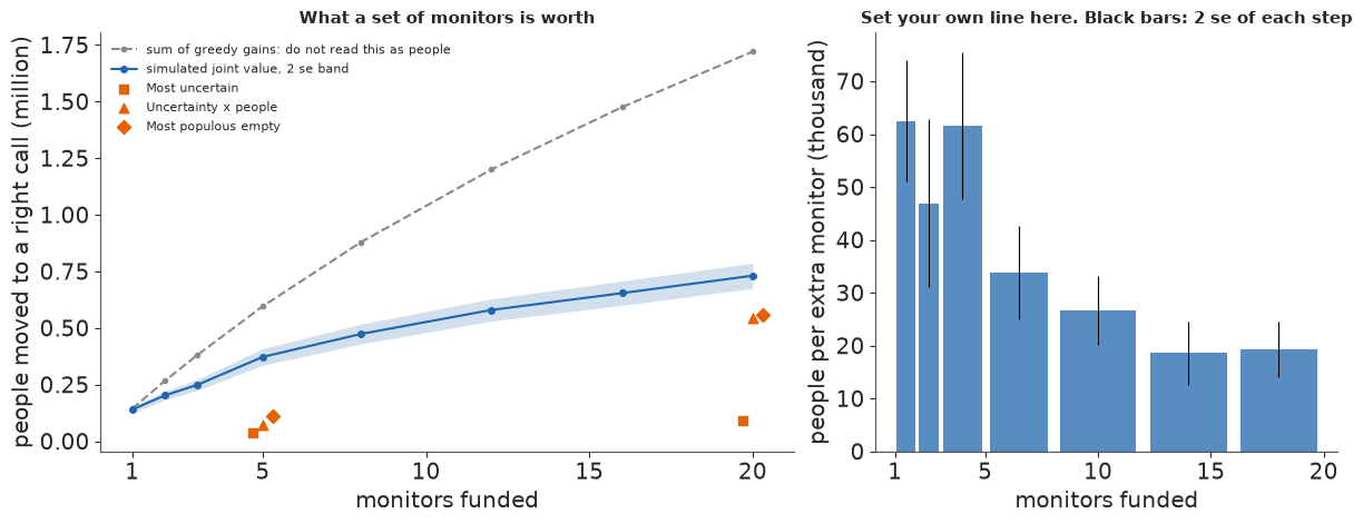
Failure 3: summed gains are not people
The dashed line adds up greedy gains: about 1.7 million people at 20 monitors. The simulation says 0.73 million. The sum overstates by about 2.4 times (1.7-2.4 over several runs), so only the first monitor's gain is safe to quote. On a disjoint set of draws the same list is worth about 1.0 million (section 8), so call it 0.7-1.0 million for twenty monitors. Other runs have valued it as high as 1.2 million.
When to stop is the right-hand panel. We have no sourced cost for a monitor, so the planner draws the line, in people per monitor. The first monitor moves about 140 thousand people, the next few about 50-60 thousand each, monitors five to twelve about 30 thousand and twelve to twenty about 20 thousand. The first five do about half the work of twenty, but the curve never reaches zero: monitors 12 to 20 still add 0.15 million people (se 0.02). There is no natural stopping point.
Against the rules of thumb, at five monitors EVSI is worth three to five times the two sensible rules (uncertainty times people; most populous empty counties) and nine times "most uncertain". At twenty the sensible rules recover about three quarters of the value, because any list that crowds into populous near-line areas finds some. The uncertainty rule never does.
The window gap. Year effects have an sd of about 0.1 on the log scale, so a later three-year mean drifts by about 0.05, which raises the reading noise variance by about a fifth. With that noise the list loses less than a tenth of its value (0.67 million).
Almost none of the value lands in empty counties: 0.02 million (se 0.01) of the 0.73, where 1.15 million people are at risk. The rest is a firmer read on counties that already have monitors.
Failure 4: the search's shortcut bends the picks
After a pick, a county's variance shrinks but its mean stays put, so a county near 0.5 keeps drawing picks when half the possible readings would have settled it. The search misjudges which sets are worth most, not only how much.
The fix is to score what a set leaves behind. For one Gaussian county $j$, readings at a set of sites move its mean by a normal amount whose variance $u_j$ adds up pick by pick. With $m_j$ the county's mean distance from the line on the log scale and $s_j^2$ its total variance, the expected loss after the set is a one-dimensional integral,
$$\text{people}_j\;\mathbb{E}_{z}\big[\min(p_j, 1 - p_j)\big], \qquad p_j = \Phi\!\left(\frac{m_j + z\sqrt{u_j}}{\sqrt{s_j^2 - u_j}}\right), \quad z \sim \text{Normal}(0, 1),$$
summed over counties. The moving-means search below uses that score, with the draws pooled into
one mean and variance per county. joint_curve then values its list exactly as it valued the first.
class JointNetwork(Network):
    """A search that scores what a set leaves behind, with each county's mean free to move.

    For one Gaussian county, readings at a set of sites move its mean by a normal amount, with a
    variance that adds up pick by pick, and the expected loss is then a one-dimensional integral that
    adds across counties. Draws are pooled into one mean and variance per county, and covariances come
    from every fifth draw. This is a score for the search and not a value: `joint_curve` measures sets.
    """

    def __init__(self, field_, every=5, **options):
        super().__init__(field_, keep=slice(None, None, every), **options)
        means = field_["means"][:, self.where]
        variance_ = field_["eta2"][:, None] - (field_["half"][:, :, self.where] ** 2).sum(axis=1)
        self.m = means.mean(axis=0) - self.line
        self.total = variance_.mean(axis=0) + means.var(axis=0)
        self.moved = np.zeros_like(self.total)
        self.z = np.float32(ndtri((np.arange(32) + 0.5) / 32))[:, None]

    def left(self, slots, moved):
        moved = np.minimum(moved, 0.9999 * self.total[slots])
        p = ndtr((self.m[slots] + self.z * np.sqrt(moved)) / np.sqrt(self.total[slots] - moved))
        return loss(p, self.weight[self.where[slots]], self.objective).mean()

    def shift(self, c, slots):
        """How much a reading at `c` adds to the variance of each county's mean."""
        cross = self.block[:, CANDIDATE_ROW[c]][:, slots]
        if self.k:
            cross = cross - (self.u[:, : self.k, c][:, None] @ self.u[:, : self.k][:, :, self.where[slots]])[:, 0]
        return (cross ** 2 / (self.var[:, c] + self.noise)[:, None]).mean(axis=0)

    def reach_of(self, c):
        return np.flatnonzero(gap32[c, self.where] < self.radius)

    def value(self, c):
        slots = self.reach_of(c)
        if slots.size == 0:
            return 0.0
        return float(self.left(slots, self.moved[slots]) - self.left(slots, self.moved[slots] + self.shift(c, slots)))

    def pick(self, c):
        slots = self.reach_of(c)
        self.moved[slots] += self.shift(c, slots)
        super().pick(c)


def nearest_gap(picks):
    """Median km from each pick to the nearest other pick."""
    gaps = gap_county[np.ix_(picks, picks)] + np.diag(np.full(len(picks), np.inf))
    return float(np.median(gaps.min(axis=1)))


with stage("search with moving means"):
    spread = lazy_greedy(JointNetwork(field), top=len(candidates))["picks"]
with stage("joint value"):
    spread_overall, spread_in_empty = joint_curve(field, spread, (5, 20))
print("The moving-means list:", ", ".join(short_name[spread]))
print(f"Shares {overlap(spread, main['picks'])} of 20 with the fixed-means list; states "
      f"{pd.Series(table['state'].to_numpy()[spread]).value_counts().to_dict()}; median km to the nearest other pick "
      f"{nearest_gap(spread):.0f}, against {nearest_gap(main['picks']):.0f}")
root_n = np.sqrt(overall.shape[1])
for row, k in enumerate((5, 20)):
    fixed_list = overall[sizes.index(k)]
    gap_ = spread_overall[row].mean() - fixed_list.mean()
    gap_se = np.sqrt(spread_overall[row].var() + fixed_list.var()) / root_n
    print(f"Joint value of {k:2d}: fixed means {fixed_list.mean() / 1e6:.2f}, moving means "
          f"{spread_overall[row].mean() / 1e6:.2f} million (difference {gap_ / 1e6:.2f}, se {gap_se / 1e6:.2f})")
print(f"Of the moving-means list's {spread_overall[1].mean() / 1e6:.2f} million, {spread_in_empty[1].mean() / 1e6:.2f} "
      f"million falls in empty counties (se {spread_in_empty[1].std() / root_n / 1e6:.2f})")
The moving-means list: Delaware OH, Barry MI, Madison OH, Harvey KS, Cass MI, Fairfield OH, Wood OH, Ionia MI, Greene OH, Licking OH, Muskegon MI, Butler KS, St. Joseph MI, Union OH, Boone IN, Livingston MI, Lapeer MI, Shiawassee MI, Pickaway OH, Van Buren MI
Shares 13 of 20 with the fixed-means list; states {'Michigan': 9, 'Ohio': 8, 'Kansas': 2, 'Indiana': 1}; median km to the nearest other pick 43, against 40
Joint value of  5: fixed means 0.37, moving means 0.42 million (difference 0.04, se 0.03)
Joint value of 20: fixed means 0.73, moving means 0.91 million (difference 0.18, se 0.04)
Of the moving-means list's 0.91 million, 0.03 million falls in empty counties (se 0.01)
The moving-means list is worth a fifth to a quarter more at twenty monitors: 0.91 million against 0.73 here (difference 0.18, se 0.04). At five the gain is small, 0.42 against 0.37 (se 0.03). It shares 13 picks with the first list, keeps most of Columbus and lower Michigan, and adds two Kansas counties near Wichita and one in Indiana. Its score is crude, so treat it as a better list, not the best one. The clusters survive (median gap to the nearest other pick 43 km against 40), and it puts no more of its value in empty counties, about 0.03 million.
8 · Whose objective, which standard, which sites?
The objective is a choice. "Fewest people on the wrong side" weighs a missed exceedance and a false one equally, and a state may not want to find exceedances at all. Keeping the call at p = 0.5, we change what counts as loss: missed exceedances only, false exceedances only, every county counting once, and only people in empty counties. Then we repeat the search at the old standard of 12.0, which few counties are anywhere near.
with stage("objectives"):
    runs = {"People": main["picks"],
            "Missed exceedances": lazy_greedy(Network(field, objective="missed"))["picks"],
            "False exceedances": lazy_greedy(Network(field, objective="false"))["picks"],
            "Counties, unweighted": lazy_greedy(Network(field, weight=np.ones(len(table))))["picks"],
            "People in empty counties": lazy_greedy(Network(field, weight=population * ~monitored))["picks"],
            "People, 12.0 standard": lazy_greedy(Network(field, line=12.05))["picks"]}
twelve = Network(field, line=12.05)
print(f"At 12.05: {twelve.open.sum()} undecided counties ({', '.join(short_name[twelve.open])}), "
      f"{loss(twelve.p, twelve.weight, 'wrong') / 1e6:.2f} million "
      f"people at risk of a wrong call; {len(runs['People, 12.0 standard'])} picks before value ran out")
for name, picks in runs.items():
    print(f"{name:24s} shares {overlap(picks, main['picks']):2d} with People; states "
          f"{pd.Series(table['state'].to_numpy()[picks]).value_counts().head(3).to_dict()}")

close = np.flatnonzero((p_now > 0.4) & (p_now < 0.6))
print("Counties with P(above) of 0.4-0.6:",
      ", ".join(f"{short_name[i]} {p_now[i]:.2f}" for i in close[np.argsort(-population[close])]))
empty_value = joint_value(field, runs["People in empty counties"])
print(f"20 picks made for empty counties: {empty_value[2] / 1e6:.2f} million people moved there "
      f"(se {empty_value[3] / 1e6:.2f}), {empty_value[0] / 1e6:.2f} million overall")

labels = list(runs)
every = sorted({c for picks in runs.values() for c in picks},
               key=lambda c: (table["state"].iloc[c], -sum(c in p for p in runs.values())))
fig, ax = plt.subplots(figsize=(8.2, 0.17 * len(every) + 1.8), layout="constrained")
for x, name in enumerate(labels):
    for y_, c in enumerate(every):
        if c in runs[name]:
            ax.scatter(x, y_, s=34, c=BELOW, lw=0)
ax.set_xticks(range(len(labels)), [t.replace(", ", ",\n").replace(" ", "\n", 1) for t in labels], fontsize=8)
ax.set_yticks(range(len(every)), short_name[every], fontsize=7.5)
ax.set(ylim=(len(every) - 0.5, -0.5))
ax.set_title("Every pick of every objective, one row per county, grouped by state", fontsize=11)
ax.grid(True, lw=0.3);
At 12.05: 1 undecided counties (Lincoln MT), 0.00 million people at risk of a wrong call; 1 picks before value ran out
People                   shares 20 with People; states {'Ohio': 10, 'Michigan': 10}
Missed exceedances       shares  0 with People; states {'Kansas': 10, 'Missouri': 7, 'Indiana': 1}
False exceedances        shares 12 with People; states {'Ohio': 15, 'Michigan': 5}
Counties, unweighted     shares 11 with People; states {'Michigan': 11, 'Indiana': 4, 'Ohio': 3}
People in empty counties shares  1 with People; states {'Indiana': 11, 'Michigan': 4, 'North Dakota': 1}
People, 12.0 standard    shares  0 with People; states {'Montana': 1}
Counties with P(above) of 0.4-0.6: Franklin OH 0.52, Kent MI 0.51, Montgomery OH 0.44, Sedgwick KS 0.43, Lake IN 0.41, Lucas OH 0.48, Hamilton IN 0.55, St. Joseph IN 0.54, Kalamazoo MI 0.55, Elkhart IN 0.47, Hendricks IN 0.42
20 picks made for empty counties: 0.06 million people moved there (se 0.02), 0.42 million overall
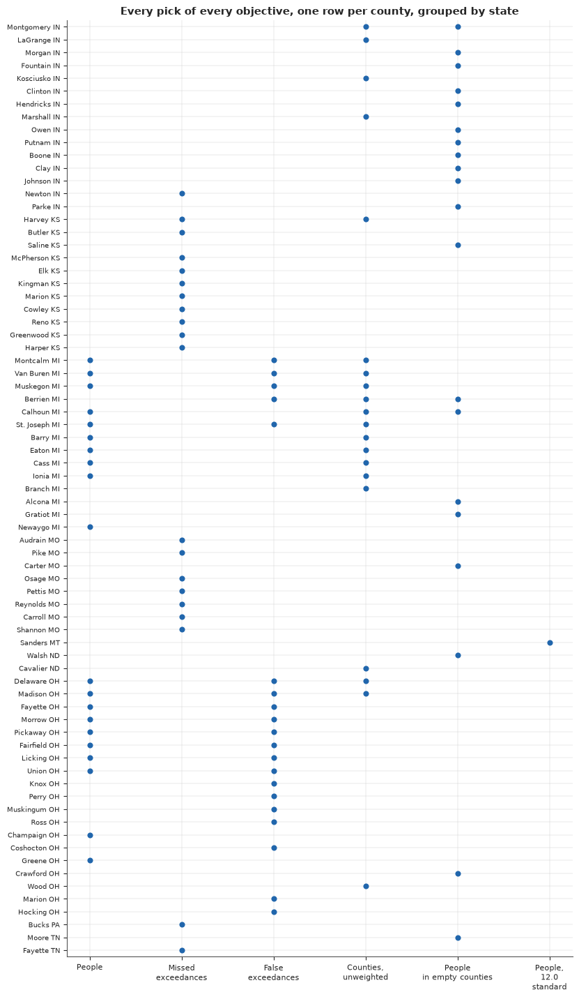
The list depends heavily on the objective. False exceedances keeps 12 of the 20 picks and stays in Ohio and Michigan. Unweighted counties keeps 11 and moves towards Michigan and Indiana. Missed exceedances keeps none. It pays for pushing a county just below 0.5 over the line, so it goes wherever such counties are: Kansas and Missouri here, with Sedgwick KS at 0.43 the kind of county it hunts. On another run it went to Indiana, Michigan and Illinois. People in empty counties, the objective closest to the planner's words, keeps one pick and moves about half the list to the counties around Indianapolis. Its prize is small: about 0.06 million people moved in empty counties (se 0.02), of 1.15 million at risk there. The 12.0 standard has one undecided county in the crop, Lincoln MT, and one pick before value runs out, so there is no shortlist to make.
A second draw set, and the excluded sites
Two more runs, each searched both ways. One uses a disjoint set of 200 draws from the same fit, which measures draw noise at the size we use. The other refits without the 15 crop sites excluded from comparison with the annual standard. They measure real air, so they stay in by default, but some may sit beside sources.
main_field_rows = {"fixed-means list": (joint.loc[20, "joint"], joint.loc[20, "se"]),
                   "moving-means list": (spread_overall[1].mean(), spread_overall[1].std() / root_n)}
main_field_rows |= {"fixed, searched here": main_field_rows["fixed-means list"],
                    "moving, searched here": main_field_rows["moving-means list"]}
worth = {"these 200 draws": main_field_rows}
del net, twelve, field
main.pop("network")
gc.collect()


def on_field(other):
    """Search both ways on another field, then value the main lists and its own lists there."""
    fixed = lazy_greedy(Network(other))["picks"]
    moving = lazy_greedy(JointNetwork(other), top=len(candidates))["picks"]
    named = {"fixed-means list": main["picks"], "moving-means list": spread,
             "fixed, searched here": fixed, "moving, searched here": moving}
    return fixed, moving, {name: joint_value(other, picks, seed=1)[:2] for name, picks in named.items()}


with stage("second draw set"):
    field_two = make_field(d, fit, shift=5)
    second, spread_second, worth["a disjoint 200 draws"] = on_field(field_two)
    del field_two
    gc.collect()
print(f"Top 20, two disjoint sets of 200 draws: {overlap(main['picks'], second)} in common; "
      f"moving-means search: {overlap(spread, spread_second)}")

excluded = set(checks["excluded_sites"])
kept = crop_sites[~crop_sites["site"].isin(excluded)].reset_index(drop=True)
print(f"{len(excluded)} excluded sites in the contiguous US, {len(crop_sites) - len(kept)} in the crop: "
      f"refit on {len(kept)} sites")
d_drop = design(kept)
with stage("refit without excluded sites"):
    idata_drop = fit_m1(d_drop, RANDOM_SEED + 1)
summary_drop = az.summary(idata_drop, var_names=list(NAMES), ci_prob=0.9, ci_kind="eti", round_to=3)
print(summary_drop.loc[["eta", "ell"]].to_string())
print(f"max r_hat {summary_drop['r_hat'].astype(float).max():.3f}; "
      f"divergences {int(idata_drop.sample_stats['diverging'].sum())}")
fit_drop = draws_of(idata_drop)
del idata_drop
gc.collect()
with stage("county conditionals, greedy without excluded sites"):
    field_drop = make_field(d_drop, fit_drop)
    p_drop = Network(field_drop).p.copy()
    dropped, spread_dropped, worth["no excluded sites"] = on_field(field_drop)
    del field_drop
    gc.collect()
gap_lists = gap_county[np.ix_(dropped, main["picks"])]
print(f"Top 20 with and without them: {overlap(main['picks'], dropped)} in common; "
      f"{(gap_lists.min(axis=1) < 100).mean():.0%} of the new picks lie within 100 km of a kept pick; "
      f"moving-means search: {overlap(spread, spread_dropped)} in common")
print("States, fixed means:", pd.Series(table["state"].to_numpy()[dropped]).value_counts().to_dict())
print("States, moving means:", pd.Series(table["state"].to_numpy()[spread_dropped]).value_counts().to_dict())
print(f"Mean |change in P(above)| {np.abs(p_now - p_drop).mean():.3f}; 99th percentile "
      f"{np.quantile(np.abs(p_now - p_drop), 0.99):.3f}; counties changing side of 0.5: "
      f"{((p_now > 0.5) != (p_drop > 0.5)).sum()}")
print("Change side:", ", ".join(f"{short_name[i]} {p_now[i]:.2f} to {p_drop[i]:.2f}"
                                for i in np.flatnonzero((p_now > 0.5) != (p_drop > 0.5))))
Top 20, two disjoint sets of 200 draws: 18 in common; moving-means search: 19
30 excluded sites in the contiguous US, 15 in the crop: refit on 404 sites
        mean      sd  eti90_lb  eti90_ub  ess_bulk  ess_tail  r_hat  mcse_mean  mcse_sd
eta    0.222   0.041     0.168     0.296  1717.799  1380.310  0.999      0.001    0.001
ell  350.169  83.959   241.285   500.012  1383.455  1246.699  0.999      2.366    2.737
max r_hat 1.005; divergences 0
Top 20 with and without them: 11 in common; 85% of the new picks lie within 100 km of a kept pick; moving-means search: 12 in common
States, fixed means: {'Michigan': 16, 'Illinois': 2, 'Wisconsin': 1, 'Ohio': 1}
States, moving means: {'Michigan': 8, 'Ohio': 8, 'Illinois': 4}
Mean |change in P(above)| 0.010; 99th percentile 0.141; counties changing side of 0.5: 6
Change side: Kalamazoo MI 0.55 to 0.48, St. Joseph IN 0.54 to 0.38, Hamilton IN 0.55 to 0.36, Franklin OH 0.52 to 0.37, Kent MI 0.51 to 0.48, Lincoln MT 0.68 to 0.43
Two disjoint sets of 200 draws share 18 of 20 picks, and the moving-means search 19: that is draw
noise at the size we use. Dropping the excluded sites keeps the fit clean and moves ell from about
310 to 350 km, but the first list keeps only 11 of its 20 picks: more than draw noise. Most of
its Ohio picks go and Michigan takes 16 places, so "85% within 100 km of a kept pick" flatters it,
since the one kept pick at Delaware OH sits near the whole Ohio ring. The moving-means list holds up
better, keeping 12 picks, its Ohio ones among them. Six counties change side of 0.5, Franklin OH
among them; one of Franklin's four sites, the one reading 9.86, is excluded. We did not isolate
which sites drive the move; whether to keep them depends on why each was excluded.
The method term, against the instruments themselves
Section 2 flagged the method term, which the model learns across sites and which can absorb rural air. There is a direct check: where an FRM filter and a continuous instrument ran at the same site on the same day, they saw the same air, and their ratio measures the instrument alone. We refit with the pairs as the prior on the method term and search both ways on the new field.
print(f"BAM sites: mean {crop_sites.loc[crop_sites['share_BAM'] > 0.5, 'mean'].mean():.1f} {UG}, mean log density "
      f"{crop_sites.loc[crop_sites['share_BAM'] > 0.5, 'log_density'].mean():.1f}; all other sites "
      f"{crop_sites.loc[crop_sites['share_BAM'] <= 0.5, 'mean'].mean():.1f} {UG}, "
      f"{crop_sites.loc[crop_sites['share_BAM'] <= 0.5, 'log_density'].mean():.1f}")
pairs_table = pd.DataFrame(checks["paired_method"]).T[["sites", "site_days", "mean", "se"]]
pairs_table["model"] = summary.loc[[f"beta_method[{m}]" for m in pairs_table.index], "mean"].astype(float).to_numpy()
print(pairs_table.round(3).to_string())

prior_mean = pairs_table.loc[list(METHODS), "mean"].to_numpy(float)
prior_sd = np.maximum(pairs_table.loc[list(METHODS), "se"].to_numpy(float), 0.01)
with stage("refit with paired method prior"):
    idata_pair = fit_m1(d, RANDOM_SEED + 2, method_prior=(prior_mean, prior_sd))
summary_pair = az.summary(idata_pair, var_names=list(NAMES), ci_prob=0.9, ci_kind="eti", round_to=3)
print(summary_pair.filter(like="beta_method", axis=0)[["mean", "sd"]].to_string())
print(f"max r_hat {summary_pair['r_hat'].astype(float).max():.3f}; "
      f"min bulk ESS {summary_pair['ess_bulk'].astype(float).min():.0f}; "
      f"divergences {int(idata_pair.sample_stats['diverging'].sum())}")
fit_pair = draws_of(idata_pair)
del idata_pair
gc.collect()
with stage("county conditionals, greedy with paired prior"):
    field_pair = make_field(d, fit_pair)
    p_pair = Network(field_pair).p.copy()
    risk_pair = population * np.minimum(p_pair, 1 - p_pair)
    paired_list, spread_paired, worth["paired method prior"] = on_field(field_pair)
    del field_pair
    gc.collect()
print(f"With the paired prior: {risk_pair.sum() / 1e6:.2f} million at risk (was {risk.sum() / 1e6:.2f}), "
      f"{risk_pair[~monitored].sum() / 1e6:.2f} in empty counties (was {risk[~monitored].sum() / 1e6:.2f}); "
      f"{((p_pair > 0.01) & (p_pair < 0.99)).sum()} undecided (was {undecided.sum()}); "
      f"{(p_pair > 0.5).sum()} called above, {population[p_pair > 0.5].sum() / 1e6:.1f} million people "
      f"(was {(p_now > 0.5).sum()}, {population[p_now > 0.5].sum() / 1e6:.1f})")
moved_side = np.flatnonzero((p_now > 0.5) != (p_pair > 0.5))
print("Change side:", ", ".join(f"{short_name[i]} {p_now[i]:.2f} to {p_pair[i]:.2f}" for i in moved_side))
print(f"Top 20 against the main list: fixed means {overlap(main['picks'], paired_list)} of 20, "
      f"moving means {overlap(spread, spread_paired)} of 20")
print("States, fixed means:", pd.Series(table["state"].to_numpy()[paired_list]).value_counts().to_dict())
print("States, moving means:", pd.Series(table["state"].to_numpy()[spread_paired]).value_counts().to_dict())
print(pd.DataFrame({field_name: {list_name: f"{value / 1e6:.2f} ({se / 1e6:.2f})" for list_name, (value, se) in row.items()}
                    for field_name, row in worth.items()}).T.to_string())
BAM sites: mean 6.2 µg/m³, mean log density 3.1; all other sites 8.0 µg/m³, 4.8
       sites  site_days   mean     se  model
T640   114.0    34684.0  0.063  0.007  0.033
BAM     20.0     4767.0 -0.035  0.017 -0.111
other    8.0     1689.0  0.027  0.040  0.007
mean sd beta_method[T640] 0.063 0.010 beta_method[BAM] -0.051 0.014 beta_method[other] 0.034 0.029 max r_hat 1.007; min bulk ESS 1377; divergences 0
With the paired prior: 7.36 million at risk (was 10.43), 0.44 in empty counties (was 1.15); 259 undecided (was 452); 2 called above, 1.0 million people (was 9, 10.9)
Change side: Kalamazoo MI 0.55 to 0.37, St. Joseph IN 0.54 to 0.31, Hamilton IN 0.55 to 0.26, Franklin OH 0.52 to 0.35, Kent MI 0.51 to 0.32, Wayne MI 0.70 to 0.44, Cook IL 0.74 to 0.50
Top 20 against the main list: fixed means 0 of 20, moving means 12 of 20
States, fixed means: {'Illinois': 5, 'Michigan': 4, 'Missouri': 3, 'Iowa': 3, 'Nebraska': 2, 'Wisconsin': 1, 'Indiana': 1, 'Kansas': 1}
States, moving means: {'Michigan': 8, 'Ohio': 7, 'Illinois': 4, 'Wisconsin': 1}
                     fixed-means list moving-means list fixed, searched here moving, searched here
these 200 draws           0.73 (0.03)       0.91 (0.03)          0.73 (0.03)           0.91 (0.03)
a disjoint 200 draws      0.97 (0.05)       1.20 (0.05)          0.99 (0.05)           1.17 (0.05)
no excluded sites         0.73 (0.04)       0.90 (0.04)          0.92 (0.04)           0.90 (0.04)
paired method prior       0.31 (0.02)       0.37 (0.02)          0.36 (0.02)           0.57 (0.02)
BAM sites are cleaner (6.2 against 8.0 µg/m³) and much less crowded than the rest, and the across-site term puts BAM about 10% low where the pairs say about 3%. For T640, the most common instrument, it goes the other way: +3% in the model, +6% in the pairs. Of the checks in this section, this disagreement moves the totals and the values most. With the paired prior the fit stays clean. About 7.4 million people are at risk instead of 10, 0.4 million rather than 1.15 in empty counties, and 259 counties are undecided instead of 452. Only 2 counties are called above: Franklin OH, Wayne MI and Kent MI cross below, and Cook IL lands on the line at 0.50, so the people in counties called above swing between about 1 and 6 million on that one call.
The lists move too. The first search on the new field shares none of its picks with its main list (0-7 across fits); the moving-means search keeps 12. In the last table (millions, se in brackets) the first two columns score the two main lists on each field: on the second draw set the moving-means list is worth 1.2 million, the first list 1.0, and on the paired field they are worth only 0.37 and 0.31. The last two columns value lists searched afresh on each field. The moving-means search wins on the second draw set and with the paired prior (0.57 against 0.36, though the two have come out level at about 0.5 on another run). Without the excluded sites the two are level.
We keep the learned term in the main run, because the pairs come from selected sites on FRM sampling days and this is one refit. But the 10 million is not settled.
9 · The band
The answer is a band of places, built from four lists, all from the moving-means search, since its main list scored higher on all four fields and kept more of its picks when the field changed. Two lists are the two draw sets of the main fit, so draw noise counts once; the other two drop the excluded sites or use the paired method prior. A county's standing is how many of the four picked it. The table is sorted by place, because the data do not support a rank, and the first search's lists are printed by state to show the instability the band absorbs.
lists = {"these draws": spread, "other draws": spread_second, "no excluded sites": spread_dropped,
         "paired method prior": spread_paired}
ASSUMPTIONS = len(lists)
count = pd.Series([c for picks in lists.values() for c in picks]).value_counts()
band = pd.DataFrame({"county": short_name[count.index], "state": table["state"].to_numpy()[count.index],
                     "lists": count.to_numpy(), "people": population[count.index].round(-3).astype(int),
                     "P(above)": p_now[count.index].round(2),
                     "km to nearest monitor": distance(xy_county[count.index], d["xy"]).min(axis=1).round(0).astype(int)},
                    index=count.index)
core = band[band["lists"] >= 3]
print(f"{len(band)} counties on at least one list; {len(core)} on at least 3 of {ASSUMPTIONS}; "
      f"{(band['lists'] == ASSUMPTIONS).sum()} on all {ASSUMPTIONS}")
print(core.sort_values(["state", "county"]).to_string(index=False))
print(band.groupby("state")["lists"].agg(["size", "sum"]).sort_values("sum", ascending=False).to_string())
print("Fixed-means lists, for comparison:")
for name, picks in {"these draws": main["picks"], "other draws": second, "half A": halves[0], "half B": halves[1],
                    "no excluded sites": dropped, "paired method prior": paired_list}.items():
    print(f"  {name:20s}{pd.Series(table['state'].to_numpy()[picks]).value_counts().head(4).to_dict()}")

with stage("random sets from the band"):
    field = make_field(d, fit)
    picker = np.random.default_rng(RANDOM_SEED)
    samples = [joint_value(field, picker.choice(band.index.to_numpy(), 20, replace=False).tolist(), sims=400)[0]
               for _ in range(6)]
    del field
    gc.collect()
print(f"Six random sets of 20 from the band: {min(samples) / 1e6:.2f}-{max(samples) / 1e6:.2f} million "
      f"(moving-means list {spread_overall[1].mean() / 1e6:.2f}, fixed-means list {joint.loc[20, 'joint'] / 1e6:.2f})")

for_empty = runs["People in empty counties"]
places = xy_county[band.index[band["lists"] >= 2]]
fig, ax = plt.subplots(figsize=(12, 7.2), layout="constrained")
shapes = paint(ax, p_now, CLOSE_CALL, Normalize(0, 1))
shapes.set_alpha(0.5)
ax.scatter(crop_sites["x_km"], crop_sites["y_km"], s=6, c="#333333", lw=0, label="existing site")
ax.scatter(xy_county[for_empty, 0], xy_county[for_empty, 1], s=70, marker="s", facecolor="none", edgecolor=BELOW, lw=1.4,
           label="a pick when only empty counties count")
ax.scatter(xy_county[band.index, 0], xy_county[band.index, 1], s=band["lists"] ** 2 * 12, c=band["lists"], cmap="YlOrRd",
           norm=Normalize(0, ASSUMPTIONS), edgecolor="k", lw=0.5, zorder=3)
for size in range(1, ASSUMPTIONS + 1):
    ax.scatter([], [], s=size ** 2 * 12, color=plt.get_cmap("YlOrRd")(size / ASSUMPTIONS), edgecolor="k", lw=0.5,
               label=f"on {size} of {ASSUMPTIONS} lists")
labelled = band.index[band["lists"] >= 3]
for turn, i in enumerate(labelled[np.argsort(xy_county[labelled, 1])]):
    dx, dy = ((-9, -9), (9, -9), (-9, 9), (9, 9))[turn % 4]
    ax.annotate(short_name[i].rsplit(" ", 1)[0], xy_county[i], xytext=(dx, dy), textcoords="offset points", fontsize=7.5,
                ha="right" if dx < 0 else "left", va="center",
                path_effects=[pe.withStroke(linewidth=2, foreground="w")], zorder=4)
ax.set(xlim=(places[:, 0].min() - 330, places[:, 0].max() + 150), ylim=(places[:, 1].min() - 150, places[:, 1].max() + 130))
ax.legend(loc="upper left", bbox_to_anchor=(1.0, 1.0), frameon=True, fontsize=9)
ax.set_title("The shortlist is a band of places. Larger, darker circles survive more of the checks",
             loc="left", fontsize=11);
32 counties on at least one list; 15 on at least 3 of 4; 9 on all 4
       county    state  lists  people  P(above)  km to nearest monitor
     Barry MI Michigan      4   64000      0.17                     40
      Cass MI Michigan      4   52000      0.14                     26
     Ionia MI Michigan      3   66000      0.12                     47
    Lapeer MI Michigan      3   89000      0.02                     34
Livingston MI Michigan      3  197000      0.15                     43
  Muskegon MI Michigan      3  177000      0.09                     49
St. Joseph MI Michigan      3   61000      0.19                     44
 Van Buren MI Michigan      3   76000      0.18                     38
  Delaware OH     Ohio      4  238000      0.13                     12
 Fairfield OH     Ohio      4  168000      0.03                     31
   Licking OH     Ohio      4  185000      0.03                     37
   Madison OH     Ohio      4   46000      0.01                     31
  Pickaway OH     Ohio      4   62000      0.01                     27
     Union OH     Ohio      4   72000      0.04                     27
      Wood OH     Ohio      4  133000      0.08                     19
           size  sum
state
Michigan     14   34
Ohio          9   31
Illinois      5    8
Kansas        2    4
Indiana       1    2
Wisconsin     1    1
Fixed-means lists, for comparison:
  these draws         {'Ohio': 10, 'Michigan': 10}
  other draws         {'Michigan': 11, 'Ohio': 9}
  half A              {'Michigan': 11, 'Ohio': 9}
  half B              {'Ohio': 11, 'Michigan': 9}
  no excluded sites   {'Michigan': 16, 'Illinois': 2, 'Wisconsin': 1, 'Ohio': 1}
  paired method prior {'Illinois': 5, 'Michigan': 4, 'Missouri': 3, 'Iowa': 3}
Six random sets of 20 from the band: 0.81-0.88 million (moving-means list 0.91, fixed-means list 0.73)
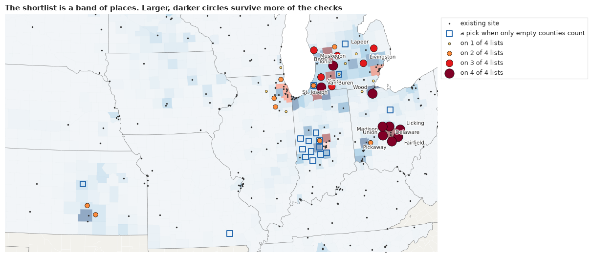
Thirty-two counties appear on at least one list. Fifteen are on at least three of the four, and 9 are on all four: Delaware, Fairfield, Licking, Madison, Pickaway and Union around Columbus, Wood in north-west Ohio, and Barry and Cass in lower Michigan. Those 9 are the robust core; the rest depend on which draws, which sites and which method prior we accept. The first search's lists show how much: dropping the excluded sites takes Ohio from half of its list to a single pick.
Random sets of 20 from the band are worth 0.81-0.88 million, a little below the moving-means list (0.91) and above the first list (0.73). So a planner who picks any 20 from around these places is close to the best this analysis found. Six random sets is a small test, so that is a rough statement, not a guarantee. The blue squares are the picks when only empty counties count, a different answer.
So the planner should not fund "where we are most uncertain". For a firmer read on exposure across the populated Midwest, the band around Columbus and lower Michigan is the answer; to resolve calls in empty counties, the list moves towards Indianapolis and the gain is far smaller. Settle the method term before buying anything: it costs no monitors, moves the number at risk by about 3 million and cuts the lists' value by half or more. Buy in stages from the band, rescoring each stage. And check the band against satellite-derived PM2.5, EPA's fused surfaces and low-cost sensors, none of which were used here and which would probably shrink the fog in empty counties.
What the run cost
price = pd.Series(PRICE, name="seconds").round(0).astype(int)
print(price.to_string())
print(f"Total in stages: {price.sum() / 60:.1f} min on {CORES} cores")
maps = Path("/proc/self/maps").read_text() if Path("/proc/self/maps").exists() else ""
assert not any(name.startswith(("jax.", "jaxlib")) for name in sys.modules), "the annual path executed JAX"
assert "libcuda" not in maps, "CUDA is mapped into the annual path"
print("No JAX module executed, no CUDA library mapped.")
prior check                                             2
fit M1                                                146
checks                                                  1
county conditionals                                     3
first round, every candidate                            9
brute-force check                                      10
lazy greedy, 200 draws                                 21
split-half runs                                        37
rules of thumb                                          1
joint value                                           143
search with moving means                                9
objectives                                             76
second draw set                                        68
refit without excluded sites                          131
county conditionals, greedy without excluded sites     58
refit with paired method prior                        140
county conditionals, greedy with paired prior          56
random sets from the band                              30
Total in stages: 15.7 min on 2 cores
No JAX module executed, no CUDA library mapped.
About 16 minutes on 2 cores. The three fits take a little over 2 minutes each, and the joint simulations and the searches on other fields and objectives take most of the rest. Peak memory was 2.6 GB, and JAX never ran, so no GPU extra is needed.
Summary
- Uncertainty is not value. The 20 most uncertain empty counties, in the northern Plains, share none with the 20 most valuable, and the best of them is worth a thirtieth of the best site.
- The raw files had to be cleaned first. Superseded T640 series read 1.14 µg/m³ high and moved 60 site-series across 9.05.
- The marginal GP fitted cleanly (lengthscale about 310 km) and predicted held-out sites and blocks to about 15%. Real sites crowd the line more than replicated ones, and far new sites read about 9% low, so the map may run high in empty places.
- About 10 million of 104 million people are expected to be on the wrong side of 9.0, nine in ten of them in counties that already have a monitor. The total rests on what counts as a county's truth (1.4-23 million) and on the method term (about 7 million with a prior from paired instruments).
- EVSI in closed form matched a brute-force count of wrong calls for the best site, Delaware OH (141 against 146 thousand, se 11).
- Twenty monitors are worth about 0.7-1.0 million people moved to a right call on the first list, 0.9-1.2 million on the moving-means list, and about 0.3-0.6 million on the paired field. Summed greedy gains say 1.7 million and should not be quoted. The first five do about half the work; later ones add less but never nothing.
- Report a band, not a rank. Draw sets share about 17 of 20 picks, dropping the excluded sites about 11. Nine counties around Columbus and in lower Michigan are on all four moving-means lists, and random sets from the band are worth nearly as much as the best list.
- The value lands in monitored counties: about 0.02-0.03 million of it falls in empty counties. A search for them alone moves towards Indianapolis and resolves about 0.06 of 1.15 million at risk.
- Limits. One 19-state crop and one annual model, with no daily model and no model of preferential siting; the value is a what-if on the 2023-2025 field, and the moving-means score is crude.
Before funding a measurement, ask what you would do differently if you had it. If the answer is "nothing", it does not matter how little you know.
Try it yourself
Each takes under a minute on 2 cores. First rebuild the freed field with field = make_field(d, fit), and assign results as written, so IPython's output history does not keep whole networks.
- A cheaper instrument. A low-cost sensor reads with more noise. Run
cheap = lazy_greedy(Network(field, noise_scale=4.0))["picks"], and compare withoverlap(cheap, main["picks"])andjoint_value(field, cheap, noise_scale=4.0)[0]. Pass the samenoise_scaleto both, or the value is for a better sensor than the one you chose for. How much of the list survives? - A logistics rule. Suppose a monitor needs a county of at least 50,000 people. Restrict the pool
with
limited = lazy_greedy(Network(field), pool=candidates[population[candidates] >= 50_000])["picks"]. Which picks fall out, and what does it cost in joint value? - A shorter reach. Run
del fieldandgc.collect()first, because a second field is large. Holdellat its 10th percentile withshort = {**fit, "ell": np.full_like(fit["ell"], np.quantile(fit["ell"], 0.1))}, then runreach = lazy_greedy(Network(make_field(d, short, count=100)))["picks"]. If a monitor sees less far, do the clusters spread out?