The setting
A substation in a growing part of a city runs close to its limit on winter evenings. The operator can reinforce it with new transformers and cables, or it can pay households to use less at the peak. The price signal is cheaper, but a transformer delivers its kilowatts every evening, while a price signal delivers whatever people decide to do on the night.
Suppose a network planner at a London distribution operator asks three questions. How many homes must be signed up to have a stated chance of taking a stated number of kilowatts off the evening peak, on the evening it is needed? Is it worth chasing the homes that respond best? And how far can a London trial from 2013 be trusted for the answer? The public data carry no location, so the substation is hypothetical; the meters, the prices and the trial are real.
The trial is Low Carbon London, run by UK Power Networks with customers of EDF Energy. Through 2013 about 1,100 homes paid a dynamic time-of-use tariff: a flat default price on most days, and a High or Low price for a block of hours on announced days. Supply-Following (SF) events, meant to imitate a grid following its supply, were placed on days and hours drawn at random over the year. Constraint-Management (CM) events were placed by hand on days of expected network stress. Thousands of other homes in the project stayed on a flat price, and every home's meter read each half-hour.
That design hides a trap and an opportunity. Nobody tossed a coin for who got the tariff: homes opted in twice, were paid to sign and to stay, and were protected against losing money, so tariff homes against flat homes compares volunteers with everyone else. But somebody did toss a coin for the SF days, and every tariff home lived through the same calendar. Comparing each home with itself, on randomised event days against ordinary days, is a small experiment hidden inside an observational study.
The second lesson is about what the sample is. A thousand homes feel like a lot of evidence, but every home saw the same evenings, so for "will it work on the night?" the independent units are the evenings, and the trial had only four randomised winter evenings with a High price. Counting homes when the replicates are days is what Hurlbert (1984) called pseudoreplication, and it is the largest error a planner could make with these data.
The notebook runs at its smallest size. The 200 homes in this repository are fitted live, and a home
x event table for all 1,088 tariff homes with at least half of 2013, fitted the same way by the data
script, carries the fleet figures. Checks that need the full release (the clock, the calendar
balance, the placebo, a 100-home Student-t run) were run when the data were prepared and are loaded
from results/E91/. Sampler output is not bit-reproducible across machines, so printed chances can
move by about 0.01 between runs, and the prose rounds.
| part | question | tool |
|---|---|---|
| 1 | Who chose what, and what was randomised? | the trial design and the 2013 calendar |
| 2 | Can we compare tariff and flat homes? | the group difference before prices existed (failure 1) |
| 3 | Do the meters and the prices share a clock? | price edges in winter and summer time (failure 2) |
| 4 | What does an event do to a home? | a within-home model; balance, placebo (failure 3), benchmark |
| 5 | Does a robust likelihood help? | a Student-t model and a quantile shift (failure 4) |
| 6 | How much do evenings differ? | the 15 randomised evenings; a day-level hierarchical model |
| 7 | How many homes? | delivery chances, counted four ways (failure 5) |
| 8 | Are the best responders worth chasing? | ranking rasters, placebo funnels, cross-fitting (failure 6) |
| 9 | What would a local trial need? | stage costs and trial sizing |
import os

for name in ("OPENBLAS_NUM_THREADS", "OMP_NUM_THREADS", "MKL_NUM_THREADS"):
    os.environ.setdefault(name, "1")  # before NumPy: one BLAS thread per chain
os.environ.setdefault("JAX_PLATFORMS", "cpu")  # nothing here uses a GPU

import contextlib
import logging
import sys
import time

import arviz as az
import matplotlib.dates as mdates
import matplotlib.pyplot as plt
import numpy as np
import nutpie
import pandas as pd
import pymc as pm
import scipy.sparse as sparse
from matplotlib.colors import BoundaryNorm, ListedColormap, LogNorm, TwoSlopeNorm
from matplotlib.patches import FancyArrowPatch, FancyBboxPatch, Patch
from matplotlib.ticker import FuncFormatter
from scipy import stats

from pymc_challenges import data
from pymc_challenges.bigrun import PreflightError, Store, banner, estimated, git_hash, measured

# ArviZ leaves a lazy stub under "jax", and Matplotlib's first plot tests it, which would import all of
# JAX for nothing (see E89). Nothing here uses JAX, so the stub goes.
sys.modules.pop("jax", None)

RANDOM_SEED = 91
rng = np.random.default_rng(RANDOM_SEED)
az.style.use("arviz-variat")
logging.getLogger("pymc").setLevel(logging.WARNING)

LEVEL = os.environ.get("PYMC_CHALLENGES_RUN", "").strip().lower() or "small"
if LEVEL != "small":
    raise PreflightError(
        f"PYMC_CHALLENGES_RUN={LEVEL!r}: E91 has one level, small. The household fleet "
        "and SBC have no route under this machine's rules, so nothing can be replayed."
    )

CORES = len(os.sched_getaffinity(0)) if hasattr(os, "sched_getaffinity") else os.cpu_count()
CHAINS_AT_ONCE = min(4, CORES)
SF_C, CM_C, DUD_C, MUTED, INK = "#0072b2", "#d55e00", "#b0226f", "#8a8a8a", "#2b2b2b"  # randomised, placed, 28 Dec
SKY = "#3f8fc4"  # a second blue, at least 3:1 on white
GATE_BANDS = ("SF High evening", "SF Low evening", "CM High evening")
GROUPS = ("SF winter", "SF summer", "CM winter", "CM summer")  # winter: GMT months; summer: BST months. CM: one row only
ACCEPTANCE = 0.24  # an assumption: the slides' uptake has no traced denominator
DUD_DAY = "2013-12-28"
PRICE = {}


@contextlib.contextmanager
def stage(name):
    """Add the time spent in this block to the price table printed at the end."""
    start = time.perf_counter()
    yield
    PRICE[name] = PRICE.get(name, 0.0) + time.perf_counter() - start


print(f"{CORES} cores here: {CHAINS_AT_ONCE} chains at once")
2 cores here: 2 chains at once
banner(
    wall_time=measured("3.1-3.3", "min on 2 cores, builds of 2026-11-02, default and empty compile cache"),
    peak_ram=measured("0.9-1.2", "GB, whole process tree, full and empty compile cache"),
    peak_vram=measured(0, "GB: no GPU, and JAX never executes"),
    disk=measured(4.8, "MB in data/, and under 0.5 MB of JSON in results/E91/"),
    download=measured(0, "MB: the tables are built by tools/build_e91_data.py from the 796 MB release"),
    precision=measured("float64", ""),
    chains=measured(4, "chains: 20 Student-t fits at 500 draws, 20 event-mean fits at 1,000 draws"),
    hardware=measured("Ryzen 5950X, on 2 cores", ""),
    build_date=measured("2026-11-02", ""),
    git_hash=measured(git_hash() or "unknown", ""),
    smaller_machine=estimated("this is the small problem: no larger level exists", ""),
)
| Value | Status | |
|---|---|---|
| Wall time | 3.1-3.3 min on 2 cores, builds of 2026-11-02, default and empty compile cache | measured |
| Peak RAM | 0.9-1.2 GB, whole process tree, full and empty compile cache | measured |
| Peak VRAM | 0 GB: no GPU, and JAX never executes | measured |
| Disk | 4.8 MB in data/, and under 0.5 MB of JSON in results/E91/ | measured |
| Download size | 0 MB: the tables are built by tools/build_e91_data.py from the 796 MB release | measured |
| Precision | float64 | measured |
| Chains | 4 chains: 20 Student-t fits at 500 draws, 20 event-mean fits at 1,000 draws | measured |
| Hardware | Ryzen 5950X, on 2 cores | measured |
| Build date | 2026-11-02 | measured |
| Git hash | 4aee16b77029-dirty | measured |
| On a smaller machine | this is the small problem: no larger level exists | estimated |
1 · Who chose what, and what was randomised
tools/build_e91_data.py reduces 167.9 million half-hours to three files. Everything in them is a
real reading, a mean of real readings, or a closed-form fit to each home's readings. Homes are known
only by the public anonymous LCLid numbers: the release has no address, substation or survey data.
data.describe("e91_hours")
data.describe("e91_event_table")
data.describe("lcl_small")
hour_file = np.load(data.path("e91_hours"))
table_file = np.load(data.path("e91_event_table"))
meter_file = np.load(data.path("lcl_small"))

store = Store("E91")
counts = store.load_json("pilot_counts")
tou_homes, std_homes = counts["homes_tou"], counts["homes_std"]
print(
    f"\n{counts['rows']:,} rows, {counts['homes']:,} homes with a usable reading: {tou_homes:,} on the tariff, "
    f"{std_homes:,} flat. Span {counts['first_slot'][:10]} to {counts['last_slot'][:10]}."
)
e91_hours: NumPy archive, not a table: open data.path() with np.load. One value per hour from 2012-07-01 00:00 GMT, 14,591 hours, meters read as gmt_end: fleet_kw (mean of the 1,088 ToU homes with at least 50% of 2013), fleet_homes, panel_kw (mean of the Std homes with at least 80% of the window), panel_homes, effect (number into `effects`, -1 for no event), cell (event-cell number, -1 for none), out_of_baseline (the owner's excluded days), placebo_effect and placebo_out (the same for the calendar moved back 364 days). Group means only, no home appears.
  source: UK Power Networks, Low Carbon London, SmartMeter Energy Consumption Data in London Households, London Datastore, CC BY 4.0, with the 2013 dynamic time-of-use tariff file. Changed: half-hourly readings aggregated and joined to the price calendar. DERIVED by tools/build_e91_data.py table - keep the cached file. No endorsement by UK Power Networks is implied.
  url:    https://data.london.gov.uk/dataset/smartmeter-energy-consumption-data-in-london-households-vqm0d
e91_event_table: NumPy archive, not a table: open data.path() with np.load. Whole W as int16, -32768 where a home has no reading in a cell. local_w and plan_w: 1,088 homes x 168 event cells, each home's response under the 2013 month x band baseline and under the whole-window baseline. SF columns come from fits with the CM hours left out, because the pre-trial placebo barred CM from the estimate. A cell is one event in one time band, described by cell_day, cell_effect, cell_hours, cell_start_hour, cell_event_hours, cell_season, cell_event. placebo_w: 963 homes x 70 cells of the calendar moved back to 2012, described by the placebo_* columns. sigma_w and placebo_sigma_w: each home's residual sd. pre_mean_w and pre_evening_w: mean load in Jul-Dec 2012. homes and placebo_homes: the public anonymous LCLid numbers, nothing else about a home.
  source: As `e91_hours`: fitted in closed form from each home's readings. DERIVED by tools/build_e91_data.py table - keep the cached file. No endorsement by UK Power Networks is implied.
  url:    https://data.london.gov.uk/dataset/smartmeter-energy-consumption-data-in-london-households-vqm0d
lcl_small: NumPy archive, not a table: open data.path() with np.load. wh: 200 ToU homes x 14,591 hours from 2012-07-01 00:00 GMT, energy in Wh as uint16, 65535 where a half-hour is missing. homes: public anonymous LCLid numbers, chosen by a hash of the id among homes with at least 95% of 2013. tou, clock, first_hour.
  source: As `e91_hours`: a subset of the published readings. DERIVED by tools/build_e91_data.py small - keep the cached file. No endorsement by UK Power Networks is implied.
  url:    https://data.london.gov.uk/dataset/smartmeter-energy-consumption-data-in-london-households-vqm0d

167,932,474 rows, 5,561 homes with a usable reading: 1,123 on the tariff, 4,438 flat. Span 2011-11-23 to 2014-02-28.
def watts(array):
    """Whole watts as stored, with the missing marker turned into NaN."""
    out = array.astype(float)
    out[array == -32768] = np.nan
    return out


n_hours = hour_file["fleet_kw"].size
gmt = pd.date_range(str(hour_file["first_hour"]), periods=n_hours, freq="h")
wall = gmt.tz_localize("UTC").tz_convert("Europe/London").tz_localize(None)
hour_of_day = wall.hour.to_numpy()
band = np.select(
    [
        (hour_of_day >= 5) & (hour_of_day < 11),
        (hour_of_day >= 11) & (hour_of_day < 17),
        (hour_of_day >= 17) & (hour_of_day < 23),
    ],
    [0, 1, 2],
    3,
)  # morning, day, evening, night
level = hour_of_day * 2 + (wall.dayofweek.to_numpy() >= 5)  # s(t): wall hour x weekday or weekend
trial_day = (wall - pd.Timedelta(hours=5)).strftime("%Y-%m-%d").to_numpy().astype(str)  # days run 05:00-05:00
in_2013 = (gmt >= "2013-01-01") & (gmt < "2014-01-01")
pre_trial = gmt < "2013-01-01"
after_trial = gmt >= "2014-01-01"

fleet_kw, panel_kw = hour_file["fleet_kw"].astype(float), hour_file["panel_kw"].astype(float)
effect = hour_file["effect"].astype(int)
EFFECTS = [str(e) for e in hour_file["effects"]]
usable = ~hour_file["out_of_baseline"] & np.isfinite(panel_kw) & np.isfinite(fleet_kw)

cells = pd.DataFrame({c[5:]: table_file[c] for c in table_file.files if c.startswith("cell_")})
placebo_cells = pd.DataFrame(
    {
        c[8:]: table_file[c]
        for c in table_file.files
        if c.startswith("placebo_") and c not in ("placebo_homes", "placebo_w", "placebo_sigma_w")
    }
)
for frame in (cells, placebo_cells):
    frame["day"] = frame["day"].astype(object)
    frame["effect"] = frame["effect"].astype(object)
    frame["season"] = frame["season"].astype(object)
home_tables = {"local": watts(table_file["local_w"]), "plan": watts(table_file["plan_w"])}
placebo_table = watts(table_file["placebo_w"])
print(
    f"{n_hours:,} hours from {gmt[0]:%Y-%m-%d} GMT. Fleet {home_tables['local'].shape[0]:,} homes x "
    f"{len(cells)} event cells; placebo {placebo_table.shape[0]:,} homes x {len(placebo_cells)} cells; "
    f"flat panel {int(hour_file['n_panel']):,} homes."
)
print(cells.groupby("effect", sort=False).agg(cells=("hours", "size"), hours=("hours", "sum")).T.to_string())
14,591 hours from 2012-07-01 GMT. Fleet 1,088 homes x 168 event cells; placebo 963 homes x 70 cells; flat panel 4,090 homes.
effect  SF Low day  SF High night  SF Low night  SF High day  SF High morning  CM Low  CM High evening  SF Low morning  SF Low evening  CM High other  SF High evening
cells           15             12            12           15               12      40               17              12              15              3               15
hours           72             54            54           72               54     368              102              54              72             10               72
The hourly file covers July 2012 to February 2014: six months before the prices, the priced year and two months after. The event table holds 1,088 homes x 168 event cells (one event in one time band), the placebo table 963 homes x 70 cells of the same calendar moved back into 2012, and the flat panel is the mean of 4,090 flat-price homes. The evening High events a planner cares about are 15 SF cells with 72 priced hours and 17 CM cells with 102.
Two different things happened in this design. Who ended up on the tariff was a chain of choices. Which days carried a price event was, for one family of events, a draw.
fig, ax = plt.subplots(figsize=(12.5, 5.3), layout="constrained")
ax.set(xlim=(0, 12.5), ylim=(0, 6.1))
ax.axis("off")


def box(x, y, text, colour, width=2.45, height=1.05, tint=None):
    ax.add_patch(
        FancyBboxPatch(
            (x, y),
            width,
            height,
            boxstyle="round,pad=0.02,rounding_size=0.08",
            facecolor=tint or "#f5f5f2",
            edgecolor=colour,
            linewidth=1.6,
        )
    )
    ax.text(x + width / 2, y + height / 2, text, ha="center", va="center", fontsize=9.5, color=INK)


def arrow(start, end, label, colour, offset=(0, 0.14), style="-|>"):
    ax.add_patch(
        FancyArrowPatch(start, end, arrowstyle=style, mutation_scale=13, color=colour, lw=1.6, shrinkA=0, shrinkB=0)
    )
    ax.text(
        (start[0] + end[0]) / 2 + offset[0],
        (start[1] + end[1]) / 2 + offset[1],
        label,
        ha="center",
        fontsize=8.8,
        color=INK,
    )


CHOICE = "#7a7a7a"
ax.text(
    0.05, 5.8, "Who got the tariff: a chain of choices. No coin was tossed", fontsize=11, weight="bold", color=INK
)
ax.text(0.05, 2.45, "Which day had a price event: this is where the coin is", fontsize=11, weight="bold", color=INK)
box(0.05, 4.2, "EDF customers\nin London", CHOICE)
box(3.45, 4.2, "Joined the project\n(their own choice)", CHOICE)
box(
    6.85,
    4.75,
    f"Took the tariff, passed filters\n{tou_homes:,} homes in this release",
    CHOICE,
    width=2.9,
    height=0.95,
)
box(6.85, 3.55, f"Stayed on a flat price\n{std_homes:,} homes here", CHOICE, width=2.9, height=0.95)
box(10.3, 4.75, "Paid to sign and to stay,\nprotected against loss", CHOICE, width=2.1, height=0.95)
arrow((2.55, 4.72), (3.4, 4.72), "opt-in", CHOICE)
arrow((5.95, 4.85), (6.8, 5.2), "opt-in", CHOICE, offset=(-0.12, 0.17))
arrow((5.95, 4.6), (6.8, 4.05), "", CHOICE)
arrow((9.8, 5.2), (10.25, 5.2), "", CHOICE)
box(0.05, 0.75, "Every tariff home saw\nthe same calendar in 2013", INK)
box(
    3.65,
    1.35,
    "90 Supply-Following events\n+ 3 all-Low days\nRANDOMISED over the year",
    SF_C,
    width=3.25,
    height=1.0,
    tint="#e3f0f8",
)
box(
    3.65,
    0.1,
    "Constraint-Management days\nPLACED on peaks, after SF\nNOT randomised",
    CM_C,
    width=3.25,
    height=1.0,
    tint="#fbe9dd",
)
box(
    7.65,
    1.35,
    "15 evening High events:\n11 in summer, only 4 in winter",
    SF_C,
    width=2.45,
    height=1.0,
    tint="#e3f0f8",
)
box(10.5, 1.35, "4 winter evenings\nThe unit that\nlimits the answer", DUD_C, width=1.9, height=1.0, tint="#f8e4ef")
box(
    7.65,
    0.1,
    "17 evening High days,\nmostly winter, shown with\ntheir placebo beside them",
    CM_C,
    width=2.45,
    height=1.0,
    tint="#fbe9dd",
)
arrow((2.55, 1.45), (3.6, 1.8), "a draw", SF_C, offset=(-0.15, 0.2))
arrow((2.55, 1.05), (3.6, 0.65), "a choice", CM_C, offset=(-0.2, -0.33))
arrow((6.95, 1.85), (7.6, 1.85), "", SF_C)
arrow((6.95, 0.6), (7.6, 0.6), "", CM_C)
arrow((10.15, 1.85), (10.45, 1.85), "", DUD_C);
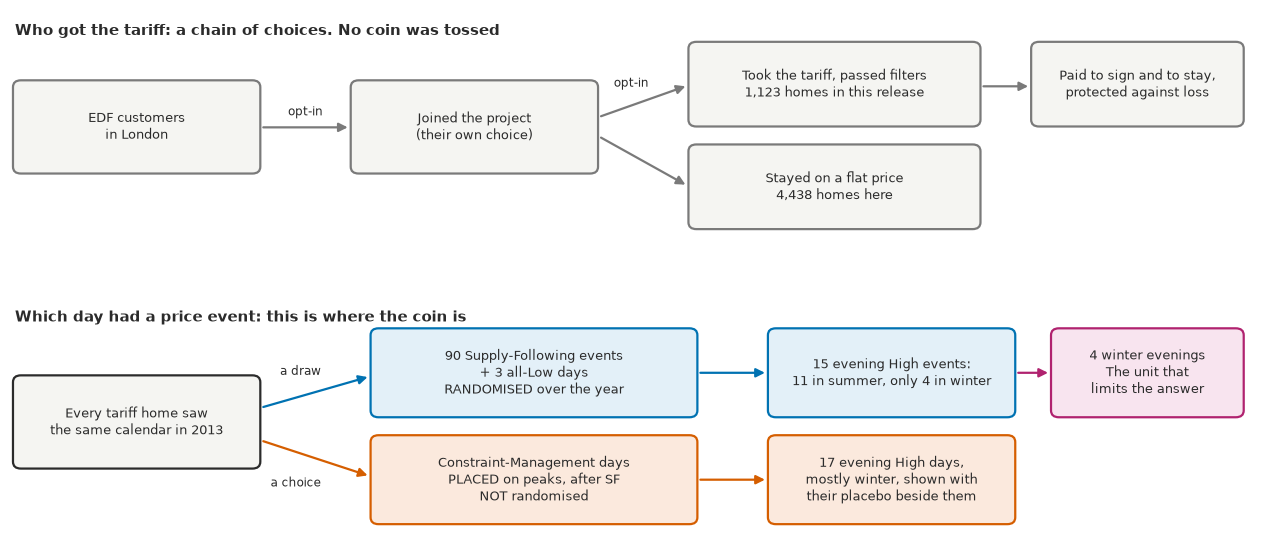
Read the top row as a warning and the bottom row as the opportunity. The guide to the trial says it plainly: the flat group "was not a true control". Only the blue line of the bottom row carries a causal claim, and the magenta box is what is left of it for the planner: 15 randomised evening High events, 11 in summer and only 4 in winter.
Here is the year itself: one column per day, one row per half-hour, on trial days that run from 05:00 to 05:00. Blue is randomised, orange is placed, and the dashed lines mark the evening.
calendar = store.load_json("calendar")
days_2013 = pd.date_range("2013-01-01", "2013-12-31", freq="D")
day_row = {d.strftime("%Y-%m-%d"): i for i, d in enumerate(days_2013)}
year = np.zeros((48, len(days_2013)), dtype=int)  # 0 default, 1-2 SF Low/High, 3-4 CM Low/High
OUT_DAYS = sorted(set(trial_day[hour_file["out_of_baseline"]]))
for e in calendar["events"]:
    if e["day"] in OUT_DAYS or e["day"] == "2013-03-29" or e["day"] not in day_row:
        continue
    start = pd.Timestamp(e["start_wall"])
    first = ((start.hour - 5) % 24) * 2 + start.minute // 30
    kind = (1 if e["band"] == "Low" else 2) + (0 if e["class"] == "single" else 2)
    year[first : first + e["slots"], day_row[e["day"]]] = kind
year[0:24, day_row["2013-03-29"]], year[24:36, day_row["2013-03-29"]], year[36:48, day_row["2013-03-29"]] = 3, 4, 3
for day in OUT_DAYS:
    if day in day_row:
        year[:, day_row[day]] = 5

colours = ["#f1f0ec", "#56b4e9", SF_C, "#e8963f", CM_C, "#7d7d7d"]
fig, ax = plt.subplots(figsize=(12.5, 4.6), layout="constrained")
ax.imshow(
    year,
    aspect="auto",
    interpolation="nearest",
    cmap=ListedColormap(colours),
    norm=BoundaryNorm(np.arange(-0.5, 6), 6),
    extent=(-0.5, 364.5, 29, 5),
)
ax.axhline(17, color=INK, lw=0.7, ls="--")
ax.axhline(23, color=INK, lw=0.7, ls="--")
sf_evening = cells[cells["effect"] == "SF High evening"]
winter = sf_evening[sf_evening["season"] == "gmt"]
for _, row in winter.iterrows():
    ax.annotate(
        pd.Timestamp(row["day"]).strftime("%-d %b"),
        (day_row[row["day"]], 17),
        xytext=(0, 18),
        textcoords="offset points",
        ha="center",
        fontsize=8.5,
        color=DUD_C if row["day"] == DUD_DAY else INK,
        weight="bold",
        arrowprops=dict(arrowstyle="-", color=DUD_C if row["day"] == DUD_DAY else INK, lw=0.9),
    )
months = pd.date_range("2013-01-01", "2013-12-01", freq="MS")
ax.set_xticks([day_row[m.strftime("%Y-%m-%d")] for m in months], [m.strftime("%b") for m in months])
ax.set_yticks([5, 11, 17, 23, 29], ["05:00", "11:00", "17:00", "23:00", "05:00"])
ax.set_ylabel("wall clock")
ax.legend(
    handles=[
        Patch(color=colours[2], label="SF High (randomised)"),
        Patch(color=colours[1], label="SF Low (randomised)"),
        Patch(color=colours[4], label="CM High (placed)"),
        Patch(color=colours[3], label="CM Low (placed)"),
        Patch(color=colours[5], label="days out of this analysis"),
    ],
    loc="lower center",
    ncols=5,
    bbox_to_anchor=(0.5, -0.27),
    fontsize=9,
)
ax.set_title(
    "2013 on one page. The four named evenings are all the randomised evidence for a winter peak",
    loc="left",
    fontsize=11,
);
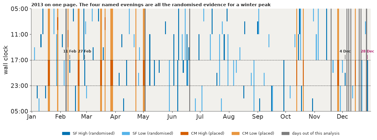
The SF blocks sweep the clock evenly, as a random calendar should, but most blue evening blocks fall between April and September, when evening load is low. The orange blocks cluster in the winter months a planner cares about, which is why they are tempting and why they must not be read as a coin toss.
Eight days differ between the price file and the published event table. We follow the table: 29 March behaves like a CM day and is kept as one, while 3 May and six days found only in the price file are left out of events and baseline alike. Those seven days and the three days priced Low all day are the grey columns.
2 · Failure 1: comparing the two groups
The obvious first analysis, M0, subtracts the flat homes' mean load from the tariff homes' during price events. The check is to run the same subtraction where no price could be acting: on evenings without an event, and in the months before and after the trial.
gap = 1000 * (fleet_kw - panel_kw)
evening = band == 2
event_days = np.unique(trial_day[effect >= 0])
quiet = evening & ~np.isin(trial_day, event_days) & usable


def m0_row(label, mask):
    return {"where": label, "tariff minus flat (W)": np.nanmean(gap[mask]), "hours": int(mask.sum())}


m0 = pd.DataFrame(
    [
        m0_row("SF High evening event", effect == EFFECTS.index("SF High evening")),
        m0_row("CM High evening event", effect == EFFECTS.index("CM High evening")),
        m0_row("2013 evenings on days with no event", quiet & in_2013),
        m0_row("Jul-Dec 2012 evenings, no price existed", quiet & pre_trial),
        m0_row("Jan-Feb 2014 evenings, prices over", quiet & after_trial),
    ]
).set_index("where")
print(m0.round(1).to_string())

weeks = pd.Series(gap[quiet], index=gmt[quiet]).resample("W").mean()
fig, ax = plt.subplots(figsize=(11.5, 4.5), layout="constrained")
ax.axvspan(pd.Timestamp("2013-01-01"), pd.Timestamp("2014-01-01"), color="#f1f0ec", lw=0, zorder=0)
ax.axhline(0, color=INK, lw=0.8)
ax.plot(weeks.index, weeks.to_numpy(), color=MUTED, lw=1.6, label="evenings with no event, weekly mean")
for name, colour, marker in (("SF High evening", SF_C, "o"), ("CM High evening", CM_C, "s")):
    sel = cells[cells["effect"] == name]
    y = [np.nanmean(gap[(effect == EFFECTS.index(name)) & (trial_day == d)]) for d in sel["day"]]
    ax.scatter(
        pd.to_datetime(sel["day"]), y, s=46, color=colour, marker=marker, edgecolor="w", lw=1, zorder=3, label=name
    )
ax.annotate("2013: the prices run", (pd.Timestamp("2013-02-10"), 48), fontsize=9.5, color=INK)
ax.set(ylabel="tariff minus flat homes (W)", ylim=(-165, 70))
ax.xaxis.set_major_formatter(mdates.ConciseDateFormatter(ax.xaxis.get_major_locator()))
ax.legend(loc="lower left", ncols=3, fontsize=9)
ax.set_title(
    "The two groups differ on evenings with no event, so their gap cannot be read as an effect", loc="left", fontsize=11
);
                                         tariff minus flat (W)  hours
where
SF High evening event                                    -68.7     72
CM High evening event                                    -84.7    102
2013 evenings on days with no event                      -36.4   1470
Jul-Dec 2012 evenings, no price existed                  -18.3   1104
Jan-Feb 2014 evenings, prices over                       -40.3    348
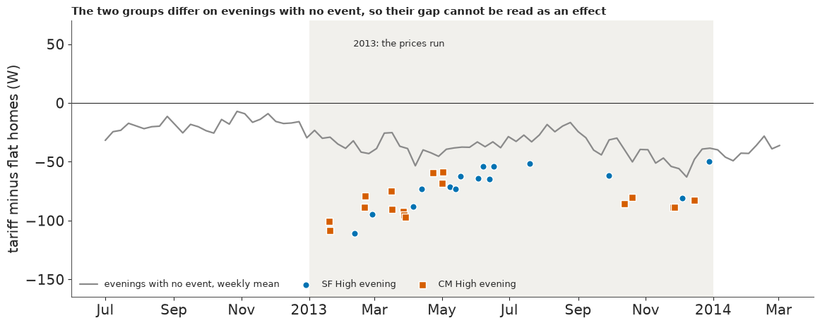
M0 says about -69 W on a randomised evening event. But the groups already sat 18 W apart in late 2012, before any price, 36 W apart on 2013 evenings with no event, and 40 W apart after the prices ended. People who chose differently differ anyway, and nothing here can say how much of the widening was behaviour and how much was who stayed. No kilowatt figure in this notebook comes from M0.
The fix is to stop comparing groups. Each tariff home becomes its own control, and the flat homes get one job: their mean load measures the weather, the football and every other shock all of London shares on the day. The price is that a habit kept all year would show no contrast between event days and ordinary days, so the within-home estimate misses any effect of simply being on the tariff. The planner's question is about events, so that is the right thing to measure.
3 · Failure 2: the clock
The price file is in wall-clock time. The meters are not: stamps exist at 01:00 on the day the clocks go forward, and none repeats in October. Nothing we found documents this release's convention, so the data have to tell us. The right convention puts the step in tariff homes' load where the price changes, in both seasons. Each bar is the mean step at one offset between meter stamp and price edge, across SF price edges, signed in the direction the price asks for.
clock = store.load_json("pilot_clock")
cost = store.load_json("clock_cost")
fig, axes = plt.subplots(1, 2, figsize=(11.5, 4.1), sharey=True, layout="constrained")
for ax, key, title, predicted in zip(axes, ("gmt_both", "bst_both"), ("GMT months", "BST months"), (1, -1)):
    t = clock["tables"][key]
    offset, mean, se = np.array(t["offset"]), np.array(t["mean_w"]), np.array(t["se_w"])
    ax.bar(
        offset,
        mean,
        yerr=1.96 * se,
        width=0.8,
        color=[SF_C if o == predicted else "#c7c7c7" for o in offset],
        error_kw=dict(lw=0.9, ecolor=INK),
    )
    ax.axvline(0, color=DUD_C, lw=1.4, ls="--")
    ax.annotate(
        "a naive join\nexpects it here",
        (0, 38),
        xytext=(-8, 0),
        textcoords="offset points",
        ha="right",
        fontsize=9,
        color=INK,
    )
    ax.axhline(0, color=INK, lw=0.7)
    ax.set_title(f"{title}, {t['n_events'][6]} edges", fontsize=10.5)
    ax.set(xticks=offset[::2])
    ax.tick_params(labelsize=10)
axes[0].set_ylabel("mean step, priced direction (W)", fontsize=10.5)
fig.supxlabel("offset in half-hours: stamp minus wall time of the price edge", fontsize=10.5)
fig.suptitle(
    "One rule fits both seasons: GMT all year, stamped at the end of the half-hour", x=0.01, ha="left", fontsize=11
)
naive, fixed = cost["wall_start"], cost["gmt_end"]
print("Mean tariff-minus-flat response inside SF runs, price direction (W). A timing check, never an effect:")
print(
    pd.DataFrame(
        {
            "naive join": [naive["gmt"]["mean_w"], naive["bst"]["mean_w"]],
            "gmt_end": [fixed["gmt"]["mean_w"], fixed["bst"]["mean_w"]],
        },
        index=["GMT", "BST"],
    )
    .assign(lost=lambda d: 1 - d["naive join"] / d["gmt_end"])
    .round(3)
    .to_string()
)
print(f"Clear of the worse neighbour by {clock['gate_margin_se']} se; the gate asked for 3");
Mean tariff-minus-flat response inside SF runs, price direction (W). A timing check, never an effect:
     naive join  gmt_end   lost
GMT      44.553   50.867  0.124
BST      28.419   32.089  0.114
Clear of the worse neighbour by 5.57 se; the gate asked for 3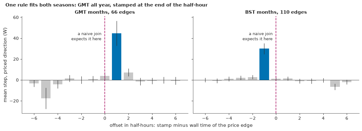
The step falls one slot after the edge in GMT months and one slot before it in BST months, clear of its neighbours by more than five standard errors. Only one convention predicts that pair: GMT all year, stamped at the end of each half-hour. A naive wall-clock join is 30 minutes out in both seasons, in opposite directions, and silently throws away about 12% of the response. The fix is one line in the data script: every hour here is two half-hours read in the meter's own frame.
4 · The fix: each home against itself
M1 is a plain descendant of the trial's published method. For home $h$ in hour $t$, in mean kW,
$$y_{ht} \sim \text{Normal}\Big(b_{h,s(t)} + \beta_h z_t + \sum_k \delta_{hk} X_{kt},\ \sigma_h^2\Big):$$
a home's usual load at this hour and day type ($s(t)$, 48 levels of wall hour x weekday or weekend), plus how much of today's shared shock it picks up ($z_t$, the flat homes' load against its usual level), plus 11 event effects $\delta_{hk}$: SF High and SF Low by time band, and three CM terms. Hours next to an event stay in the baseline, so M1 does not measure load moved into them; section 6 checks that once. The priors, in kW, are $b \sim N(0.4, 0.5)$, $\beta \sim N(1, 1)$, $\delta \sim N(0, 0.3)$. With $\sigma_h$ plugged in, each home's posterior is a small dense solve, so a fleet needs no sampler. What do the priors say about one hour?
prior_rng = np.random.default_rng(RANDOM_SEED + 1)
prior_load = prior_rng.normal(0.4, 0.5, 4000) + prior_rng.normal(1, 1, 4000) * prior_rng.normal(0, 0.1, 4000)
prior_delta = prior_rng.normal(0, 0.3, 4000)
prior_view = pd.DataFrame(
    {
        "5%": np.quantile(1000 * np.c_[prior_load, prior_delta], 0.05, axis=0),
        "median": np.median(1000 * np.c_[prior_load, prior_delta], axis=0),
        "95%": np.quantile(1000 * np.c_[prior_load, prior_delta], 0.95, axis=0),
    },
    index=["usual load at one hour (W)", "effect of an event (W)"],
)
print(prior_view.round(0).to_string())
print(f"Prior share of hours with a negative usual load: {(prior_load < 0).mean():.0%}")
print(
    f"Fleet mean load in 2013: {1000 * np.nanmean(fleet_kw[in_2013]):.0f} W, evening {1000 * np.nanmean(fleet_kw[in_2013 & evening]):.0f} W"
)
                               5%  median     95%
usual load at one hour (W) -465.0   400.0  1292.0
effect of an event (W)     -489.0     1.0   481.0
Prior share of hours with a negative usual load: 22%
Fleet mean load in 2013: 393 W, evening 554 W
Wide, on purpose: usual load from about -470 to 1,290 W, with 22% of draws impossibly negative, and event effects of up to about 500 W either way, against a real 2013 fleet mean of 393 W (554 W in the evening). With about 14,000 hours per home neither prior matters for the usual load. The one place a prior could bite is the home x event table, where a cell has a handful of hours per home, so there the data script uses a prior sd of 5 kW, to avoid shrinking event days towards zero and towards each other.
Now M1, live, on the 200 homes, with three baselines: the whole window from July 2012 to February 2014, 2013 alone, and 2013 with a term for each month x time band.
def deviation(keep):
    """z[t]: the flat homes' load in kW, against its own mean at that wall hour and day type."""
    z = np.zeros(n_hours)
    for s in range(48):
        at = level == s
        z[at] = panel_kw[at] - panel_kw[at & keep].mean()
    return np.nan_to_num(z)


def month_band(keep):
    """One indicator per month x time band, for the post-hoc local baseline."""
    key = pd.factorize(pd.Series(gmt.strftime("%Y-%m")).astype(str) + band.astype(str))[0]
    used, column = np.unique(key[keep], return_inverse=True)
    row = np.flatnonzero(keep)
    return sparse.csr_matrix((np.ones(row.size), (row, column)), shape=(n_hours, used.size))


def design(keep, local=False):
    """Hours x columns for M1: 48 levels, z, 11 effects, and month x band terms if asked."""
    rows = np.arange(n_hours)
    on = effect >= 0
    parts = [
        sparse.csr_matrix((np.ones(n_hours), (rows, level)), shape=(n_hours, 48)),
        sparse.csr_matrix(deviation(keep)[:, None]),
        sparse.csr_matrix((np.ones(on.sum()), (rows[on], effect[on])), shape=(n_hours, 11)),
    ]
    if local:
        parts.append(month_band(keep))
    return sparse.hstack(parts, format="csr")


def m1(kw, keep, local=False):
    """Closed-form fleet: conjugate Gaussian with plug-in sigma, home by home. Effects in W."""
    x_all = design(keep, local)
    q = x_all.shape[1] - 60
    prior_mean = np.r_[np.full(48, 0.4), 1.0, np.zeros(11 + q)]
    prior_prec = 1 / np.r_[np.full(48, 0.5), 1.0, np.full(11, 0.3), np.full(q, 0.5)] ** 2
    out = {
        "mean": np.full((len(kw), 11), np.nan),
        "sd": np.full((len(kw), 11), np.nan),
        "sigma": np.full(len(kw), np.nan),
        "kurtosis": np.full(len(kw), np.nan),
    }
    for h, y in enumerate(kw):
        ok = np.isfinite(y) & keep
        x, target = x_all[ok], y[ok]
        gram, moment = (x.T @ x).toarray(), x.T @ target
        variance = target.var()
        for _ in range(2):  # plug-in sigma: two passes are enough at these lengths
            precision = gram / variance + np.diag(prior_prec)
            theta = np.linalg.solve(precision, moment / variance + prior_prec * prior_mean)
            residual = target - x @ theta
            variance = float(np.mean(residual**2))
        cov = np.linalg.inv(gram / variance + np.diag(prior_prec))
        out["mean"][h] = 1000 * theta[49:60]
        out["sd"][h] = 1000 * np.sqrt(np.diag(cov)[49:60])
        out["sigma"][h] = 1000 * np.sqrt(variance)
        out["kurtosis"][h] = stats.kurtosis(residual)
    return out


meter_wh = meter_file["wh"].astype(float)
meter_wh[meter_file["wh"] == 65535] = np.nan
meters = meter_wh / 1000  # Wh in an hour is mean W, so this is mean kW
started = time.perf_counter()
with stage("M1, 200 homes, three baselines"):
    live = {
        "whole window": m1(meters, usable),
        "2013 only": m1(meters, usable & in_2013),
        "2013, month x band": m1(meters, usable & in_2013, local=True),
    }
pooled = store.load_json("pilot_placebo_benchmark")
names = {"whole window": "p6", "2013 only": "p6_2013only", "2013, month x band": "p6_local_2013only"}
compare = {}
for name, fit in live.items():
    for band_name in GATE_BANDS:
        k = EFFECTS.index(band_name)
        compare[(name, band_name)] = {
            "200 homes, live": fit["mean"][:, k].mean(),
            "se between homes": fit["mean"][:, k].std(ddof=1) / np.sqrt(len(meters)),
            "1,088 homes, stored": pooled[names[name]]["bands"][band_name]["mean_w"],
        }
print(f"Three fleets of {len(meters)} homes in {time.perf_counter() - started:.1f} s, no sampler")
print(pd.DataFrame(compare).T.round(1).to_string())
print(
    f"\nResiduals: excess kurtosis across homes, median {np.median(live['whole window']['kurtosis']):.1f} "
    f"(10-90%: {np.quantile(live['whole window']['kurtosis'], 0.1):.1f} to "
    f"{np.quantile(live['whole window']['kurtosis'], 0.9):.1f}); a Gaussian has 0"
)
Three fleets of 200 homes in 1.0 s, no sampler
                                    200 homes, live  se between homes  1,088 homes, stored
whole window       SF High evening            -45.0               5.9                -41.1
                   SF Low evening              38.6               7.8                 34.1
                   CM High evening            -60.0               8.9                -48.4
2013 only          SF High evening            -32.8               5.2                -31.6
                   SF Low evening              50.6               7.9                 43.7
                   CM High evening            -47.4               8.0                -39.5
2013, month x band SF High evening            -32.1               5.1                -29.4
                   SF Low evening              51.4               7.7                 42.7
                   CM High evening            -54.1               9.1                -44.2

Residuals: excess kurtosis across homes, median 11.5 (10-90%: 4.1 to 30.1); a Gaussian has 0
Three fleets in a second. The 200 homes land within about 1.3 standard errors (5-9 W) of the 1,088-home fleet in every cell, so they are a check, not the estimate. The residuals are far from Gaussian, with a median excess kurtosis near 12. A mean does not need Gaussian noise to be unbiased, but one home's posterior sd is too small, so standard errors from here on come from the spread between homes and between events.
Three checks before any delivery number
First, is the calendar really random? The seed and rule were never published, so the test is approximate: flat homes never saw a price, so their evening load on SF days should look like any other day's, net of month and day type. We shuffled the SF days 20,000 times under a weekly limit.
balance = store.load_json("pilot_balance")
rows = {
    name: balance["sf_all"][key]
    for name, key in (("All 90 SF days", "all"), ("GMT months", "gmt"), ("BST months", "bst"))
}
rows["The 15 evening High days (not gated)"] = balance["sf_evening_high"]["all"]
print(
    pd.DataFrame(rows)
    .T[["obs_w", "null_sd", "z"]]
    .rename(columns={"obs_w": "SF minus default (W)", "null_sd": "null sd (W)"})
    .round(2)
    .to_string()
)
                                      SF minus default (W)  null sd (W)     z
All 90 SF days                                       -2.04         4.10 -0.49
GMT months                                           -7.22         7.09 -0.98
BST months                                            1.30         4.98  0.23
The 15 evening High days (not gated)                 10.25         8.87  1.18
It passes. Flat homes' load on the 90 SF days is 2 W below other days (z about -0.5), neither season stands out, and the 15 evening High days sit about one null sd above. The test has no weather data and the weekly limit barely binds, so it is weak, but it gives no reason to doubt the randomisation.
Second, a placebo: move the 2013 calendar back 364 days, into late 2012 when no price existed, and run the same fit. If the baseline is honest, every cell should read within about 10 W of zero, with a standard error under 5 W; a bias of 25 W would sink the estimate altogether.
placebo = pooled["p5"]["bands"]
no_dud = pooled["p5_no28dec"]["bands"]
placebo_view = pd.DataFrame(
    {
        b: {
            "events": placebo[b]["events"],
            "mean (W)": placebo[b]["mean_w"],
            "se homes": placebo[b]["se_home_w"],
            "se events": placebo[b]["se_event_w"],
            "without the shifted 28 Dec": no_dud[b]["mean_w"],
        }
        for b in GATE_BANDS
    }
).T
print(
    "Placebo: the 2013 calendar moved back 364 days, Jul-Dec 2012, no prices existed. Gate: |mean| <= 10 W, se <= 5 W"
)
print(placebo_view.round(1).to_string())
print(
    f"Homes: {pooled['p5']['homes']}. Passes: {pooled['p5_passes']}. Over the 25 W line that ends the estimate: {pooled['p5_over25']}"
)
shifted = next(c for c in pooled["p5"]["cells"] if c["day"] == DUD_DAY and c["effect"] == "SF High evening")
dud_column = placebo_cells.index[(placebo_cells["day"] == DUD_DAY) & (placebo_cells["effect"] == "SF High evening")][0]
dud_se = np.nanstd(placebo_table[:, dud_column], ddof=1) / np.sqrt(np.isfinite(placebo_table[:, dud_column]).sum())
print(
    f"The placebo cell for 29 Dec 2012 alone, the day that lines up with 28 Dec 2013: {shifted['w']:+.1f} W (se {dud_se:.1f}), no price at all"
)
print(
    "All four SF High placebo cells:",
    [f"{c['w']:+.1f} W" for c in pooled["p5"]["cells"] if c["effect"] == "SF High evening"],
)
print(
    f"Post-hoc, not a rescue: with month x band terms CM's placebo is {pooled['p5_local']['bands']['CM High evening']['mean_w']:+.1f} W, "
    f"SF High evening {pooled['p5_local']['bands']['SF High evening']['mean_w']:+.1f} W"
)
Placebo: the 2013 calendar moved back 364 days, Jul-Dec 2012, no prices existed. Gate: |mean| <= 10 W, se <= 5 W
                 events  mean (W)  se homes  se events  without the shifted 28 Dec
SF High evening     4.0      -6.1       4.4       10.6                         1.1
SF Low evening     10.0      -0.2       3.1        2.7                        -0.2
CM High evening     5.0      13.2       4.2        2.1                        12.9
Homes: 963. Passes: False. Over the 25 W line that ends the estimate: False
The placebo cell for 29 Dec 2012 alone, the day that lines up with 28 Dec 2013: -27.7 W (se 12.5), no price at all
All four SF High placebo cells: ['+2.0 W', '+10.5 W', '-4.4 W', '-27.7 W']
Post-hoc, not a rescue: with month x band terms CM's placebo is +4.9 W, SF High evening -6.4 W
This is failure 3. SF Low passes (-0.2 W). SF High has a small mean, -6 W, but a standard error of 11 W from four evenings, twice the limit. And the placed peak days read +13 W with no price at all. Nothing comes near 25 W, so the estimate survives in a reduced form: only the randomised SF evenings carry a delivery estimate, and CM days stay on the page, labelled, outside every range. Month x band terms bring CM's placebo down to about +5 W, which hints that one shared-shock coefficient misses the winter evening rise, but that was tried after seeing the failure and does not undo it.
One cell deserves a note. The 2012 evening that lines up with 28 December reads about -28 W (se 12) with no price at all, while the other three SF High placebo cells are small. One cell at 2.2 se does not make Christmas week noisy (section 6 finds it about as quiet as any other), but it does warn us against reading a near-zero response on 28 December 2013 as proof that something went wrong.
Third, a benchmark: does the fleet reproduce the published ranges, -70 to -30 W on peak days and -50 to -15 W on SF evenings? We run it on five baselines.
baselines = {
    "Whole window (the plan)": "p6",
    "Same, without 28 Dec": "p6_no28dec",
    "2013 only": "p6_2013only",
    "2013, month x band (post-hoc)": "p6_local_2013only",
    "Same, without 28 Dec ": "p6_local_2013_no28dec",
}
window = pd.DataFrame({k: {b: pooled[v]["bands"][b]["mean_w"] for b in GATE_BANDS} for k, v in baselines.items()}).T
print(
    f"Benchmark on {pooled['p6']['homes']:,} homes (gate: CM -70 to -30 W, SF -50 to -15 W). Passes: {pooled['p6_passes']}"
)
print(window.round(1).to_string())

sf_high = cells[cells["effect"] == "SF High evening"]
event_hours_w = sf_high["hours"].to_numpy(float)
picks = np.random.default_rng(RANDOM_SEED + 5).integers(0, len(sf_high), (20_000, len(sf_high)))
print("\nSF High evening, hour-weighted, resampling the 15 events (the calendar's sample, not the homes'):")
for name, key in (("2013, month x band", "local"), ("whole window", "plan")):
    event_w = np.nanmean(home_tables[key][:, sf_high.index], axis=0)
    resampled = (event_w[picks] * event_hours_w[picks]).sum(axis=1) / event_hours_w[picks].sum(axis=1)
    print(
        f"  {name}: {np.average(event_w, weights=event_hours_w):.1f} W, 90% interval "
        f"{np.quantile(resampled, 0.05):.1f} to {np.quantile(resampled, 0.95):.1f} W"
    )

fig, axes = plt.subplots(1, 2, figsize=(12.5, 4.5), width_ratios=(1, 1.35), layout="constrained")
ax = axes[0]
ax.axhspan(-10, 10, color="#f1f0ec", lw=0, label="gate: within 10 W")
for line in (-25, 25):
    ax.axhline(line, color=DUD_C, lw=1, ls="--")
ax.annotate(
    "past 25 W the estimate is abandoned",
    (2.42, 25),
    xytext=(0, 3),
    textcoords="offset points",
    ha="right",
    fontsize=8.5,
    color=INK,
)
for i, b in enumerate(GATE_BANDS):
    colour = CM_C if b.startswith("CM") else SF_C
    r = placebo[b]
    ax.errorbar(
        i, r["mean_w"], 1.96 * max(r["se_home_w"], r["se_event_w"]), fmt="o", ms=9, color=colour, capsize=0, lw=1.8
    )
    ax.annotate(
        f"{r['mean_w']:+.1f} W", (i, r["mean_w"]), xytext=(10, 2), textcoords="offset points", fontsize=9, color=INK
    )
ax.axhline(0, color=INK, lw=0.7)
ax.set_xticks(range(3), ["SF High\n4 events", "SF Low\n10 events", "CM High\n5 events"])
ax.set(xlim=(-0.45, 2.45), ylim=(-40, 40), ylabel="W, with no price in existence", title="Before prices: the placebo")
ax = axes[1]
y = np.arange(len(window))[::-1]
for b, colour, marker in zip(GATE_BANDS, (SF_C, SKY, CM_C), ("o", "D", "s")):
    ax.scatter(window[b], y, s=70, color=colour, marker=marker, edgecolor="w", lw=1, zorder=3, label=b)
ax.axvline(0, color=INK, lw=0.7)
ax.set_yticks(y, [k.strip() for k in window.index])
ax.set(xlabel="effect of the event (W)", title="During prices: the same fleet, five baselines")
ax.legend(loc="center", fontsize=9, bbox_to_anchor=(0.72, 0.55));
Benchmark on 1,088 homes (gate: CM -70 to -30 W, SF -50 to -15 W). Passes: True
                               SF High evening  SF Low evening  CM High evening
Whole window (the plan)                  -41.1            34.1            -48.4
Same, without 28 Dec                     -43.9            34.1            -48.3
2013 only                                -31.6            43.7            -39.5
2013, month x band (post-hoc)            -29.4            42.7            -44.2
Same, without 28 Dec                     -31.8            42.7            -44.2

SF High evening, hour-weighted, resampling the 15 events (the calendar's sample, not the homes'):
  2013, month x band: -29.2 W, 90% interval -36.3 to -22.7 W
  whole window: -41.6 W, 90% interval -47.3 to -35.4 W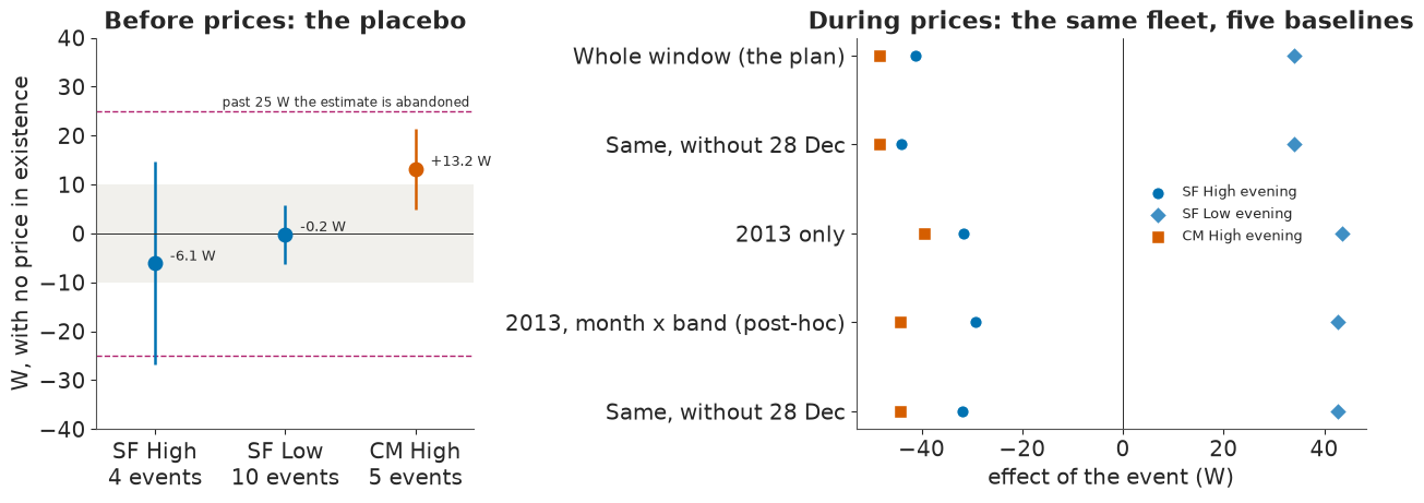
It passes on every baseline, but the window moves everything. With the pre-trial months in, every evening effect is about 10 W more negative, for High and Low prices alike (SF High -41 against -29 W, SF Low +34 against +43 W). A real response would not push a Low price the same way, so this looks like the 2013 level shift that widened the group gap in section 2. On SF High evenings it is about 15 W in summer and only 3 W in winter.
The quantity we want compares event days with ordinary days of the trial, which favours the 2013 baseline with month x band terms. We only made that argument after seeing the placebo, though, so the whole-window baseline, the one we started with, stays as the other end of a range. Taken from the home x event table, where CM hours are out of every SF figure: a randomised SF evening High event cut about 29-42 W per home, out of an evening load near 550 W, as a mean over the priced hours. Resampling the 15 events gives a 90% interval of about -36 to -23 W around one end and -47 to -35 W around the other.
The placebo could not test the two February evenings that carry most of the winter signal, because there is no February 2012. The last cell moves them forward to February 2014, after the prices ended.
def fleet_fit(keep):
    """The fleet's mean load against M1's baseline, fitted to default hours inside `keep`, in W."""
    default_hours = keep & usable & (effect < 0)
    levels_x = sparse.csr_matrix((np.ones(n_hours), (np.arange(n_hours), level)), shape=(n_hours, 48))
    fleet_x = sparse.hstack(
        [levels_x, sparse.csr_matrix(deviation(keep & usable)[:, None]), month_band(keep)], format="csr"
    )
    solution = sparse.linalg.lsqr(fleet_x[default_hours], fleet_kw[default_hours], atol=1e-9, btol=1e-9, iter_lim=4000)[0]
    return 1000 * (fleet_kw - fleet_x @ solution)


whole_response = fleet_fit(np.ones(n_hours, dtype=bool))
forward = {}
for day in ("2013-02-11", "2013-02-27"):
    event = sf_high[sf_high["day"] == day].iloc[0]
    moved_day = (pd.Timestamp(day) + pd.Timedelta(days=364)).strftime("%Y-%m-%d")
    moved_hours = (
        (trial_day == moved_day) & (hour_of_day >= event["start_hour"]) & (hour_of_day < event["start_hour"] + event["event_hours"])
    )
    forward[f"{day} moved to {moved_day}"] = np.nanmean(whole_response[moved_hours])
late_quiet = quiet & after_trial
print("The February evenings moved forward 364 days, prices over, fleet mean, W:", {k: round(v, 1) for k, v in forward.items()})
print(
    "Spread of a Jan-Feb 2014 default evening, same fit:",
    f"{pd.Series(whole_response[late_quiet]).groupby(trial_day[late_quiet]).mean().std():.1f} W",
)
The February evenings moved forward 364 days, prices over, fleet mean, W: {'2013-02-11 moved to 2014-02-10': np.float64(17.9), '2013-02-27 moved to 2014-02-26': np.float64(11.7)}
Spread of a Jan-Feb 2014 default evening, same fit: 9.4 W
Both read on the side of no response, +18 and +12 W, within two sd (9 W) of an ordinary 2014 evening. No sign of a false cut there, on a check added after the fact.
5 · Failure 4: the robust model
Residuals with an excess kurtosis near 12 are the textbook case for a Student-t likelihood. M2 keeps M1's structure and changes one line:
$$y_{ht} \sim \text{StudentT}\big(\nu_h,\ b_{h,s(t)} + \beta_h z_t + \sum_k \delta_{hk} X_{kt},\ \sigma_h\big), \qquad \nu_h = 2 + \text{Gamma}(2, 0.1).$$
The floor of 2 keeps the variance finite, and the prior puts $\nu$ near 20, so the data must argue for
heavy tails. We fit every tenth home of the 200 with one compiled nutpie model and with_data, and
compare with a stored 100-home run.
with pm.Model() as m2:
    y_data = pm.Data("y", np.zeros(200))
    x_data = pm.Data("X", np.zeros((200, 11)))
    z_data = pm.Data("z", np.zeros(200))
    s_data = pm.Data("s", np.zeros(200, dtype="int64"))
    b = pm.Normal("b", 0.4, 0.5, shape=48)
    beta = pm.Normal("beta", 1, 1)
    delta = pm.Normal("delta", 0, 0.3, shape=11)
    sigma = pm.LogNormal("sigma", np.log(0.3), 0.7)
    nu_extra = pm.Gamma("nu_extra", 2, 0.1)
    location = b[s_data] + beta * z_data + x_data @ delta
    pm.StudentT("obs", nu=2 + nu_extra, mu=location, sigma=sigma, observed=y_data, shape=location.shape)

with stage("M2, compile"):
    compiled = nutpie.compile_pymc_model(m2)

z_all = deviation(usable)
effect_hours = np.zeros((n_hours, 11))
effect_hours[np.flatnonzero(effect >= 0), effect[effect >= 0]] = 1.0
student_rows = []
with stage("M2, 20 homes"):
    for i, h in enumerate(range(0, len(meters), 10)):
        ok = np.isfinite(meters[h]) & usable
        started = time.perf_counter()
        trace = nutpie.sample(
            compiled.with_data(y=meters[h, ok], X=effect_hours[ok], z=z_all[ok], s=level[ok].astype("int64")),
            chains=4,
            tune=500,
            draws=500,
            cores=CHAINS_AT_ONCE,
            seed=RANDOM_SEED + i,
            progress_bar=False,
            save_warmup=False,
            store_mass_matrix=False,
            store_gradient=False,
            store_unconstrained=False,
        )
        post = trace.posterior.to_dataset()
        hat = az.rhat(post)
        hat = hat.to_dataset() if hasattr(hat, "to_dataset") else hat
        ess = az.ess(post)
        ess = ess.to_dataset() if hasattr(ess, "to_dataset") else ess
        student_rows.append(
            {
                "home": int(meter_file["homes"][h]),
                "row": h,
                "seconds": time.perf_counter() - started,
                "max r_hat": max(float(np.nanmax(hat[v].values)) for v in hat.data_vars),
                "min ESS": min(float(np.nanmin(ess[v].values)) for v in ess.data_vars),
                "divergences": int(trace.sample_stats["diverging"].values.sum()),
                "nu": 2 + float(post["nu_extra"].median()),
                **{
                    b_name: 1000 * float(post["delta"].mean(("chain", "draw")).values[EFFECTS.index(b_name)])
                    for b_name in GATE_BANDS
                },
            }
        )
student = pd.DataFrame(student_rows)
print(
    student[["seconds", "max r_hat", "min ESS", "divergences", "nu"]]
    .describe()
    .loc[["min", "50%", "max"]]
    .round(3)
    .to_string()
)
print(
    f"Homes at max r_hat <= 1.01: {(student['max r_hat'] <= 1.01).sum()} of {len(student)}; <= 1.02: {(student['max r_hat'] <= 1.02).sum()}"
)
print(
    "Worst of the 20:",
    student.sort_values("max r_hat")
    .iloc[-1][["home", "max r_hat", "min ESS", "divergences", "seconds"]]
    .round(2)
    .to_dict(),
)
paired = {
    b_name: live["whole window"]["mean"][student["row"].to_numpy(), EFFECTS.index(b_name)]
    - student[b_name].to_numpy()
    for b_name in GATE_BANDS
}
print(
    pd.DataFrame(
        {
            b_name: {
                "M1 mean of 20 homes (W)": live["whole window"]["mean"][
                    student["row"].to_numpy(), EFFECTS.index(b_name)
                ].mean(),
                "M2 mean of 20 homes (W)": student[b_name].mean(),
                "paired se (W)": paired[b_name].std(ddof=1) / np.sqrt(len(student)),
            }
            for b_name in GATE_BANDS
        }
    )
    .round(1)
    .to_string()
)

fit_pilot, location_pilot = store.load_json("pilot_fit"), store.load_json("pilot_mean_location")
print(
    f"\nStored, 100 homes: median {fit_pilot['median_s']:.1f} s a fit, {fit_pilot['total_div']} divergences, "
    f"{fit_pilot['rhat_le_1.01']} homes at r_hat <= 1.01 and {fit_pilot['rhat_le_1.02']} at 1.02, "
    f"median nu {fit_pilot['nu_median']:.3f}. Worst homes:"
)
print(pd.DataFrame(fit_pilot["worst"])[["home", "rhat", "nu", "div"]].head(3).to_string(index=False))
     seconds  max r_hat   min ESS  divergences     nu
min    4.566      1.007     6.157          0.0  2.001
50%    5.210      1.011  2855.401          0.0  2.003
max   24.476      1.734  3434.193          0.0  2.365
Homes at max r_hat <= 1.01: 9 of 20; <= 1.02: 18
Worst of the 20: {'home': 1704.0, 'max r_hat': 1.73, 'min ESS': 6.16, 'divergences': 0.0, 'seconds': 5.15}
                         SF High evening  SF Low evening  CM High evening
M1 mean of 20 homes (W)            -62.3            49.9            -85.9
M2 mean of 20 homes (W)            -39.1            -4.4            -26.2
paired se (W)                        7.3            18.3             15.0

Stored, 100 homes: median 10.1 s a fit, 0 divergences, 40 homes at r_hat <= 1.01 and 97 at 1.02, median nu 2.005. Worst homes:
 home   rhat  nu  div
 1704 1.7357 2.0    0
 3047 1.7326 2.0    0
 4687 1.5277 2.0    0
Two things have gone wrong, and the sampler reports neither as a failure.
First, nu sits on its floor: median 2.003, highest 2.37, as in the 100 stored fits. Hourly load is
more heavy-tailed than even this model allows. Second, mixing: no divergences at all, yet only 9 of 20
homes reach r_hat 1.01 (40 of the stored 100). Most misses are just too few draws and clear at 2,000
draws, but in three homes (1704, 3047, 4687) the chains sit in different modes of b or sigma and
longer runs did not cure it. Home 1704 is here, at r_hat 1.73 with a minimum ESS of 6 and still no
divergence. We did not establish why.
The serious problem is the answer. M2's effects are smaller than M1's in all three bands, and on SF Low it is not even clearly positive (+50 W against -4 W, paired se 18). Where does an event take its watts from? Compare the 200 homes' hours during evening events with the same homes, hours and day types on nearby default days, one quantile at a time.
QUANTILES = np.arange(0.05, 0.96, 0.05)


def shift_gaps(hours_on):
    """These hours minus matched default hours within 28 days, by quantile of each home's own hours, W."""
    clean = (effect < 0) & usable & in_2013
    matched = []
    for t in hours_on:
        window_hours = np.arange(max(t - 672, 0), min(t + 672, n_hours))
        matched.append(window_hours[clean[window_hours] & (level[window_hours] == level[t])])
    matched = np.concatenate(matched)
    usual = np.nanquantile(meters[:, matched], QUANTILES, axis=1)
    gaps = np.nanquantile(meters[:, hours_on], QUANTILES, axis=1) - usual
    mean_gap = np.nanmean(meters[:, hours_on], axis=1) - np.nanmean(meters[:, matched], axis=1)
    return 1000 * gaps, 1000 * usual, 1000 * mean_gap, 1000 * np.nanmean(meters[:, matched], axis=1)


def shift_function(which):
    """The shift across 200 homes: mean gap by quantile, its se, the mean hour, and the gap in percent."""
    gaps, usual, mean_gap, mean_usual = shift_gaps(np.flatnonzero((effect == EFFECTS.index(which)) & in_2013))
    return (
        gaps.mean(axis=1),
        gaps.std(axis=1, ddof=1) / np.sqrt(len(meters)),
        mean_gap.mean(),
        100 * gaps.mean(axis=1) / usual.mean(axis=1),
        100 * mean_gap.mean() / mean_usual.mean(),
    )


def no_price_shifts(which, draws=40):
    """The same recipe on calendars with no price: each event moved whole weeks onto default hours."""
    hours_on = np.flatnonzero((effect == EFFECTS.index(which)) & in_2013)
    clean = (effect < 0) & usable & in_2013
    move_rng = np.random.default_rng(RANDOM_SEED + 4)
    options = []
    for day in np.unique(trial_day[hours_on]):
        block = hours_on[trial_day[hours_on] == day]
        moves = [block + 168 * w for w in range(-6, 7) if w and (block + 168 * w).max() < n_hours]
        options.append([m for m in moves if clean[m].all()])
    return np.array(
        [
            shift_gaps(np.concatenate([o[move_rng.integers(len(o))] for o in options]))[0].mean(axis=1)
            for _ in range(draws)
        ]
    )


q = QUANTILES
shift_sf, shift_se, shift_mean, percent_sf, percent_mean = shift_function("SF High evening")
shift_cm, shift_cm_se, cm_mean, percent_cm, _ = shift_function("CM High evening")
control_sf, control_cm = no_price_shifts("SF High evening"), no_price_shifts("CM High evening")
print(
    pd.DataFrame(
        {
            "SF High evening (W)": shift_sf,
            "no-price calendars, mean (W)": control_sf.mean(axis=0),
            "SF minus no-price (W)": shift_sf - control_sf.mean(axis=0),
            "SF, percent of that quantile": percent_sf,
            "CM High evening (W)": shift_cm,
            "CM no-price calendars, mean (W)": control_cm.mean(axis=0),
        },
        index=[f"{p:.0%}" for p in q],
    )
    .T.round(1)
    .iloc[:, [1, 5, 9, 13, 15, 16, 17, 18]]
    .to_string()
)
print(f"Mean hour: SF {shift_mean:.0f} W ({percent_mean:.1f}%), CM {cm_mean:.0f} W")
print(
    f"No-price calendars at the 95th percentile, 5-95%: {np.quantile(control_sf[:, -1], 0.05):.0f} to "
    f"{np.quantile(control_sf[:, -1], 0.95):.0f} W; at the median {np.quantile(control_sf[:, 9], 0.05):.0f} to "
    f"{np.quantile(control_sf[:, 9], 0.95):.0f} W"
)

fig, axes = plt.subplots(1, 2, figsize=(12.5, 4.6), width_ratios=(1.2, 1), layout="constrained")
ax = axes[0]
for values, se, colour, label, marker in (
    (shift_sf, shift_se, SF_C, "SF High evening", "o"),
    (shift_cm, shift_cm_se, CM_C, "CM High evening (not randomised)", "s"),
):
    ax.fill_between(q * 100, values - 1.96 * se, values + 1.96 * se, color=colour, alpha=0.14, lw=0)
    ax.plot(q * 100, values, color=colour, lw=2, marker=marker, ms=5, label=label)
ax.plot(q * 100, control_sf.mean(axis=0), color=MUTED, lw=1.8, ls="--", label="SF recipe on no-price calendars")
ax.axhline(0, color=INK, lw=0.8)
ax.axvspan(40, 60, color="#f1f0ec", lw=0, zorder=0)
ax.annotate("a robust fit\nlooks here", (50, -165), ha="center", fontsize=9.5, color=INK)
ax.annotate("the busiest\nhours", (86, -175), ha="center", fontsize=9.5, color=INK)
ax.set(
    xlabel="quantile of a home's hours, from quiet to busy",
    ylabel="event minus matched default hours (W)",
    ylim=(-200, 40),
)
ax.legend(loc="lower left", fontsize=9)
ax.set_title("The top quantiles move most, and part of that shift appears with no price", loc="left", fontsize=11)

ax = axes[1]
order = list(GATE_BANDS)
y = np.arange(3)[::-1]
for yi, b_name in zip(y, order):
    r = location_pilot["bands"][b_name]
    ax.plot([r["m1"], r["m2"]], [yi, yi], color="#c7c7c7", lw=3, zorder=1)
    ax.scatter(r["m1"], yi, s=95, color=SF_C, zorder=3, label="M1, the mean" if yi == 2 else None)
    ax.scatter(
        r["m2"],
        yi,
        s=95,
        facecolor="w",
        edgecolor=DUD_C,
        lw=2,
        zorder=3,
        label="M2, Student-t location" if yi == 2 else None,
    )
    ax.scatter(r["gd"], yi, s=80, marker="x", color=INK, zorder=4, label="group difference, a rough check" if yi == 2 else None)
ax.axvline(0, color=INK, lw=0.7)
ax.set_yticks(y, ["SF High\nevening", "SF Low\nevening", "CM High\nevening"])
ax.set(xlabel="what each method reads, same 100 homes (W)", ylim=(-0.6, 2.9))
ax.legend(loc="upper center", ncols=3, fontsize=8.2, bbox_to_anchor=(0.5, 1.0), handletextpad=0.1, columnspacing=0.7)
ax.set_title("The robust fit misses SF Low and CM. On SF High the gap is not clear", loc="left", fontsize=11);
                                  10%   30%   50%   70%   80%   85%   90%    95%
SF High evening (W)               2.3  -5.7 -15.2 -14.4 -27.4 -59.9 -65.9 -135.8
no-price calendars, mean (W)      6.1   4.1   5.9   5.3   4.9  -0.6 -14.6  -36.6
SF minus no-price (W)            -3.8  -9.9 -21.1 -19.7 -32.3 -59.3 -51.3  -99.1
SF, percent of that quantile      1.2  -1.8  -3.5  -2.4  -3.7  -6.9  -6.4  -10.4
CM High evening (W)               5.4  -1.8  -8.2 -45.8 -48.0 -50.8 -85.4 -137.2
CM no-price calendars, mean (W)  18.4  22.1  19.5  18.1  19.8  21.5  16.8   -3.1
Mean hour: SF -23 W (-4.3%), CM -27 W
No-price calendars at the 95th percentile, 5-95%: -107 to 11 W; at the median -17 to 24 W
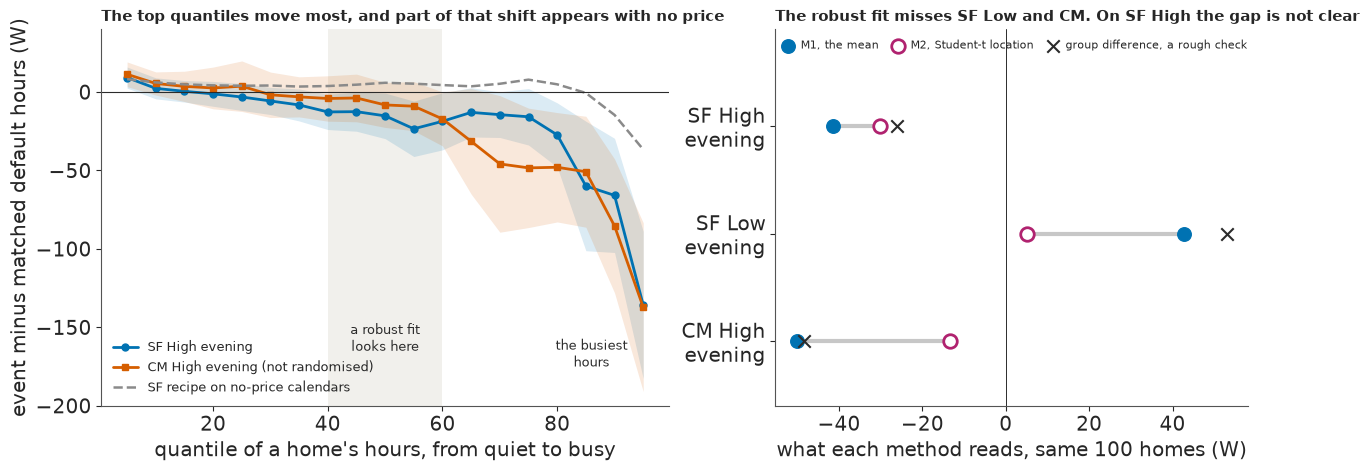
On SF evenings the median hour reads about 15 W lower and the 95th percentile about 136 W lower. Part of that is an artefact: quantiles of 72 hours compared with those of many more are biased even without a price, and the same events moved onto default weeks (the dashed line) read about +6 W at the median and -37 W at the 95th. Net of that, the median moves about 21 W and the 95th about 99 W. As a share of each quantile the shift is -3.5% at the median and -10% at the 95th, against -4% for the mean hour, so busy hours lose most watts partly because they are bigger. Moved or skipped cooking and washing is the likely reading, though the data have no appliance column.
The right panel is the lesson. A Student-t location follows the typical hour and discounts busy hours as outliers; it is not a mean. On the 100 stored homes it sees about a quarter of the peak-day cut and an eighth of the SF Low rise; it differs from the mean by more than 20% in all three bands. On the randomised High band the gap is less clear (-30 against -41 W, about 1.7 paired se, inside the baseline range), so M2 is clearly wrong for SF Low and the peak days and only possibly wrong for SF High.
The fix is to ask what adds up at a substation: the sum of the homes' means. A likelihood that tracks the typical hour understates the change wherever busy hours carry it, so M1 carries every kW figure, on that argument rather than because M2 was shown wrong on the headline band.
6 · Every evening counts
Here are the 15 randomised evening events, one panel each, as the whole fleet's response hour by hour against a baseline fitted to the default hours of 2013.
with stage("Fleet curves"):
    clean_hours = usable & in_2013 & (effect < 0)
    fleet_response = fleet_fit(in_2013)
print(f"Default-hour fit: residual sd {np.nanstd(fleet_response[clean_hours]):.1f} W per hour")

evening_events = cells[cells["effect"] == "SF High evening"].sort_values("day")
local_means = pd.Series(
    np.nanmean(home_tables["local"][:, evening_events.index], axis=0), index=evening_events["day"]
)
fig, axes = plt.subplots(3, 5, figsize=(13, 6.6), sharex=True, sharey=True, layout="constrained")
for ax, (_, event) in zip(axes.flat, evening_events.iterrows()):
    on_day = trial_day == event["day"]
    t = hour_of_day[on_day] + np.where(hour_of_day[on_day] < 5, 24, 0)
    order = np.argsort(t)
    show = (t[order] >= 12) & (t[order] <= 26)
    start, stop = event["start_hour"], event["start_hour"] + event["event_hours"]
    colour = DUD_C if event["day"] == DUD_DAY else SF_C
    is_winter = event["season"] == "gmt"
    ax.set_facecolor("#eef4f9" if is_winter else "#ffffff")
    ax.axvspan(max(start, 12), min(stop, 26), color=colour, alpha=0.16, lw=0)
    ax.axvspan(17, 23, ymin=0, ymax=0.03, color=INK, lw=0)
    ax.axhline(0, color=INK, lw=0.6)
    ax.plot(t[order][show], fleet_response[on_day][order][show], color=colour, lw=1.9)
    ax.text(
        0.03,
        0.91,
        f"{pd.Timestamp(event['day']):%-d %b}",
        transform=ax.transAxes,
        fontsize=9.5,
        weight="bold",
        color=INK,
    )
    ax.text(
        0.97, 0.91, f"{local_means[event['day']]:+.0f} W", transform=ax.transAxes, ha="right", fontsize=9.5, color=INK
    )
axes[0, 0].set(ylim=(-140, 140), xlim=(12, 26), xticks=[12, 17, 23], xticklabels=["12:00", "17:00", "23:00"])
for ax in axes[:, 0]:
    ax.set_ylabel("fleet response (W)")
fig.suptitle(
    "15 randomised evenings in date order. Shaded: the High price. Tinted panels: winter. Black bar: 17:00-23:00. Corner figure: event hours within it",
    x=0.01,
    ha="left",
    fontsize=11,
);
Default-hour fit: residual sd 12.4 W per hour
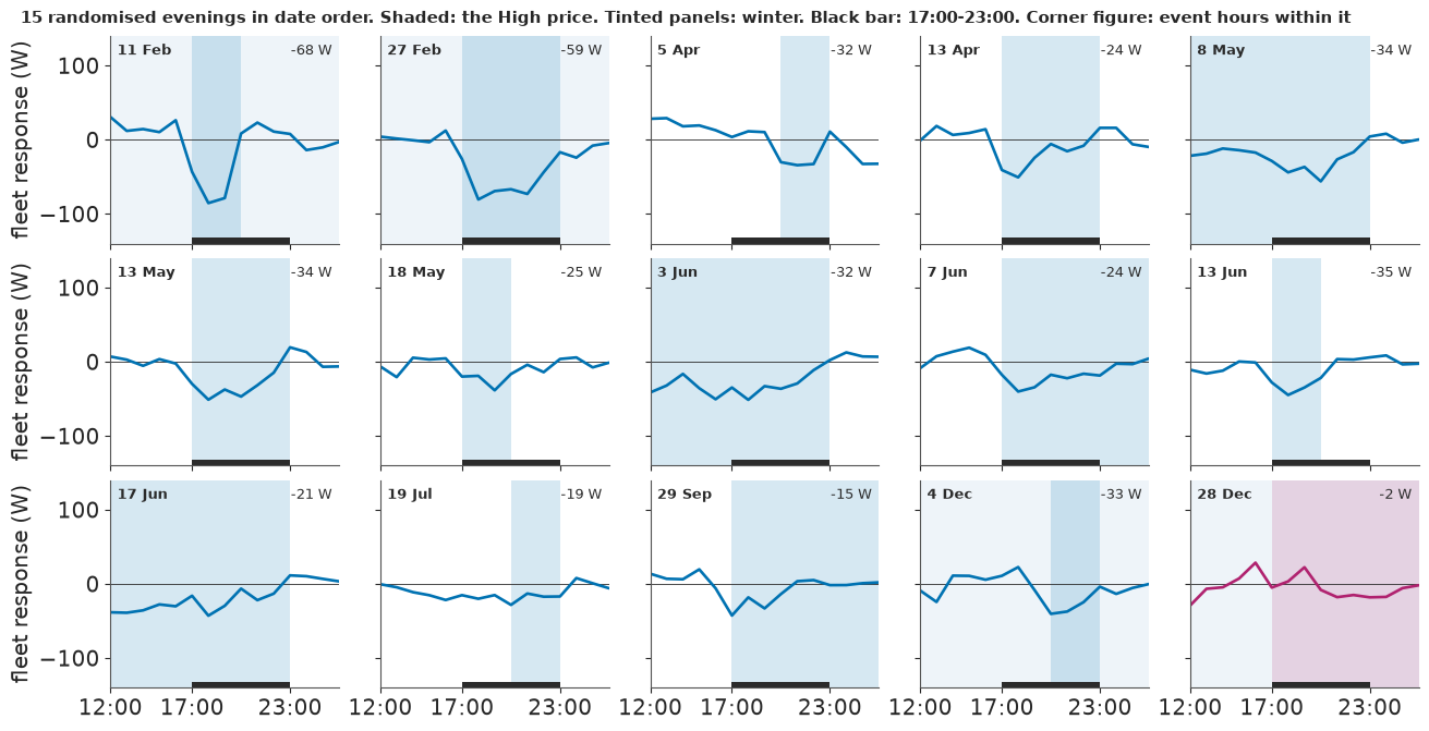
This is the main exhibit. Most panels show the same plain thing: load drops when the price starts and comes back when it ends. Summer evenings read -15 to -35 W on this baseline (season was not randomised, and on the whole window summer and winter both average about -40 W). The two February evenings are deep, at -68 and -59 W, and 4 December reads -33 W. 28 December shows almost nothing, about -2 W, with no step at 17:00. Every home saw the same evening, so that flat line is one observation, not a thousand.
table_w = home_tables["local"][:, cells.index]
sf_cells = cells.assign(
    W=np.nanmean(table_w, axis=0),
    se=np.nanstd(table_w, axis=0, ddof=1) / np.sqrt(np.isfinite(table_w).sum(axis=0)),
)[lambda f: f["effect"].str.startswith("SF")]
sf_cells = sf_cells.assign(
    priced=np.where(sf_cells["effect"].str.contains("High"), -1, 1) * sf_cells["W"],
)
sf_cells = sf_cells.assign(z=sf_cells["priced"] / sf_cells["se"])
print("SF cells from 15 November, 2013 month x band. priced: W in the direction the price asks for")
print(
    sf_cells[sf_cells["day"] >= "2013-11-15"]
    .sort_values("day")[["day", "effect", "start_hour", "event_hours", "W", "se", "priced", "z"]]
    .round(1)
    .to_string(index=False)
)
winter_cells = sf_cells[sf_cells["season"] == "gmt"]
after_19 = winter_cells["day"] > "2013-12-19"
print(
    f"After 19 December: {after_19.sum()} cells on {winter_cells[after_19]['day'].nunique()} events, mean {winter_cells[after_19]['priced'].mean():+.1f} W, "
    f"none past |z| {winter_cells[after_19]['z'].abs().max():.1f}. Other GMT cells: {(~after_19).sum()}, "
    f"mean {winter_cells[~after_19]['priced'].mean():+.1f} W, {(winter_cells[~after_19]['z'] >= 2).sum()} clear z = 2"
)
print(
    f"19 December, all Low, out of the analysis: {np.nanmean(fleet_response[(trial_day == '2013-12-19') & evening]):+.1f} W on the fleet mean, evening band"
)

types = evening_events.assign(
    W=local_means.to_numpy(), whole=np.nanmean(home_tables["plan"][:, evening_events.index], axis=0)
)
print("\nThe five evening event types, three repeats each in date order, W:")
print(
    types.groupby(["start_hour", "event_hours"])
    .agg(repeats=("W", lambda s: "  ".join(f"{v:.0f}" for v in s)), mean=("W", "mean"), whole_window_mean=("whole", "mean"))
    .round(1)
    .to_string()
)


def by_month(frame):
    return (pd.to_datetime(frame["day"]) - pd.Timestamp("2013-01-01")).dt.days.to_numpy() / 30.44


def trend(frame, key):
    fit = stats.linregress(by_month(frame), np.nanmean(home_tables[key][:, frame.index], axis=0))
    return f"{fit.slope:+.1f} ({fit.stderr:.1f})"


print("\nPost-hoc, W a month through 2013 (se between events); positive is a weakening cut, or a rising Low:")
print(
    pd.DataFrame(
        {
            name: {"2013 month x band": trend(frame, "local"), "whole window": trend(frame, "plan")}
            for name, frame in (
                ("SF High evening, 15", evening_events),
                ("same, 11 summer", evening_events[evening_events["season"] == "bst"]),
                ("SF Low evening, 15", cells[cells["effect"] == "SF Low evening"]),
                ("CM High evening, 17, not randomised", cells[cells["effect"] == "CM High evening"]),
            )
        }
    ).T.to_string()
)
others = types[types["day"] != DUD_DAY]
line = stats.linregress(by_month(others), others["W"])
spot = by_month(types[types["day"] == DUD_DAY])[0]
residual_sd = np.sqrt(((others["W"] - line.intercept - line.slope * by_month(others)) ** 2).sum() / (len(others) - 2))
leverage = 1 + 1 / len(others) + (spot - by_month(others).mean()) ** 2 / ((by_month(others) - by_month(others).mean()) ** 2).sum()
print(
    f"That trend, fitted to the other 14, predicts {line.intercept + line.slope * spot:.0f} W for 28 December "
    f"(prediction sd {residual_sd * np.sqrt(leverage):.0f} W), against {local_means[DUD_DAY]:.1f} W read"
)

default_evenings = evening & in_2013 & usable & (effect < 0) & ~np.isin(trial_day, event_days)
evening_mean = pd.Series(fleet_response[default_evenings]).groupby(trial_day[default_evenings]).mean()
is_gmt = (evening_mean.index < "2013-03-31") | (evening_mean.index >= "2013-10-27")
is_late = evening_mean.index >= "2013-12-20"
print(
    f"\nDefault evenings, fleet mean response, sd: GMT {evening_mean[is_gmt].std():.1f} W ({is_gmt.sum()} evenings), "
    f"of which 20-31 December {evening_mean[is_late].std():.1f} W ({is_late.sum()}); BST {evening_mean[~is_gmt].std():.1f} W"
)


clock_hour = hour_of_day + np.where(hour_of_day < 5, 24, 0)  # trial days run 05:00-05:00


def beside(event, first, last):
    """Fleet response in these clock hours of the event's trial day; NaN past the end of that day."""
    hours = (trial_day == event["day"]) & (clock_hour >= first) & (clock_hour < last)
    return np.nanmean(fleet_response[hours]) if hours.sum() == last - first else np.nan


before_w = np.array([beside(e, e["start_hour"] - 3, e["start_hour"]) for _, e in evening_events.iterrows()])
stops = evening_events["start_hour"] + evening_events["event_hours"]
after_w = np.array([beside(e, stop, stop + 3) for (_, e), stop in zip(evening_events.iterrows(), stops)])
print(
    f"Fleet mean in the 3 hours before an event {before_w.mean():+.1f} W (se {before_w.std(ddof=1) / np.sqrt(15):.1f}); "
    f"in the 3 hours after {np.nanmean(after_w):+.1f} W (se {np.nanstd(after_w, ddof=1) / np.sqrt(np.isfinite(after_w).sum()):.1f}, {np.isfinite(after_w).sum()} events)"
)
SF cells from 15 November, 2013 month x band. priced: W in the direction the price asks for
       day          effect  start_hour  event_hours     W   se  priced    z
2013-11-21  SF Low evening          17            3  78.4 13.2    78.4  6.0
2013-11-29    SF Low night          23            6  -2.4  5.0    -2.4 -0.5
2013-12-01  SF Low evening          17            3  88.6 15.3    88.6  5.8
2013-12-04 SF High evening          20            3 -32.6  8.6    32.6  3.8
2013-12-12    SF Low night          23            3  41.9  8.8    41.9  4.8
2013-12-22  SF Low evening          17           12  14.5 10.1    14.5  1.4
2013-12-22    SF Low night          17           12   1.3  3.9     1.3  0.3
2013-12-26  SF Low morning           8            3  -2.4 11.4    -2.4 -0.2
2013-12-28 SF High evening          17           12  -1.7 10.1     1.7  0.2
2013-12-28   SF High night          17           12  -4.2  4.1     4.2  1.0
After 19 December: 5 cells on 3 events, mean +3.8 W, none past |z| 1.4. Other GMT cells: 35, mean +54.0 W, 34 clear z = 2
19 December, all Low, out of the analysis: +45.6 W on the fleet mean, evening band

The five evening event types, three repeats each in date order, W:
                              repeats  mean  whole_window_mean
start_hour event_hours
11         12           -34  -32  -21 -29.2              -43.8
17         3            -68  -25  -35 -42.6              -52.8
           6            -59  -24  -34 -38.9              -49.5
           12            -24  -15  -2 -13.6              -25.7
20         3            -32  -19  -33 -27.9              -41.9

Post-hoc, W a month through 2013 (se between events); positive is a weakening cut, or a rising Low:
                                    2013 month x band whole window
SF High evening, 15                        +3.8 (1.1)   +3.6 (0.7)
same, 11 summer                            +2.9 (1.1)   +3.5 (1.0)
SF Low evening, 15                         +0.2 (2.2)   -0.9 (2.3)
CM High evening, 17, not randomised        +2.2 (0.8)   +0.4 (0.5)
That trend, fitted to the other 14, predicts -9 W for 28 December (prediction sd 16 W), against -1.7 W read

Default evenings, fleet mean response, sd: GMT 10.9 W (98 evenings), of which 20-31 December 12.2 W (7); BST 6.8 W
Fleet mean in the 3 hours before an event +4.6 W (se 2.3); in the 3 hours after -0.2 W (se 2.9, 12 events)
28 December is not alone. In the first table, signed so that positive is the way the price asked, every SF event after 19 December shows nothing: 5 cells on 3 events, mean about 4 W, none past 2 se, against about 54 W on the other 35 winter cells. That includes Low prices on 22 and 26 December, which should have raised load, while 19 December, priced Low all day, still responded. We found this after seeing the outcomes, so it is exploratory, but the question is a run of days.
Noise cannot explain it: a default winter evening varies by about 11 W, and late December by about 12 W, so a true -40 W reading as -2 W would take about 3.5 sd. Four explanations remain, and the data can test none of them properly:
- The signal was not sent, or not seen. Nothing in the release can tell.
- Christmas week. Homes may be away, or may not shift at that time of year.
- The event type. The 17:00, 12-hour event is the weakest of the five evening types (-24, -15 and -2 W) in the second table.
- A fade through 2013. SF High evenings weaken by about 4 W a month on either baseline, in summer alone too, while SF Low shows no trend; the other 14 evenings predict about -9 W (sd 16) for 28 December.
The last two were also found by looking. They matter because the four winter evenings are four different designs at the two ends of the trial, and every model below treats them as exchangeable, four draws from one distribution of winter evenings, which these data cannot check. Dropping 28 December would select on the outcome, so the rows without it below are a sensitivity, not a neutral alternative.
The last line checks the hours next to events: about +5 W (se 2) before and 0 W after, so there is no large anticipation or rebound on average, though single evenings differ.
M4: put the day in the model
A home's response on an evening is its group's usual effect, plus what was special about that day for every home, plus its own noise. Averaging over homes removes the noise, so we model event means:
$$\bar r_e \sim \text{Normal}\big(\mu_{c(e)} + v_e,\ \text{se}_e^2\big), \qquad v_e \sim \text{Normal}(0, \tau_e^2), \qquad \mu_c \sim N(0, 100), \quad \tau_e \sim \text{HalfNormal}(30).$$
Here $e$ runs over the 15 SF evenings, $c(e)$ is winter (4) or summer (11), and $\text{se}_e$ is the
between-home standard error, known from the table. One day spread $\tau_e$ serves both seasons,
because four events could never estimate their own; that says a winter evening varies as much as a
summer one, on evidence that is mostly summer. The CM evenings stay out, so the prior on $\tau_e$
matters more. A Student-t version on each home's cell, tried
first, again put nu at 2 and missed the mean.
def event_means(baseline="local", drop=(), kinds=("SF",)):
    """One row per High evening event: mean, between-home se and sd, and its group. SF only unless asked."""
    keep = cells["effect"].isin([f"{kind} High evening" for kind in kinds]) & ~cells["day"].isin(drop)
    frame = cells[keep].sort_values("day")
    r = home_tables[baseline][:, frame.index]
    seen = np.isfinite(r).sum(axis=0)
    out = pd.DataFrame(
        {
            "day": frame["day"].to_numpy(),
            "season": frame["season"].to_numpy(),
            "hours": frame["hours"].to_numpy(),
            "kind": frame["effect"].str[:2].to_numpy(),
            "mean": np.nanmean(r, axis=0),
            "sd": np.nanstd(r, axis=0, ddof=1),
            "homes": seen,
        }
    )
    out["se"] = out["sd"] / np.sqrt(seen)
    out["group"] = (out["kind"] == "CM").astype(int) * 2 + (out["season"] == "bst").astype(int)
    return out


def m4_model(frame, tau_scale=30.0, own_spread=False):
    """M4. With own_spread, the randomised winter evenings get a day spread of their own."""
    coords = {
        "group": GROUPS[: 4 if (frame["kind"] == "CM").any() else 2],
        "event": frame["day"].to_numpy(dtype=object),
        "spread": ("SF winter", "SF summer"),
    }
    with pm.Model(coords=coords) as model:
        mu = pm.Normal("mu", 0.0, 100.0, dims="group")
        v_raw = pm.Normal("v_raw", 0.0, 1.0, dims="event")
        if own_spread:
            tau_e = pm.HalfNormal("tau_e", tau_scale, dims="spread")
            scale = tau_e[(frame["group"].to_numpy() != 0).astype(int)]
        else:
            scale = tau_e = pm.HalfNormal("tau_e", tau_scale)
        v = pm.Deterministic("v", scale * v_raw, dims="event")
        pm.Normal(
            "r",
            mu[frame["group"].to_numpy()] + v,
            frame["se"].to_numpy(),
            observed=frame["mean"].to_numpy(),
            dims="event",
        )
    return model


def fit_m4(baseline="local", drop=(), tau_scale=30.0, seed=RANDOM_SEED, own_spread=False, frame=None):
    """Fit M4 and keep only what delivery needs. `tau` is the spread that applies to a winter evening."""
    frame = event_means(baseline, drop) if frame is None else frame
    trace = pm.sample(
        model=m4_model(frame, tau_scale, own_spread),
        chains=4,
        tune=1000,
        draws=1000,
        target_accept=0.99 if own_spread else 0.95,  # a spread on 4 events is a harder geometry: section 6
        cores=CHAINS_AT_ONCE,
        random_seed=seed,
        progressbar=False,
    )
    tau = trace.posterior["tau_e"]
    return {
        "frame": frame,
        "trace": trace,
        "mu": trace.posterior["mu"].values.reshape(-1, trace.posterior["mu"].sizes["group"]),
        "tau": (tau.sel(spread="SF winter") if own_spread else tau).values.ravel(),
        "sd": float(frame["sd"].median()),
        "divergences": int(trace.sample_stats["diverging"].values.sum()),
    }


def max_rhat(fit):
    hat = az.rhat(fit["trace"].posterior.to_dataset())
    hat = hat.to_dataset() if hasattr(hat, "to_dataset") else hat
    return max(float(hat[name].max()) for name in ("mu", "tau_e"))


def hour_weighted(baseline, days=None):
    picked = evening_events if days is None else evening_events[evening_events["day"].isin(days)]
    means = np.nanmean(home_tables[baseline][:, picked.index], axis=0)
    return float(np.average(means, weights=picked["hours"]))


winter_days = list(evening_events.loc[evening_events["season"] == "gmt", "day"])
summer_days = list(evening_events.loc[evening_events["season"] == "bst", "day"])
print(
    pd.DataFrame(
        {
            name: {
                "all 15 events": hour_weighted(baseline),
                "11 summer": hour_weighted(baseline, summer_days),
                "4 winter": hour_weighted(baseline, winter_days),
                "3 winter, no 28 Dec": hour_weighted(baseline, [d for d in winter_days if d != DUD_DAY]),
            }
            for name, baseline in (("2013, month x band", "local"), ("whole window", "plan"))
        }
    )
    .T.round(1)
    .to_string()
)
print(
    "Those are SF High evening means from the home x event table, weighted by hours; below, one row per kind of event, unweighted"
)
frame = event_means()
print(
    frame.groupby(["kind", "season"])
    .agg(
        events=("mean", "size"),
        mean_w=("mean", "mean"),
        between_events_sd=("mean", "std"),
        median_se=("se", "median"),
    )
    .round(1)
    .to_string()
)
prior_draw = pm.sample_prior_predictive(model=m4_model(frame), draws=2000, random_seed=RANDOM_SEED)
prior_r = prior_draw.prior_predictive["r"].values.ravel()
print(
    f"Prior predictive for an event mean: 5-95% {np.quantile(prior_r, 0.05):.0f} to {np.quantile(prior_r, 0.95):.0f} W, "
    f"against observed {frame['mean'].min():.0f} to {frame['mean'].max():.0f} W"
)

with stage("M4, 4 fits"):
    fits = {
        (baseline, label): fit_m4(baseline, drop)
        for baseline in ("local", "plan")
        for label, drop in (("all 4 winter events", ()), ("without 28 Dec", (DUD_DAY,)))
    }
main, main_x = fits[("local", "all 4 winter events")], fits[("local", "without 28 Dec")]
print(az.summary(main["trace"], var_names=["mu", "tau_e"], ci_kind="hdi", ci_prob=0.9, round_to=2).to_string())
print(
    f"Divergences: {main['divergences']}; tuning steps {main['trace'].posterior.attrs.get('tuning_steps', 'not recorded')}"
)
fit_view = {
    f"{'2013 month x band' if k[0] == 'local' else 'whole window'}, {k[1]}": {
        "SF winter": np.median(f["mu"][:, 0]),
        "5%": np.quantile(f["mu"][:, 0], 0.05),
        "95%": np.quantile(f["mu"][:, 0], 0.95),
        "SF summer": np.median(f["mu"][:, 1]),
        "tau_e": np.median(f["tau"]),
        "tau_e 5%": np.quantile(f["tau"], 0.05),
        "tau_e 95%": np.quantile(f["tau"], 0.95),
        "max r_hat": max_rhat(f),
        "divergences": f["divergences"],
    }
    for k, f in fits.items()
}
print(pd.DataFrame(fit_view).T.round(2).to_string())
                    all 15 events  11 summer  4 winter  3 winter, no 28 Dec
2013, month x band          -29.2      -26.7     -37.0                -54.6
whole window                -41.6      -42.2     -39.8                -55.3
Those are SF High evening means from the home x event table, weighted by hours; below, one row per kind of event, unweighted
             events  mean_w  between_events_sd  median_se
kind season
SF   bst         11   -26.8                7.0        6.0
     gmt          4   -40.3               29.8        9.4
Prior predictive for an event mean: 5-95% -176 to 171 W, against observed -68 to -2 W
                mean    sd  hdi90_lb  hdi90_ub  ess_bulk  ess_tail  r_hat  mcse_mean  mcse_sd
mu[SF winter] -39.25  7.85    -51.94    -26.45   1794.84   1849.94   1.00       0.19     0.17
mu[SF summer] -26.90  4.52    -34.09    -19.34   1067.71   1027.99   1.01       0.14     0.14
tau_e          11.49  4.30      4.72     18.25    697.85   1089.85   1.01       0.16     0.12
Divergences: 0; tuning steps 1000
                                        SF winter     5%    95%  SF summer  tau_e  tau_e 5%  tau_e 95%  max r_hat  divergences
2013 month x band, all 4 winter events     -39.46 -51.91 -26.34     -26.83  11.13      5.19      19.12       1.01          0.0
2013 month x band, without 28 Dec          -50.51 -61.11 -39.88     -26.89   5.29      0.78      11.88       1.00          0.0
whole window, all 4 winter events          -41.78 -53.04 -30.69     -42.22   7.24      1.10      15.05       1.01          0.0
whole window, without 28 Dec               -52.18 -62.85 -41.04     -42.41   3.90      0.40      10.00       1.00          0.0
Hour-weighted, the four winter evenings average -37 W on the 2013 baseline and -40 W on the whole window, about -55 W without 28 December. Summer evenings sit close together (about -27 W, spread 7 W); winter's four read -68, -59, -33 and -2 W (spread 30 W). The prior predictive comfortably covers them.
The fit is clean, with no divergences and r_hat at most 1.01. SF winter comes out near -39 W (90% interval -52 to -26), -42 W on the whole window, and about -51 W without 28 December. The day spread $\tau_e$ is about 11 W (5 to 19), or 7 W on the whole window. With so few events, three more looks: the prior, a predictive check, and a winter spread of its own.
with stage("M4, tau_e prior"):
    sensitivity = {scale: fit_m4(tau_scale=scale) for scale in (10.0, 100.0)}
sensitivity[30.0] = main
print(
    pd.DataFrame(
        {
            f"HalfNormal({scale:.0f})": {
                "tau_e median": np.median(f["tau"]),
                "tau_e 5%": np.quantile(f["tau"], 0.05),
                "tau_e 95%": np.quantile(f["tau"], 0.95),
                "SF winter median": np.median(f["mu"][:, 0]),
                "SF winter sd": f["mu"][:, 0].std(),
            }
            for scale, f in sorted(sensitivity.items())
        }
    )
    .round(1)
    .to_string()
)

check_rng = np.random.default_rng(RANDOM_SEED + 2)
frame_main = main["frame"]
new_day = (
    main["mu"][:, frame_main["group"].to_numpy()]
    + check_rng.normal(0, 1, (4000, len(frame_main))) * main["tau"][:, None]
)
new_mean = new_day + check_rng.normal(0, 1, new_day.shape) * frame_main["se"].to_numpy()
low, high = np.quantile(new_mean, [0.05, 0.95], axis=0)
inside = (frame_main["mean"].to_numpy() >= low) & (frame_main["mean"].to_numpy() <= high)
print(
    f"Check with each day's effect redrawn: {inside.sum()} of {len(frame_main)} event means inside their 90% band. Outside: "
    f"{', '.join(frame_main['day'][~inside])}"
)

with stage("M4, own winter spread"):
    own, own_x = fit_m4(own_spread=True), fit_m4(drop=(DUD_DAY,), own_spread=True)
    own_wide = fit_m4(own_spread=True, tau_scale=60.0)
print(
    pd.DataFrame(
        {
            name: {
                "SF winter median": np.median(f["mu"][:, 0]),
                "5%": np.quantile(f["mu"][:, 0], 0.05),
                "95%": np.quantile(f["mu"][:, 0], 0.95),
                "winter tau_e median": np.median(f["tau"]),
                "tau_e 5%": np.quantile(f["tau"], 0.05),
                "tau_e 95%": np.quantile(f["tau"], 0.95),
                "max r_hat": max_rhat(f),
                "divergences": f["divergences"],
            }
            for name, f in (
                ("own spread, 4 events", own),
                ("own spread, without 28 Dec", own_x),
                ("own spread, 4 events, HalfNormal(60)", own_wide),
            )
        }
    )
    .T.round(2)
    .to_string()
)

fig, ax = plt.subplots(figsize=(12.5, 5), layout="constrained")
bst = pd.date_range("2013-03-31", "2013-10-27")
ax.axvspan(bst[0], bst[-1], color="#f1f0ec", lw=0, zorder=0)
ax.axhline(0, color=INK, lw=0.8)
post_event = main["mu"][:, frame_main["group"].to_numpy()] + main["trace"].posterior["v"].values.reshape(4000, -1)
medians, lo, hi = np.median(post_event, axis=0), *np.quantile(post_event, [0.05, 0.95], axis=0)
winter_raw = frame_main.query("group == 0")["mean"]
print(
    f"28 December: raw {frame_main.loc[frame_main['day'] == DUD_DAY, 'mean'].iloc[0]:.1f} W, shared-spread estimate "
    f"{medians[(frame_main['day'] == DUD_DAY).to_numpy()][0]:.1f} W. Winter mean: sd {main['mu'][:, 0].std():.1f} W in the model, "
    f"raw se of the four {winter_raw.std() / 2:.1f} W"
)
dates = pd.to_datetime(frame_main["day"])
ax.vlines(dates, lo, hi, color=SF_C, lw=1.6, alpha=0.65)
ax.scatter(dates, medians, s=55, color=SF_C, edgecolor="w", lw=1, zorder=3, label="SF evening, randomised")
ax.scatter(dates, frame_main["mean"], s=26, marker="x", color=INK, lw=1, zorder=4, label="raw mean of the evening")
dud = (frame_main["day"] == DUD_DAY).to_numpy()
ax.annotate(
    "28 December: raw mean near 0,\npulled towards its group",
    (dates[dud].iloc[0], medians[dud][0]),
    xytext=(-175, 22),
    textcoords="offset points",
    fontsize=9.5,
    color=INK,
    arrowprops=dict(arrowstyle="-", color=DUD_C, lw=1),
)
ax.scatter(dates[dud], medians[dud], s=90, facecolor="w", edgecolor=DUD_C, lw=2.2, zorder=3)
ax.annotate("BST months: summer evenings", (pd.Timestamp("2013-07-01"), 8), fontsize=9.5, color=INK, ha="center")
ax.set(ylabel="response on the evening (W), 90% interval", ylim=(-85, 18))
ax.xaxis.set_major_formatter(mdates.ConciseDateFormatter(ax.xaxis.get_major_locator()))
ax.legend(loc="lower right", fontsize=9, ncols=2)
ax.set_title(
    "Each mark is one evening that every home shared. A shared day spread pulls the two winter extremes hard",
    loc="left",
    fontsize=11,
);
                  HalfNormal(10)  HalfNormal(30)  HalfNormal(100)
tau_e median                 9.6            11.1             11.0
tau_e 5%                     3.7             5.2              4.8
tau_e 95%                   16.0            19.1             19.3
SF winter median           -39.2           -39.5            -39.1
SF winter sd                 6.8             7.9              7.9
Check with each day's effect redrawn: 14 of 15 event means inside their 90% band. Outside: 2013-12-28
                                      SF winter median     5%    95%  winter tau_e median  tau_e 5%  tau_e 95%  max r_hat  divergences
own spread, 4 events                            -39.61 -63.84 -13.60                27.76     14.39      50.74       1.01          0.0
own spread, without 28 Dec                      -50.52 -74.70 -24.45                18.51      3.53      47.59       1.01          0.0
own spread, 4 events, HalfNormal(60)            -37.93 -71.63  -5.55                34.36     15.85      76.76       1.02          0.0
28 December: raw -1.7 W, shared-spread estimate -19.9 W. Winter mean: sd 7.9 W in the model, raw se of the four 14.9 W
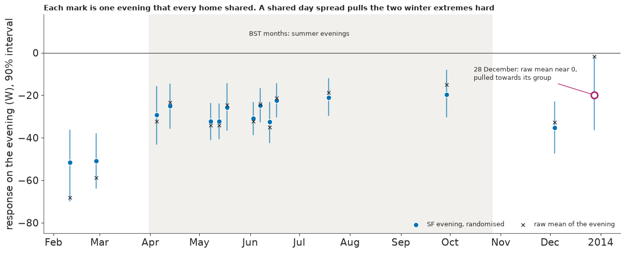
The prior matters a little: HalfNormal(10) gives a spread of about 10 W, and HalfNormal(100) changes almost nothing.
The check spoils it. Redraw each day's effect: 14 of 15 event means fall inside their 90% band, and the one outside is 28 December, one of the four evenings that matter. A $\tau_e$ set mostly by summer treats it as ordinary noise, pulls it from -2 to about -20 W, and gives the winter mean an sd of 8 W where the four evenings alone have a raw standard error of 15 W.
With a winter spread of its own, the mean barely moves (near -40 W) but its 90% interval opens to
about -64 to -14 W, with a winter $\tau_e$ near 28 W (14 to 51). Under a HalfNormal(60) prior it
becomes 34 W and the interval about -72 to -6 W. These fits are funnels with four events in the neck,
so they run at target_accept=0.99; none diverges, but four end at r_hat 1.011-1.021 (listed in
section 7), and their figures are rounded with that in mind. Four evenings cannot bound their own
spread. That is a fact about the evidence, so both versions go forward: the shared spread is the
narrow reading, the own spread the wide one.
7 · How many homes? Failure 5
On a new winter evening with $N$ homes offered and a fraction $a$ accepting, the total cut is
$$\text{cut} = N a\,\big(-\mu - v\big) + \sqrt{N a}\;s\,\varepsilon, \qquad v \sim N(0, \tau_e^2),$$
with $s$ the between-home sd of an evening's response. More homes shrink the second term relative to the first and do nothing to $\mu$ or $v$: no enrolment averages out a shared bad evening. "1 MW" is a mean over an event's priced hours, and a new evening is one more draw from the old ones.
The target and the acceptance rate are the planner's. The 24% used here is the "uptake" in the trial's slides, whose denominator we could not trace, so it is an assumption. We count four ways: homes only, as a fleet-wide standard error does; plus the uncertainty in $\mu$; plus a new evening's $v$; and with winter's own day spread. Last, no model at all: the next evening is one of the four, equally likely.
Z_DAY, Z_HOMES = np.random.default_rng(RANDOM_SEED + 3).normal(0, 1, (2, 4000))


def chance(fit, group, offers, acceptance=ACCEPTANCE, target_mw=1.0, shared=True):
    """P(total cut >= target) on one new evening, for scalar or array offers."""
    homes = np.asarray(offers, float)[..., None] * acceptance
    day = fit["tau"] * Z_DAY if shared else 0.0
    cut = -homes * (fit["mu"][:, group] + day) - np.sqrt(homes) * fit["sd"] * Z_HOMES
    return (cut >= target_mw * 1e6).mean(axis=-1)


def counting_homes(baseline="local", drop=(), offers=1e5, acceptance=ACCEPTANCE, target_mw=1.0):
    """The fleet treated as the sample: every home an independent draw, the four evenings forgotten."""
    frame = event_means(baseline, drop)
    picked = frame[frame["group"] == 0]
    keep = cells["day"].isin(picked["day"]) & (cells["effect"] == "SF High evening")
    per_home = np.nanmean(home_tables[baseline][:, cells[keep].index], axis=1)
    mean, sd = np.nanmean(per_home), np.nanstd(per_home, ddof=1)
    se = sd / np.sqrt(np.isfinite(per_home).sum())
    homes = np.asarray(offers, float) * acceptance
    return stats.norm.cdf((-homes * mean - target_mw * 1e6) / np.sqrt(homes**2 * se**2 + homes * sd**2))


def face_value(baseline="local", drop=(), offers=1e5, acceptance=ACCEPTANCE, target_mw=1.0):
    """No model of the day: the next evening is one of the observed evenings, equally likely."""
    frame = event_means(baseline, drop)
    means = frame[frame["group"] == 0]["mean"].to_numpy()
    homes = np.asarray(offers, float)[..., None] * acceptance
    return (-homes * means >= target_mw * 1e6).mean(axis=-1)


OFFERS = (50_000, 100_000, 200_000)
with stage("M4, one row borrowing CM"):
    borrowed = fit_m4(frame=event_means(kinds=("SF", "CM")))  # never feeds a headline: gate P5 failed
rows = {}
for (baseline, label), fit in fits.items():
    name = f"SF winter, {'2013 month x band' if baseline == 'local' else 'whole window'}, {label}"
    rows[name] = {f"{o:,}": float(chance(fit, 0, o)) for o in OFFERS}
rows["SF winter, own day spread, all 4"] = {f"{o:,}": float(chance(own, 0, o)) for o in OFFERS}
rows["SF winter, own day spread, without 28 Dec"] = {f"{o:,}": float(chance(own_x, 0, o)) for o in OFFERS}
rows["SF winter, day spread borrowed from 17 CM evenings: NOT randomised, outside every headline range"] = {
    f"{o:,}": float(chance(borrowed, 0, o)) for o in OFFERS
}
rows["CM winter, 2013 month x band: NOT randomised, outside every headline range"] = {
    f"{o:,}": float(chance(borrowed, 2, o)) for o in OFFERS
}
delivery_table = pd.DataFrame(rows).T
cm_placebo = f"{placebo['CM High evening']['mean_w']:+.1f} W, gate failed"
print(f"P(at least 1 MW off one winter evening), {ACCEPTANCE:.0%} acceptance (an assumption), by homes offered")
print(
    delivery_table.round(2)
    .assign(**{"CM placebo": [""] * (len(delivery_table) - 2) + [cm_placebo] * 2})
    .to_string()
)
ways = {
    "counting homes": [float(counting_homes(offers=o)) for o in OFFERS],
    "adding uncertainty in mu": [float(chance(main, 0, o, shared=False)) for o in OFFERS],
    "adding a new evening's v": [float(chance(main, 0, o)) for o in OFFERS],
    "winter with its own day spread": [float(chance(own, 0, o)) for o in OFFERS],
    "the 4 evenings at face value": [float(face_value(offers=o)) for o in OFFERS],
}
print("\nFour ways of counting, then no model at all, 2013 month x band, all 4 events:")
print(pd.DataFrame(ways, index=[f"{o:,}" for o in OFFERS]).T.round(2).to_string())
dud_read = {b: float(event_means(b).set_index("day").loc[DUD_DAY, "mean"]) for b in ("local", "plan")}
print(
    "\n28 December reaches 1 MW at "
    + ", ".join(
        f"{-1e6 / w:,.0f} accepting homes, {-1e6 / w / ACCEPTANCE:,.0f} offers ({w:.1f} W, {name})"
        for w, name in ((dud_read["local"], "2013 month x band"), (dud_read["plan"], "whole window"))
    )
)
P(at least 1 MW off one winter evening), 24% acceptance (an assumption), by homes offered
                                                                                                  50,000  100,000  200,000            CM placebo
SF winter, 2013 month x band, all 4 winter events                                                   0.01     0.42     0.91
SF winter, 2013 month x band, without 28 Dec                                                        0.00     0.85     1.00
SF winter, whole window, all 4 winter events                                                        0.00     0.49     0.97
SF winter, whole window, without 28 Dec                                                             0.00     0.90     1.00
SF winter, own day spread, all 4                                                                    0.10     0.46     0.72
SF winter, own day spread, without 28 Dec                                                           0.10     0.67     0.89
SF winter, day spread borrowed from 17 CM evenings: NOT randomised, outside every headline range    0.00     0.40     0.95  +13.2 W, gate failed
CM winter, 2013 month x band: NOT randomised, outside every headline range                          0.00     0.81     1.00  +13.2 W, gate failed

Four ways of counting, then no model at all, 2013 month x band, all 4 events:
                                50,000  100,000  200,000
counting homes                    0.00     0.42     1.00
adding uncertainty in mu          0.00     0.38     0.99
adding a new evening's v          0.01     0.42     0.91
winter with its own day spread    0.10     0.46     0.72
the 4 evenings at face value      0.00     0.50     0.75

28 December reaches 1 MW at 581,604 accepting homes, 2,423,350 offers (-1.7 W, 2013 month x band), 115,133 accepting homes, 479,719 offers (-8.7 W, whole window)
At 100,000 offers (24,000 homes, needing about 42 W each) every version sits near an even chance with all four evenings (0.38-0.50) and moves to 0.7-0.9 without 28 December; neither row should be quoted alone. At 50,000 nothing passes 0.1.
The fifth failure is at 200,000 offers. Counting homes says 1.00, and adding the uncertainty in $\mu$ still says 0.99. A new evening's $v$ brings it to 0.91 (0.97 on the whole window); winter's own spread gives 0.72, and the four evenings at face value 0.75. Each extra home shrinks only the noise that was already small. At face value, 28 December's -1.7 W would need about 2.4 million offers to reach 1 MW (480,000 on the whole-window baseline), so one evening in four falls short at any realistic scale.
The last two delivery rows borrow the placed CM evenings, beside a failed placebo, and are not part of the answer: CM winter's 0.81 at 100,000 offers rests on days nobody randomised.
grid = np.geomspace(1e4, 1e6, 160)
fig, axes = plt.subplots(1, 2, figsize=(12.5, 4.9), sharey=True, layout="constrained")
for ax, fit, wide, drop, title in zip(
    axes,
    (main, main_x),
    (own, own_x),
    ((), (DUD_DAY,)),
    ("All 4 randomised winter evenings", "Without 28 December: 3 evenings"),
):
    ax.axvline(1e5, color="#c7c7c7", lw=1)
    ax.plot(
        grid,
        counting_homes(drop=drop, offers=grid),
        color=MUTED,
        lw=2,
        ls="--",
        label="counting homes: the fleet as the sample",
    )
    ax.plot(grid, chance(fit, 0, grid), color=SKY, lw=2.4, ls="-.", label="M4, one day spread shared by all events")
    ax.plot(grid, chance(wide, 0, grid), color=SF_C, lw=2.6, label="M4, winter's own day spread")
    ax.step(
        grid,
        face_value(drop=drop, offers=grid),
        where="post",
        color=DUD_C,
        lw=1.8,
        label="the observed evenings at face value",
    )
    ax.set_title(title, fontsize=10.5)
    ax.tick_params(labelsize=10)
    ax.set(
        xscale="log",
        xlabel=f"homes offered, at {ACCEPTANCE:.0%} acceptance (an assumption)",
        ylim=(-0.02, 1.04),
        xlim=(1e4, 1e6),
    )
    ax.xaxis.set_major_formatter(FuncFormatter(lambda v, _: f"{v / 1000:,.0f}k"))
    ax.set_xticks([1e4, 5e4, 1e5, 2e5, 5e5, 1e6])
axes[0].set_ylabel("chance of at least 1 MW on one evening")
fig.legend(*axes[0].get_legend_handles_labels(), loc="outside lower center", ncols=4, fontsize=9.5)
fig.suptitle(
    "Homes buy margin, not certainty. With 28 December in the record, face value stops at 3 in 4 from about 130k offers",
    x=0.01,
    ha="left",
    fontsize=11,
);
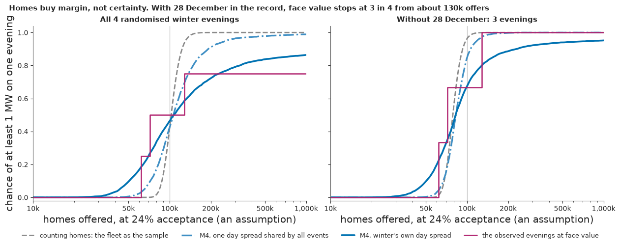
The dashed "counting homes" curve is a cliff; the own-spread curve and the face-value steps flatten well below 1. Next, the chance for any acceptance under winter's own spread, and the homes needed.
offers_axis = np.geomspace(1e4, 6e5, 90)
acceptance_axis = np.linspace(0.05, 0.6, 70)
fig, axes = plt.subplots(1, 2, figsize=(12.5, 4.9), sharey=True, layout="constrained")
for ax, fit, title in zip(
    axes,
    (own, own_x),
    ("All 4 randomised winter evenings, own day spread", "Without 28 December: 3 evenings, own day spread"),
):
    surface = np.array([[float(chance(fit, 0, o, acceptance=a)) for o in offers_axis] for a in acceptance_axis])
    filled = ax.contourf(offers_axis, acceptance_axis, surface, levels=np.linspace(0, 1, 11), cmap="Blues")
    lines = ax.contour(
        offers_axis, acceptance_axis, surface, levels=[0.5, 0.8, 0.95], colors=[INK, "white", "white"], linewidths=1.3
    )
    ax.clabel(lines, fmt=lambda v: f"P = {v:.2f}", fontsize=9)
    ax.axhline(ACCEPTANCE, color=DUD_C, lw=1.4, ls="--")
    ax.annotate(
        "24%: an assumption, no traced source",
        (1.1e4, ACCEPTANCE),
        xytext=(0, 4),
        textcoords="offset points",
        fontsize=8.8,
        color=INK,
    )
    ax.set_title(title, fontsize=10.5)
    ax.tick_params(labelsize=10)
    ax.set(xscale="log", xlabel="homes offered")
    ax.xaxis.set_major_formatter(FuncFormatter(lambda v, _: f"{v / 1000:,.0f}k"))
    ax.set_xticks([1e4, 3e4, 1e5, 3e5, 6e5])
axes[0].set_ylabel("share who accept: the planner's input")
fig.colorbar(filled, ax=axes, shrink=0.85, label="chance of at least 1 MW on one evening")
fig.suptitle(
    "The planner's map. Pick an acceptance you can defend, then read off the offers", x=0.01, ha="left", fontsize=11
)


def homes_needed(fit, target_mw, probability):
    """Accepting homes needed for this chance, on a fine grid."""
    homes = np.geomspace(1e3, 4e6, 500)
    p = chance(fit, 0, homes, acceptance=1.0, target_mw=target_mw)
    reached = np.flatnonzero(p >= probability)
    return float(homes[reached[0]]) if reached.size else float("nan")


need = pd.DataFrame(
    {
        f"{target} MW, {label}": {f"P = {p}": homes_needed(fit, target, p) for p in (0.5, 0.8, 0.95)}
        for label, fit in (
            ("shared spread, all 4", main),
            ("own spread, all 4", own),
            ("own spread, no 28 Dec", own_x),
        )
        for target in (0.5, 1.0, 2.0)
    }
).T
print(
    "Accepting homes needed on one winter evening (divide by the acceptance rate for offers; NaN: not reached by 4 million):"
)
print(need.round(-2).to_string());
Accepting homes needed on one winter evening (divide by the acceptance rate for offers; NaN: not reached by 4 million):
                               P = 0.5   P = 0.8  P = 0.95
0.5 MW, shared spread, all 4   12900.0   18000.0   31200.0
1.0 MW, shared spread, all 4   26000.0   35600.0   62700.0
2.0 MW, shared spread, all 4   51400.0   71600.0  126100.0
0.5 MW, own spread, all 4      12900.0   38700.0       NaN
1.0 MW, own spread, all 4      26000.0   79200.0       NaN
2.0 MW, own spread, all 4      51400.0  156500.0       NaN
0.5 MW, own spread, no 28 Dec   9900.0   15500.0  108600.0
1.0 MW, own spread, no 28 Dec  19900.0   31200.0  207600.0
2.0 MW, own spread, no 28 Dec  40000.0   61700.0  424200.0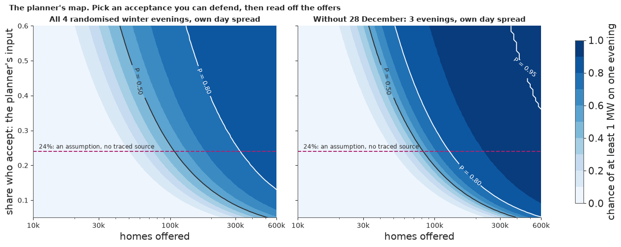
With all four evenings, an even chance of 1 MW needs about 26,000 accepting homes (108,000 offers at 24%). An 80% chance needs about 36,000 homes under a shared spread and about 79,000 (330,000 offers) under winter's own, where the curve is so flat that this figure moves between runs; 95% is never reached under winter's own spread. Without 28 December, 80% needs about 31,000 homes. For comparison, the trial's published figures give about 20,000 homes at the CM peak's 50 W and 33,000 at SF's 30 W.
So the answer hinges on a choice the data cannot make. Take the four evenings at face value and one in four falls short at any enrolment; let winter vary smoothly and the chance creeps from 0.72 at 200,000 offers to about 0.8 near 330,000. The map gives the same answer for any acceptance the planner can defend.
How much rests on each evening, and on what counts as the peak
Four checks made after seeing the results: drop each winter evening in turn; borrow the CM evenings for the day spread; treat the share of dead evenings as an input; and look at the hours a planner calls the peak.
leave_out, left_fits = {}, {}
with stage("M4, each evening left out"):
    for day in winter_days:
        pair = (main_x, own_x) if day == DUD_DAY else (fit_m4(drop=(day,)), fit_m4(drop=(day,), own_spread=True))
        if day != DUD_DAY:
            left_fits[f"shared, without {day}"], left_fits[f"own, without {day}"] = pair
        leave_out[f"without {pd.Timestamp(day):%-d %b}"] = {
            "shared, 100,000": float(chance(pair[0], 0, 100_000)),
            "own, 100,000": float(chance(pair[1], 0, 100_000)),
            "shared, 200,000": float(chance(pair[0], 0, 200_000)),
            "own, 200,000": float(chance(pair[1], 0, 200_000)),
            "SF winter median (shared)": np.median(pair[0]["mu"][:, 0]),
        }
print("Leave one winter evening out, P(1 MW):")
print(pd.DataFrame(leave_out).T.round(2).to_string())
print(
    f"\nDay spread with 17 CM evenings borrowed, NOT randomised, CM placebo {cm_placebo}: tau_e {np.median(borrowed['tau']):.1f} W "
    f"against {np.median(main['tau']):.1f} W on the 15 SF evenings; P(1 MW) {float(chance(borrowed, 0, 100_000)):.2f} at 100,000 offers, "
    f"{float(chance(borrowed, 0, 200_000)):.2f} at 200,000, against {float(chance(main, 0, 100_000)):.2f} and {float(chance(main, 0, 200_000)):.2f}"
)

gmt_days = ((days_2013 < "2013-03-31") | (days_2013 >= "2013-10-27")).sum()
fortnight = ((days_2013 >= "2013-12-20") | (days_2013 <= "2013-01-02")).sum()
print(f"\nA share w of winter evenings deliver nothing, the rest follow the 3-evening fits (own to shared spread):")
print(
    pd.DataFrame(
        {
            f"w = {w:.0%}{', post-hoc' if w < 0.25 else ''}": {
                "ceiling": f"{1 - w:.2f}",
                **{
                    f"{o:,} offers": f"{(1 - w) * float(chance(own_x, 0, o)):.2f}-{(1 - w) * float(chance(main_x, 0, o)):.2f}"
                    for o in (100_000, 200_000)
                },
            }
            for w in (fortnight / gmt_days, 0.25)
        }
    ).T.to_string()
)
print(
    f"w = {fortnight / gmt_days:.0%} is {fortnight} of {gmt_days} GMT days, 20 December to 2 January, a window drawn after seeing the data; "
    "25% is 1 in 4 evenings"
)

flat_winter = (wall.month <= 2) & (wall.dayofweek < 5) & in_2013
flat_hours = pd.Series(1000 * panel_kw[flat_winter]).groupby(hour_of_day[flat_winter]).mean()
print("\nFlat-home load, Jan-Feb 2013 weekdays, W by wall hour:", flat_hours.loc[16:21].round(0).astype(int).to_dict())
evening_load = pd.Series(1000 * panel_kw[evening & in_2013]).groupby(trial_day[evening & in_2013]).mean()
winter_load = evening_load[(evening_load.index < "2013-03-31") | (evening_load.index >= "2013-10-27")]
print(
    f"Highest-load evenings of 2013: {sum(d[5:7] == '01' for d in evening_load.nlargest(10).index)} of 10 in January, and no randomised "
    f"evening High event falls in January. 28 December sits at percentile {(winter_load < winter_load[DUD_DAY]).mean():.0%} of winter evenings, "
    f"and the highest evening from 20-31 December at {(winter_load < winter_load[winter_load.index >= '2013-12-20'].max()).mean():.0%}"
)


def peak_frame():
    """event_means with each mean replaced by the fleet response at 18:00-20:00, for events priced in both hours."""
    frame = event_means()
    peak = (hour_of_day >= 18) & (hour_of_day < 20)
    values = []
    for _, row in frame.iterrows():
        hours = peak & (trial_day == row["day"])
        priced = (effect[hours] == EFFECTS.index(f"{row['kind']} High evening")).sum()
        values.append(np.nanmean(fleet_response[hours]) if priced == 2 else np.nan)
    return frame.assign(mean=values).dropna(subset=["mean"])


peak_events = peak_frame()
with stage("M4, peak hours"):
    peak_fits = {
        "shared, all": fit_m4(frame=peak_events),
        "own, all": fit_m4(frame=peak_events, own_spread=True),
        "shared, without 28 Dec": fit_m4(frame=peak_events[peak_events["day"] != DUD_DAY]),
        "own, without 28 Dec": fit_m4(frame=peak_events[peak_events["day"] != DUD_DAY], own_spread=True),
    }
four_evenings = pd.DataFrame(
    {
        pd.Timestamp(day).strftime("%-d %b"): {
            "event hours (W)": local_means[day],
            "fleet, 18:00-20:00 (W)": np.nanmean(fleet_response[(trial_day == day) & (hour_of_day >= 18) & (hour_of_day < 20)]),
            "priced at 18:00-20:00": day in set(peak_events["day"]),
        }
        for day in winter_days
    }
).T
print(four_evenings.to_string())
same_fits = dict(zip(peak_fits, (main, own, main_x, own_x)))
every_fit = {
    **{f"shared, {k[0]}, {k[1]}": f for k, f in fits.items()},
    "shared, HalfNormal(10)": sensitivity[10.0],
    "shared, HalfNormal(100)": sensitivity[100.0],
    "own, all": own,
    "own, without 28 Dec": own_x,
    "own, HalfNormal(60)": own_wide,
    **left_fits,
    **{f"peak hours, {k}": f for k, f in peak_fits.items()},
}
hats = {name: max_rhat(f) for name, f in every_fit.items()}
own_fits = [f for name, f in every_fit.items() if "own" in name]
print(
    f"The {len(every_fit)} M4 fits on SF evenings: {sum(f['divergences'] for f in every_fit.values())} divergences, "
    f"{sum(f['divergences'] for f in own_fits)} of them in the {len(own_fits)} own-spread fits at target_accept=0.99. "
    f"Fits over r_hat 1.01: { {k: round(v, 3) for k, v in hats.items() if v > 1.01} or 'none'}. "
    f"The one CM-borrowing row: {borrowed['divergences']} divergences, r_hat {max_rhat(borrowed):.2f}"
)
print(
    pd.DataFrame(
        {
            name: {
                "priced hours, 100,000": float(chance(same_fits[name], 0, 100_000)),
                "18:00-20:00, 100,000": float(chance(fit, 0, 100_000)),
                "priced hours, 200,000": float(chance(same_fits[name], 0, 200_000)),
                "18:00-20:00, 200,000": float(chance(fit, 0, 200_000)),
            }
            for name, fit in peak_fits.items()
        }
    )
    .T.round(2)
    .to_string()
)
winter_peaks = peak_events.query("group == 0")["mean"].to_numpy()
print(
    f"At face value, 100,000 offers: {(-24_000 * winter_peaks >= 1e6).sum()} of {len(winter_peaks)} evenings at 18:00-20:00, "
    f"{(-24_000 * frame_main.query('group == 0')['mean'] >= 1e6).sum()} of 4 over priced hours"
)
Leave one winter evening out, P(1 MW):
                shared, 100,000  own, 100,000  shared, 200,000  own, 200,000  SF winter median (shared)
without 11 Feb             0.22          0.35             0.83          0.62                     -32.19
without 27 Feb             0.20          0.38             0.83          0.63                     -31.87
without 4 Dec              0.51          0.49             0.92          0.72                     -42.15
without 28 Dec             0.85          0.67             1.00          0.89                     -50.51

Day spread with 17 CM evenings borrowed, NOT randomised, CM placebo +13.2 W, gate failed: tau_e 8.4 W against 11.1 W on the 15 SF evenings; P(1 MW) 0.40 at 100,000 offers, 0.95 at 200,000, against 0.42 and 0.91

A share w of winter evenings deliver nothing, the rest follow the 3-evening fits (own to shared spread):
                 ceiling 100,000 offers 200,000 offers
w = 9%, post-hoc    0.91      0.61-0.77      0.81-0.91
w = 25%             0.75      0.51-0.64      0.66-0.75
w = 9% is 14 of 155 GMT days, 20 December to 2 January, a window drawn after seeing the data; 25% is 1 in 4 evenings

Flat-home load, Jan-Feb 2013 weekdays, W by wall hour: {16: 615, 17: 740, 18: 818, 19: 813, 20: 771, 21: 707}
Highest-load evenings of 2013: 8 of 10 in January, and no randomised evening High event falls in January. 28 December sits at percentile 17% of winter evenings, and the highest evening from 20-31 December at 45%
event hours (W) fleet, 18:00-20:00 (W) priced at 18:00-20:00 11 Feb -68.126151 -82.010744 True 27 Feb -58.793008 -74.880279 True 4 Dec -32.623915 7.165794 False 28 Dec -1.719383 12.846456 True
The 19 M4 fits on SF evenings: 0 divergences, 0 of them in the 8 own-spread fits at target_accept=0.99. Fits over r_hat 1.01: {'own, all': 1.013, 'own, HalfNormal(60)': 1.021, 'own, without 2013-12-04': 1.011, 'peak hours, own, all': 1.011}. The one CM-borrowing row: 0 divergences, r_hat 1.00
                        priced hours, 100,000  18:00-20:00, 100,000  priced hours, 200,000  18:00-20:00, 200,000
shared, all                              0.42                  0.57                   0.91                  0.83
own, all                                 0.46                  0.53                   0.72                  0.70
shared, without 28 Dec                   0.85                  1.00                   1.00                  1.00
own, without 28 Dec                      0.67                  0.94                   0.89                  0.98
At face value, 100,000 offers: 2 of 3 evenings at 18:00-20:00, 2 of 4 over priced hours
One evening swings it both ways. Without 28 December, 100,000 offers reads 0.85 or 0.67; without either February evening, about 0.2 (shared spread) or 0.35-0.38 (own). 28 December is not the only sensitivity, just the one with a story. Borrowing CM moves the shared spread from 11 to 8 W and 200,000 offers from 0.91 to 0.95, which shows that leaving those placed evenings out costs little.
How often is an evening dead? One in four is the raw count, with a 95% interval from under 1% to about 81%. If dead evenings were confined to a Christmas fortnight (20 December to 2 January, about 9% of winter days), the ceiling would be 0.91 and 200,000 offers would read about 0.8-0.9. That window was drawn after seeing the data, so it is a sensitivity, not a finding. The planner might also ask whether late December needs covering: 28 December sits at the 17th percentile of winter evening load, and no evening from 20 to 31 December reaches the top half.
The peak is not the mean. Flat-home load peaks at 18:00-20:00 in January and February, and 4 December was priced only from 20:00, so only three evenings priced the peak. They read about -82, -75 and +13 W there, giving about 0.5-0.6 at 100,000 offers and 0.9-1.0 without 28 December. At 200,000 offers they read about 0.7-0.8, no better than the priced-hours figures and, on the shared spread, worse (0.83 against 0.91). These fits borrow standard errors from the priced-hours cells, so they are rough. And January, with 8 of the 10 highest-load evenings of 2013, had no randomised evening event at all.
8 · The best responders: failure 6
The trial's published claim is that the best 25% of homes cut three times the average. But a home's estimate on an event is noisy, so the top of a ranking is partly the luckiest noise, and a ranking scored on the events that chose it flatters itself: regression to the mean, or the winner's curse.
Each panel is homes x SF High evening events, in rows of about 20 homes, blue where load fell. Left: sorted on its own 15 events. Middle: sorted on 10 events, shown on the 5 held out. Right: the same recipe on 2012 placebo evenings with no price at all.
def repeats():
    """SF High evening cells with their repeat number within each event type (start hour, length)."""
    frame = cells[cells["effect"] == "SF High evening"].copy()
    frame["repeat"] = frame.groupby(["start_hour", "event_hours"]).cumcount()
    return frame


def weighted(table, columns, weights):
    seen = np.isfinite(table[:, columns])
    return np.nansum(table[:, columns] * weights[columns], axis=1) / np.where(
        seen @ weights[columns] > 0, seen @ weights[columns], np.nan
    )


def blocks(matrix, size=20):
    """Block means over rows of homes: a large raster stays readable and small."""
    n = len(matrix) // size
    return np.nanmean(matrix[: n * size].reshape(n, size, -1), axis=1)


frame_r = repeats()
r_local = home_tables["local"][:, frame_r.index]
hours_w = frame_r["hours"].to_numpy(float)
rep = frame_r["repeat"].to_numpy()
own_rank = np.argsort(np.nan_to_num(weighted(r_local, np.arange(15), hours_w), nan=0.0))
train_score = weighted(r_local, np.flatnonzero(rep != 2), hours_w)
held_rank = np.argsort(np.nan_to_num(train_score, nan=0.0))
held_columns = np.flatnonzero(rep == 2)
p_sel = placebo_cells[placebo_cells["effect"] == "SF High evening"]
r_placebo = placebo_table[:, p_sel.index]
placebo_rank = np.argsort(np.nan_to_num(np.nanmean(r_placebo, axis=1), nan=0.0))

fig, axes = plt.subplots(1, 3, figsize=(12.5, 5), layout="constrained", width_ratios=(1.6, 1, 1))
norm = TwoSlopeNorm(vcenter=0, vmin=-220, vmax=220)
for ax, matrix, title, days in zip(
    axes,
    (r_local[own_rank], r_local[held_rank][:, held_columns], r_placebo[placebo_rank]),
    (
        "Sorted on these same 15 events",
        "Sorted on 10 events,\nshown on the 5 held out",
        "Placebo, 2012, no prices:\nsorted on these same 4 evenings",
    ),
    (
        frame_r["day"].to_numpy(),
        frame_r["day"].to_numpy()[held_columns],
        pd.to_datetime(p_sel["day"]) - pd.Timedelta(days=364),  # the real evenings of 2012
    ),
):
    art = ax.imshow(blocks(matrix), aspect="auto", interpolation="nearest", cmap="RdBu_r", norm=norm)
    ax.set_title(title, loc="left", fontsize=10)
    ax.set_xticks(range(len(days)), [pd.Timestamp(d).strftime("%-d %b") for d in days], rotation=90, fontsize=9)
    ax.set_yticks([])
axes[0].set_ylabel("homes, biggest cut at the top")
fig.colorbar(art, ax=axes, shrink=0.8, label="response in rows of about 20 homes (W)")
dud_column_r = int(np.flatnonzero(frame_r["day"].to_numpy() == DUD_DAY)[0])
rank_14 = weighted(r_local, np.delete(np.arange(15), dud_column_r), hours_w)
top_14 = rank_14 <= np.nanquantile(rank_14, 0.25)
dud_w = r_local[:, dud_column_r]
gap_se = np.sqrt(
    np.nanvar(dud_w[top_14], ddof=1) / np.isfinite(dud_w[top_14]).sum()
    + np.nanvar(dud_w[~top_14], ddof=1) / np.isfinite(dud_w[~top_14]).sum()
)
print(
    f"28 December, top quartile ranked on the other 14 evenings against the rest: "
    f"{np.nanmean(dud_w[top_14]) - np.nanmean(dud_w[~top_14]):+.1f} W (se {gap_se:.0f})"
);
28 December, top quartile ranked on the other 14 evenings against the rest: -8.6 W (se 26)
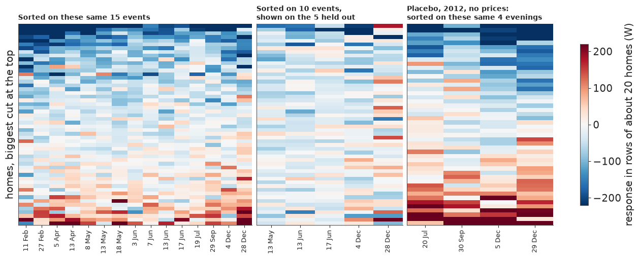
Sorting on the data you display makes a tidy gradient even where nothing is there, as the placebo shows; it looks even stronger than the left panel only because it averages 4 evenings, not 15. The middle panel is what the ranking still knows on unseen evenings: the top rows lean blue, far more faintly. (On 28 December alone the top quartile's gap is about -9 W, se 26: unreadable.)
How noisy is one home? A funnel plot draws each home's mean response against its textbook standard error; with nothing happening, 95% of homes should fall inside.
def funnel_points(table, weights, sigma):
    seen = np.isfinite(table)
    effect_home = np.nansum(table * weights, axis=1) / np.where(seen @ weights > 0, seen @ weights, np.nan)
    se = sigma / np.sqrt(seen @ weights)
    ok = np.isfinite(effect_home) & np.isfinite(se)
    return effect_home[ok], se[ok]


real_x, real_se = funnel_points(r_local, hours_w, watts(table_file["sigma_w"]))
fake_x, fake_se = funnel_points(r_placebo, p_sel["hours"].to_numpy(float), watts(table_file["placebo_sigma_w"]))
fig, axes = plt.subplots(1, 2, figsize=(12.5, 4.8), sharey=True, sharex=True, layout="constrained")
for ax, x, se, title in zip(
    axes, (real_x, fake_x), (real_se, fake_se), ("15 priced evenings, 2013", "4 placebo evenings, 2012: no price")
):
    art = ax.hexbin(
        x, se, gridsize=46, extent=(-800, 800, 0, 240), cmap="Blues", norm=LogNorm(1, 40), mincnt=1, linewidths=0
    )
    grid_se = np.linspace(0, 240, 20)
    ax.plot(1.96 * grid_se, grid_se, color=DUD_C, lw=1.4)
    ax.plot(-1.96 * grid_se, grid_se, color=DUD_C, lw=1.4)
    ax.axvline(0, color=INK, lw=0.7)
    share = (np.abs(x) > 1.96 * se).mean()
    ax.set_title(f"{title}: {share:.0%} outside", fontsize=10.5)
    ax.tick_params(labelsize=10)
    ax.set(xlabel="a home's mean response (W)", xlim=(-600, 600), ylim=(0, 170))
axes[0].set_ylabel("textbook se of that home (W)", fontsize=10.5)
fig.colorbar(art, ax=axes, shrink=0.85, label="homes in a hexagon")
fig.suptitle(
    "With no price at all, three homes in ten look significant: the textbook se of one home is far too small",
    x=0.01,
    ha="left",
    fontsize=11,
)
print(
    f"Homes outside the 95% funnel: priced {(np.abs(real_x) > 1.96 * real_se).mean():.1%}, placebo {(np.abs(fake_x) > 1.96 * fake_se).mean():.1%}"
)
print(
    f"Below the funnel only: priced {(real_x < -1.96 * real_se).mean():.1%}, placebo {(fake_x < -1.96 * fake_se).mean():.1%}"
)
print(
    f"Median textbook se of a home: {np.median(real_se):.0f} W priced, {np.median(fake_se):.0f} W placebo; "
    f"between-home sd {real_x.std():.0f} W, {fake_x.std():.0f} W"
)
matching = np.flatnonzero(frame_r["day"].isin(p_sel["day"]).to_numpy())
print(
    f"The same 4 evenings with prices, 2013: between-home sd {np.nanstd(weighted(r_local, matching, hours_w)):.0f} W, "
    f"so 4 against 15 evenings explains most of 164 W against 80 W"
);
Homes outside the 95% funnel: priced 34.0%, placebo 30.0%
Below the funnel only: priced 27.5%, placebo 16.0%
Median textbook se of a home: 27 W priced, 55 W placebo; between-home sd 80 W, 164 W
The same 4 evenings with prices, 2013: between-home sd 160 W, so 4 against 15 evenings explains most of 164 W against 80 W
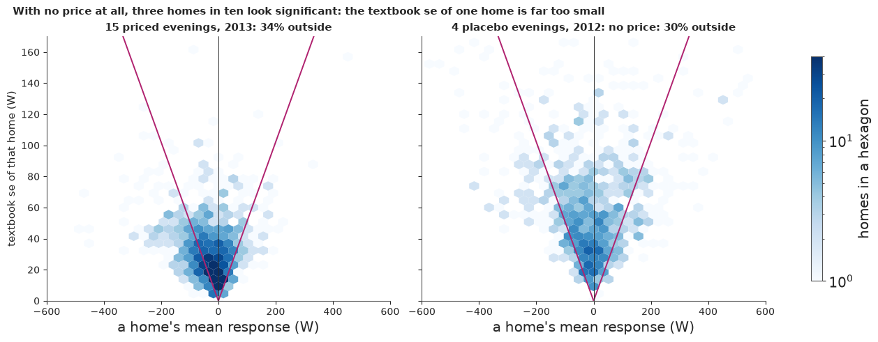
In the placebo only 70% do. Hourly load comes in bursts, so one home's textbook se of 27-55 W is far too small; the real spread between homes is 80 W on 15 evenings and 164 W on 4. Priced homes do lean the right way (27.5% below the funnel against 16% in the placebo), so the response is real, but a list of "best homes" read off one table is mostly a list of noise.
The fix is to rank on some events and score on others. Each evening type has three repeats, so we hold out one repeat of every type in turn. And since an operator has no response history before a trial, we also rank on evening load from July-December 2012, which no price can have touched.
def targeting(baseline="local", top=0.25):
    """Cross-fit on repeats, and rank on pre-trial evening load. Means in W, top against everyone."""
    frame = repeats()
    table = home_tables[baseline][:, frame.index]
    weights, repeat = frame["hours"].to_numpy(float), frame["repeat"].to_numpy()
    folds = []
    for fold in range(3):
        train, test = np.flatnonzero(repeat != fold), np.flatnonzero(repeat == fold)
        score, held = weighted(table, train, weights), weighted(table, test, weights)
        chosen = score <= np.nanquantile(score, top)
        folds.append(
            {
                "held out": ", ".join(pd.Timestamp(d).strftime("%-d %b") for d in frame["day"].to_numpy()[test]),
                "top, same events": np.nanmean(score[chosen]),
                "top, held out": np.nanmean(held[chosen]),
                "all homes, held out": np.nanmean(held),
                "ratio": np.nanmean(held[chosen]) / np.nanmean(held),
                "se of top (homes)": np.nanstd(held[chosen], ddof=1) / np.sqrt(np.isfinite(held[chosen]).sum()),
            }
        )
    folds = pd.DataFrame(folds)
    everyone = weighted(table, np.arange(len(frame)), weights)
    load = watts(table_file["pre_evening_w"])
    big = load >= np.nanquantile(load, 1 - top)
    pre = {
        "top": np.nanmean(everyone[big]),
        "all": np.nanmean(everyone),
        "rest": np.nanmean(everyone[~big & np.isfinite(load)]),
        "se": np.nanstd(everyone[big], ddof=1) / np.sqrt(np.isfinite(everyone[big]).sum()),
        "load_top": np.nanmean(load[big]),
        "load_all": np.nanmean(load),
    }
    return folds, pre


folds, pre = targeting()
print(folds.round(1).to_string(index=False))
same, held, base = (
    folds["top, same events"].mean(),
    folds["top, held out"].mean(),
    folds["all homes, held out"].mean(),
)
print(
    f"\nAll homes {base:.1f} W. Top quartile {same:.1f} W on the same events, {held:.1f} W held out: {held / base:.1f}x the mean, "
    f"against the published 3x. Held-out fold ratios {folds['ratio'].min():.1f} to {folds['ratio'].max():.1f}."
)
print(f"Lost going from same-event to held-out: {1 - held / same:.0%}")
print(f"Same-event ranking on this table: {same / base:.1f}x the mean")
pairs = [
    (weighted(r_local, np.flatnonzero(rep != f), hours_w), weighted(r_local, np.flatnonzero(rep == f), hours_w))
    for f in range(3)
]
print(
    "Correlation of a home's response between ranked and held-out events, by fold:",
    [round(float(np.corrcoef(a[np.isfinite(a + b)], b[np.isfinite(a + b)])[0, 1]), 2) for a, b in pairs],
)
print(
    f"Whole-window baseline: held out {targeting('plan')[0]['top, held out'].mean():.1f} W, all homes {targeting('plan')[0]['all homes, held out'].mean():.1f} W"
)
print(
    f"Ranked on Jul-Dec 2012 evening load, all 15 events: top quartile {pre['top']:.1f} W (se {pre['se']:.1f}), all {pre['all']:.1f} W, the rest {pre['rest']:.1f} W: "
    f"{pre['top'] / pre['all']:.1f}x"
)
print(
    f"As a share of their evening load: top quartile {-pre['top'] / pre['load_top']:.1%} of {pre['load_top']:.0f} W, everyone {-pre['all'] / pre['load_all']:.1%} of {pre['load_all']:.0f} W"
)

load_w = watts(table_file["pre_evening_w"])
is_winter = (frame_r["season"] == "gmt").to_numpy()
is_dud = (frame_r["day"] == DUD_DAY).to_numpy()
big_homes = load_w >= np.nanquantile(load_w, 0.75)


def top_of(table, fold):
    """The top quartile ranked with this fold held out."""
    score = weighted(table, np.flatnonzero(rep != fold), hours_w)
    return score <= np.nanquantile(score, 0.25)


def held_ratio(picked):
    """Top quartile against all homes, on the held-out picked evenings, summed over folds."""
    columns = [(f, c) for f in range(3) for c in np.flatnonzero((rep == f) & picked)]
    tops = {f: top_of(r_local, f) for f, _ in columns}
    return sum(np.nanmean(r_local[tops[f], c]) for f, c in columns) / sum(np.nanmean(r_local[:, c]) for _, c in columns)


def load_ratio(picked):
    values = weighted(r_local, np.flatnonzero(picked), hours_w)
    return np.nanmean(values[big_homes]) / np.nanmean(values)


print(
    "Winter evenings only, top quartile against all:\n"
    + pd.DataFrame(
        {
            name: {"ranked on other events, held out": held_ratio(picked), "ranked on earlier load": load_ratio(picked)}
            for name, picked in (("4 winter", is_winter), ("3 winter", is_winter & ~is_dud))
        }
    )
    .T.round(1)
    .to_string()
)
list_load = [np.nanmean(load_w[top_of(r_local, f)]) for f in range(3)]
print(
    f"The response-ranked list is bigger too: earlier evening load {min(list_load):.0f}-{max(list_load):.0f} W against {pre['load_all']:.0f} W, "
    f"{np.mean([np.nanmean(big_homes[top_of(r_local, f)]) for f in range(3)]):.0%} of it in the top load quartile, "
    f"so {held / base:.1f}x is about {held / base / (np.mean(list_load) / pre['load_all']):.2f}x as a share of load"
)
every_home = weighted(r_local, np.arange(15), hours_w)
boot_rng = np.random.default_rng(RANDOM_SEED + 6)
with stage("Targeting bootstrap"):
    boot = []
    for _ in range(1000):
        pick = boot_rng.integers(0, len(r_local), len(r_local))
        tops = [top_of(r_local[pick], f) for f in range(3)]
        tests = [weighted(r_local[pick], np.flatnonzero(rep == f), hours_w) for f in range(3)]
        loads, values = load_w[pick], every_home[pick]
        big = loads >= np.nanquantile(loads, 0.75)
        boot.append(
            (
                np.mean([np.nanmean(t[s]) for t, s in zip(tests, tops)]) / np.mean([np.nanmean(t) for t in tests]),
                100 * (np.nanmean(values) / np.nanmean(loads) - np.nanmean(values[big]) / np.nanmean(loads[big])),
            )
        )
boot = np.array(boot)
print(
    f"Home bootstrap, 90%: held-out ratio {np.quantile(boot[:, 0], 0.05):.2f} to {np.quantile(boot[:, 0], 0.95):.2f}; "
    f"share of load, top quartile minus everyone {np.quantile(boot[:, 1], 0.05):+.1f} to {np.quantile(boot[:, 1], 0.95):+.1f} points"
)

fig, axes = plt.subplots(1, 2, figsize=(12.5, 4.7), width_ratios=(1.1, 1), layout="constrained")
ax = axes[0]
labels = [
    "Everyone",
    "Top quartile, ranked on\nearlier evening load",
    "Top quartile, ranked on other\nevents, scored held out",
    "Top quartile, ranked and scored\non the same events",
]
values = [-base, -pre["top"], -held, -same]
bars = ax.barh(
    range(4), values, color=[MUTED, SF_C, SF_C, "#e3e3e3"], height=0.62, edgecolor=[MUTED, SF_C, SF_C, MUTED]
)
for yi, v in enumerate(values):
    ax.annotate(f"{v:.0f} W", (v, yi), xytext=(5, 0), textcoords="offset points", va="center", fontsize=10, color=INK)
ax.axvline(-3 * base, color=DUD_C, lw=1.5, ls="--")
ax.annotate(
    "published: 3x the mean",
    (-3 * base, 3.5),
    xytext=(5, 0),
    textcoords="offset points",
    fontsize=9.5,
    color=INK,
    va="center",
)
ax.set_yticks(range(4), labels, fontsize=9.5)
ax.set(xlabel="cut per home on an evening event (W)", xlim=(0, 170), ylim=(-0.5, 3.8))
ax.set_title("What the ranking is worth depends on what it was ranked on", loc="left", fontsize=11)
ax = axes[1]
x_all, y_all = np.concatenate([a for a, _ in pairs]), np.concatenate([b for _, b in pairs])
ok = np.isfinite(x_all) & np.isfinite(y_all)
ax.hexbin(
    x_all[ok],
    y_all[ok],
    gridsize=44,
    extent=(-420, 300, -420, 300),
    cmap="Blues",
    norm=LogNorm(1, 60),
    mincnt=1,
    linewidths=0,
)
edges = np.nanquantile(x_all[ok], np.linspace(0, 1, 11))
centre = [
    (x_all[ok][(x_all[ok] >= a) & (x_all[ok] <= b)].mean(), y_all[ok][(x_all[ok] >= a) & (x_all[ok] <= b)].mean())
    for a, b in zip(edges[:-1], edges[1:])
]
ax.plot([-420, 300], [-420, 300], color=INK, lw=0.8, ls=":", label="a perfect repeat")
ax.plot(*zip(*centre), color=DUD_C, lw=2, marker="o", ms=5, label="mean held-out response, by decile of the ranking")
ax.set(
    xlim=(-420, 300),
    ylim=(-420, 300),
    xlabel="response on the events ranked (W)",
    ylabel="response on the held-out events (W)",
)
ax.legend(loc="upper left", fontsize=9)
ax.set_title("Regression to the mean, home by home", loc="left", fontsize=11);
                             held out  top, same events  top, held out  all homes, held out  ratio  se of top (homes)
  11 Feb, 27 Feb, 5 Apr, 8 May, 7 Jun            -127.5          -88.5                -41.8    2.1               10.9
13 Apr, 18 May, 3 Jun, 19 Jul, 29 Sep            -147.9          -57.2                -23.0    2.5               11.5
13 May, 13 Jun, 17 Jun, 4 Dec, 28 Dec            -148.4          -48.2                -22.5    2.1                9.5

All homes -29.1 W. Top quartile -141.3 W on the same events, -64.6 W held out: 2.2x the mean, against the published 3x. Held-out fold ratios 2.1 to 2.5.
Lost going from same-event to held-out: 54%
Same-event ranking on this table: 4.9x the mean
Correlation of a home's response between ranked and held-out events, by fold: [0.19, 0.14, 0.11]
Whole-window baseline: held out -96.3 W, all homes -41.7 W
Ranked on Jul-Dec 2012 evening load, all 15 events: top quartile -46.4 W (se 7.3), all -29.2 W, the rest -23.5 W: 1.6x
As a share of their evening load: top quartile 4.2% of 1115 W, everyone 5.0% of 582 W
Winter evenings only, top quartile against all:
          ranked on other events, held out  ranked on earlier load
4 winter                               2.2                     1.8
3 winter                               2.1                     1.9
The response-ranked list is bigger too: earlier evening load 733-758 W against 582 W, 40% of it in the top load quartile, so 2.2x is about 1.74x as a share of load
Home bootstrap, 90%: held-out ratio 1.92 to 2.58; share of load, top quartile minus everyone -1.5 to -0.0 points
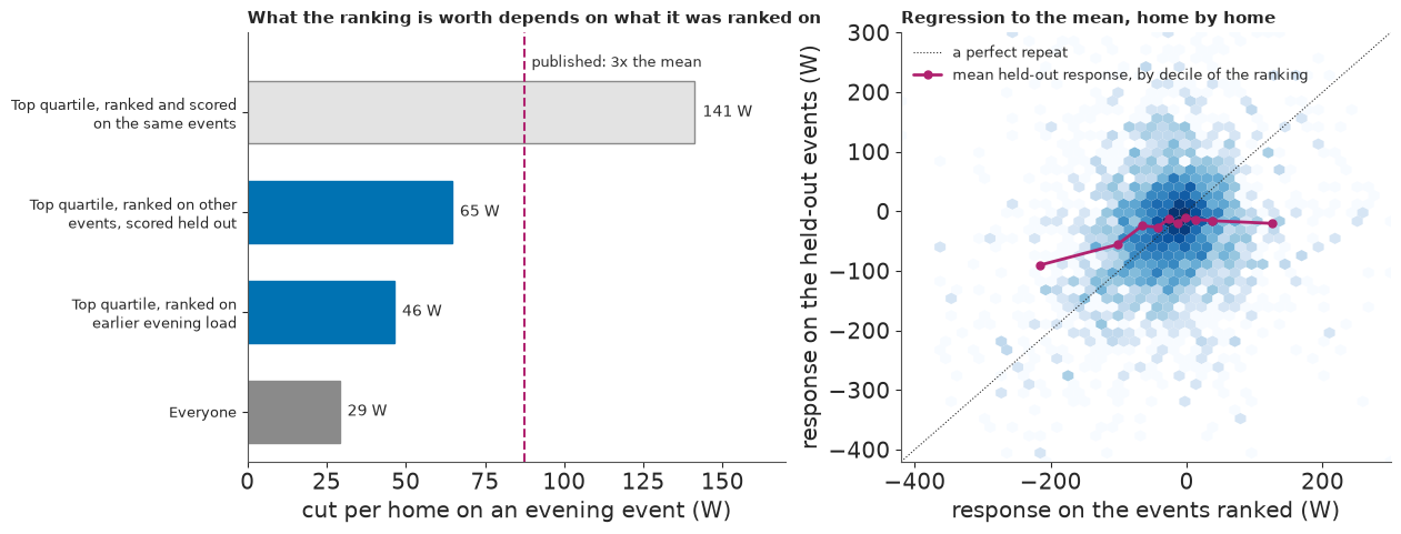
The top quartile reads about -141 W on the events that ranked it and -65 W on events it did not see: 54% of the claimed cut does not repeat. Against all homes on the same held-out events that is about 2.2x the average (folds 2.1-2.5x, home bootstrap 1.9-2.6x). The published 3x is not comparable: same-event ranking here reads 4.9x, so it was not built this way. A home's response on ranked and held-out events correlates at only 0.11-0.19, and the right panel shows the signal sits in the two most extreme deciles. The ranked homes are also bigger (earlier evening load about 730-760 W against 582 W), so as a share of load 2.2x is about 1.7x.
Ranking on earlier load alone gives about 46 W against 29 W, 1.6x (1.8x on winter evenings), with nothing selected on the outcome. But those homes cut 4.2% of their load against 5.0% for everyone: they are bigger, not keener.
These data give no reason to pay for a targeted list, and without cost data we cannot say when it would pay. Response ranking needs a trial first; load ranking mostly picks larger homes. Neither changes section 7, because a smarter list only scales the same four evenings.
9 · What it cost, and what a local trial would need
First the time each stage of this run took, in seconds.
price = pd.Series(PRICE).sort_values(ascending=False)
print(price.round(1).to_string())
print(f"Timed stages {price.sum():.0f} s")
M2, 20 homes                      122.6
M2, compile                        15.4
M4, each evening left out          11.1
M4, peak hours                      8.4
M4, 4 fits                          8.2
M4, own winter spread               7.2
M4, tau_e prior                     3.9
M4, one row borrowing CM            2.2
Targeting bootstrap                 1.0
M1, 200 homes, three baselines      1.0
Fleet curves                        0.1
Timed stages 181 s
The 20 Student-t fits took about two minutes of the 181 timed seconds; the closed-form fleet, which carries every kW figure, took one. Student-t for all 1,088 homes would take about 1.5-2 hours on 2 cores (extrapolated, not run), and where it differed clearly from the mean it was wrong for this purpose. Its value here is the lesson.
The day spread limits everything, so the next cell asks what new winter evenings would buy: the precision of the winter mean, the chance if that mean were known exactly, and how tightly $n$ evenings bound the spread and the share of dead evenings.
spread_low, spread_high = float(np.median(main["tau"])), float(event_means().query("group == 0")["mean"].std())
TRIAL_SIZES = (4, 8, 12, 20, 40)
print(f"How precisely would new winter evenings pin the winter mean? se in W, from day-to-day spread alone:")
print(
    pd.DataFrame({f"day sd {s:.0f} W": {n: s / np.sqrt(n) for n in TRIAL_SIZES} for s in (spread_low, spread_high)})
    .T.round(1)
    .to_string()
)
print("\nP(1 MW at 200,000 offers) if the mean were known exactly and only the day spread remained:")
for spread in (spread_low, float(np.median(own["tau"]))):
    known = {"mu": np.full_like(main["mu"], np.median(own["mu"][:, 0])), "tau": np.full(4000, spread), "sd": main["sd"]}
    print(f"  day sd {spread:.0f} W: {float(chance(known, 0, 200_000)):.2f}")
print("\nWhat a trial could bound, by evenings run:")
print(
    pd.DataFrame(
        {
            "95% upper limit on the day sd, as a multiple of the sd seen": {
                n: np.sqrt((n - 1) / stats.chi2.ppf(0.05, n - 1)) for n in TRIAL_SIZES
            },
            "95% upper limit on the share of dead evenings, if none is seen": {n: 1 - 0.05 ** (1 / n) for n in TRIAL_SIZES},
        }
    )
    .T.round(2)
    .to_string()
)

results = {
    "delivery": delivery_table.round(3).to_dict(),
    "outside_every_headline_range": list(delivery_table.index[-2:]),
    "ways_of_counting": {k: np.round(v, 3).tolist() for k, v in ways.items()},
    "fits": {k: {a: round(float(b), 3) for a, b in v.items()} for k, v in fit_view.items()},
    "targeting": {
        "same_events_w": round(float(same), 1),
        "held_out_w": round(float(held), 1),
        "all_homes_w": round(float(base), 1),
        "pre_trial_top_w": round(float(pre["top"]), 1),
        "pre_trial_all_w": round(float(pre["all"]), 1),
    },
    "student_t_demo": student[["home", "max r_hat", "nu", "divergences"]].round(3).to_dict("list"),
}
store.save_json("notebook_results", results)
print("Stored", "notebook_results", "; store problems:", store.verify() or "none")
How precisely would new winter evenings pin the winter mean? se in W, from day-to-day spread alone:
               4     8    12   20   40
day sd 11 W   5.6   3.9  3.2  2.5  1.8
day sd 30 W  14.9  10.5  8.6  6.7  4.7

P(1 MW at 200,000 offers) if the mean were known exactly and only the day spread remained:
  day sd 11 W: 0.96
  day sd 28 W: 0.74

What a trial could bound, by evenings run:
                                                                  4     8     12    20    40
95% upper limit on the day sd, as a multiple of the sd seen     2.92  1.80  1.55  1.37  1.23
95% upper limit on the share of dead evenings, if none is seen  0.53  0.31  0.22  0.14  0.07
Stored notebook_results ; store problems: none
Today's four evenings pin the winter mean to about 6-15 W from the day spread alone; twelve evenings would give about 3-9 W, and reaching 5 W takes between 5 and 36 evenings, which is the range the evidence leaves open. Pinning the mean is not enough: known exactly, 200,000 offers still reads 0.96 at a day sd of 11 W and 0.74 at 28 W. More evenings help mostly by bounding the spread and the share of dead evenings: twelve clean evenings still allow up to 22% dead, twenty allow 14%.
So the sentence for the planner is this. If one in four of those offered accept, an assumption to replace, about 100,000 offers give an even chance of taking 1 MW, averaged over the priced hours, off a winter evening; 200,000 give somewhere between 0.7 and 0.97, and at face value one evening in four falls short at any scale. Every event after 19 December 2013 showed nothing, for reasons we cannot tell. The advice is not to book the price signal as firm capacity, and to run a local trial of winter evenings first: randomise the evenings, log that each signal was sent, repeat one event type through the winter, price 18:00-20:00, include January and Christmas week on purpose, and measure acceptance. Build any best-responder list from that trial, scored on held-out evenings.
The data are from UK Power Networks' Low Carbon London project, London Datastore, CC BY 4.0, changed as described; no endorsement is implied. Nothing from the UK Data Service release is used.
Summary
- Only the event calendar was randomised. The tariff-minus-flat gap of -69 W on SF evenings was already -18 W before prices existed, so no effect can be read from it; each home was compared with itself instead.
- The meters run on GMT, stamped at the end of the half-hour. A naive wall-clock join silently loses about 12% of the response.
- A closed-form within-home model fits a fleet in seconds and matched the published ranges. The 2012 placebo failed for the placed peak days (+13 W) and was too imprecise for SF High, so only SF evenings carry estimates: a High event cut about 29-42 W per home over the priced hours, the range being the baseline, whose 2013 end was argued for only after the placebo.
- The Student-t likelihood failed quietly:
nuat its floor, stuck chains with no divergences, and a location that saw a quarter of the peak-day cut and an eighth of the SF Low rise. A substation sums means. - Evenings, not homes, limit the answer. Four randomised winter evenings read -68, -59, -33 and -2 W, and every event after 19 December showed nothing, for reasons the data cannot separate. A shared day spread gives a winter mean of -39 W (90% -52 to -26) but misses 28 December in its own check; winter's own spread widens it to -64 to -14 W and leans on its prior.
- How many homes. At an assumed 24% acceptance, 100,000 offers give a 0.4-0.5 chance of 1 MW off a winter evening (0.7-0.9 without 28 December, about 0.2-0.4 without either February evening). At 200,000, counting homes says 1.00 and counting evenings 0.72-0.97. This assumes the four evenings are exchangeable; only three priced the 18:00-20:00 peak, and none fell in January.
- Best responders are oversold by same-event ranking: cross-fitted, the top quartile is worth about 2.2x the average, not 4.9x; ranking on earlier load gives 1.6x, and both lists mostly pick bigger homes.
- Limits. Volunteers, paid and protected against loss, in 2013 London, with no location. We did not test whether the pipeline recovers a known response injected into real noise, so the calibration of these intervals is unchecked.
Try it yourself
- A rate and a target you can defend. Suppose 15% accept and you need 0.5 MW. Run
chance(own, 0, 150_000, acceptance=0.15, target_mw=0.5)and the same withmain. How far apart are the wide and narrow versions? Then size a 2 MW scheme withhomes_needed(own, 2.0, 0.8)and compare it with 2 MW at 50 W a home. - Lose a different evening.
gone = fit_m4(drop=("2013-02-11",)), thenfloat(chance(gone, 0, 100_000))andnp.median(gone["mu"][:, 0]). If one evening can swing the answer each way, what does that say about four? - A smaller elite. Run
elite, _ = targeting(top=0.10), thenelite["top, held out"].mean() / elite["all homes, held out"].mean(). Does the ratio rise as the list shrinks, and how many homes does that leave to carry a megawatt?