The brief
The operations team of a bike-sharing scheme plans two things a day ahead: how many vans and staff to put on rebalancing (moving bikes from full docks to empty ones), and how many bikes to have in service. Both scale with the number of rentals they must be able to serve tomorrow. Plan too low and customers find empty docks; plan too high and vans and people stand idle.
They have a weather forecast for tomorrow and two years of history. What they ask for:
"Give us tomorrow's demand with a range we can trust. If you say 90%, we want to be inside it nine days out of ten. And tell us how much capacity to plan so that we can cover demand on 95% of days."
From conversations with the team you know that a typical day sees a few thousand rentals, that a busy summer day can reach eight thousand, and that the system is growing fast.
A point forecast is the easy half of this. The brief is about the spread: a predictive distribution whose stated probabilities can be taken at face value. Sampler diagnostics will not tell you whether you have one.
How this notebook works
- Each task states what to deliver, not how. Write your code in the
YOUR CODE HEREcells. - Stuck?
h.hint("task2")reveals hints one level at a time: nudge → approach → code skeleton. Try to get by on nudges. h.check("task2", coverage90=...)compares your numbers with the reference solution.- A full worked solution lives in
notebooks/solutions/. Open it only when you are done (or truly stuck).
import arviz as az
import matplotlib.pyplot as plt
import numpy as np
import pandas as pd
import pymc as pm

from pymc_challenges import Hints, data

RANDOM_SEED = 2012
rng = np.random.default_rng(RANDOM_SEED)
az.style.use("arviz-variat")

h = Hints("C03")
h.tasks()
C03 - Bike sharing: demand forecasts that admit what they do not know
task0- Decode, split, look (2 hints, 2 check(s))task1- The textbook model for counts (3 hints, 1 check(s))task2- Fix what Task 1 revealed (3 hints, 3 check(s))task3- Too hot to cycle (3 hints, 2 check(s))task4- Calendar, weather situation, growth - and a scoreboard (3 hints, 2 check(s))task5- The days the model cannot believe (3 hints, 2 check(s))task6- Open the hold-out (3 hints, 3 check(s))task7- How much capacity? (3 hints, 3 check(s))
The data
One row per day, 1 January 2011 to 31 December 2012. cnt is the total number of rentals
(casual + registered). Calendar columns: yr (0 = 2011, 1 = 2012), mnth, weekday
(an integer - find out which day is 0), holiday, workingday (neither weekend nor
holiday). weathersit is the day's weather situation: 1 = clear or partly cloudy,
2 = mist or overcast, 3 = light rain or snow, thunderstorm.
The UCI file stores the continuous weather variables normalised - each was divided by a constant so that it lies between 0 and 1:
| column | meaning | divided by |
|---|---|---|
temp |
mean temperature, °C | 41 |
atemp |
"feels-like" temperature, °C | 50 |
hum |
relative humidity, % | 100 |
windspeed |
wind speed, km/h | 67 |
Nobody on the operations team thinks in units of "0.34 of 41 °C".
data.describe("bike_day")
raw = data.load("bike_day")
raw.head()
bike_day: Daily rental counts 2011-2012 with weather and calendar covariates.
  source: Fanaee-T & Gama (2013), Capital Bikeshare (Washington DC), UCI ML Repository.
  url:    https://archive.ics.uci.edu/static/public/275/bike+sharing+dataset.zip
| instant | dteday | season | yr | mnth | holiday | weekday | workingday | weathersit | temp | atemp | hum | windspeed | casual | registered | cnt | |
|---|---|---|---|---|---|---|---|---|---|---|---|---|---|---|---|---|
| 0 | 1 | 2011-01-01 | 1 | 0 | 1 | 0 | 6 | 0 | 2 | 0.344167 | 0.363625 | 0.805833 | 0.160446 | 331 | 654 | 985 |
| 1 | 2 | 2011-01-02 | 1 | 0 | 1 | 0 | 0 | 0 | 2 | 0.363478 | 0.353739 | 0.696087 | 0.248539 | 131 | 670 | 801 |
| 2 | 3 | 2011-01-03 | 1 | 0 | 1 | 0 | 1 | 1 | 1 | 0.196364 | 0.189405 | 0.437273 | 0.248309 | 120 | 1229 | 1349 |
| 3 | 4 | 2011-01-04 | 1 | 0 | 1 | 0 | 2 | 1 | 1 | 0.200000 | 0.212122 | 0.590435 | 0.160296 | 108 | 1454 | 1562 |
| 4 | 5 | 2011-01-05 | 1 | 0 | 1 | 0 | 3 | 1 | 1 | 0.226957 | 0.229270 | 0.436957 | 0.186900 | 82 | 1518 | 1600 |
The final eight weeks (56 days, from 6 November 2012) are the hold-out. They stay locked away until Task 6: no plots, no fitting, no peeking.
HOLDOUT_START = pd.Timestamp("2012-11-06")
Task 0 · Decode, split, look
Deliver
- A data frame with the weather in physical units (°C, %, km/h) and readable labels for weekday and weather situation. Verify the weekday coding rather than guessing it.
train(beforeHOLDOUT_START) andtest(the rest).- Plots of the training data that show what a demand model will have to reproduce: the
series over time, demand against temperature, demand by weather situation and by weekday.
Write down the three or four features you consider essential. Do you need both
tempandatemp?
WEEKDAYS = ["Sun", "Mon", "Tue", "Wed", "Thu", "Fri", "Sat"]
WEATHER = ["clear", "mist", "wet"]

# which day is weekday 0? ask the dates instead of guessing
print(pd.crosstab(raw.dteday.dt.day_name(), raw.weekday).idxmax().to_dict())


def prepare(df):
    return df.assign(
        temp_c=df.temp * 41,
        hum_pct=df.hum * 100,
        wind_kmh=df.windspeed * 67,
        t=(df.dteday - pd.Timestamp("2011-01-01")).dt.days / 365.25,  # time in years
        weekday_name=pd.Categorical.from_codes(df.weekday, WEEKDAYS),
        weather=pd.Categorical.from_codes(df.weathersit - 1, WEATHER),
    )


bikes = prepare(raw)
train = bikes[bikes.dteday < HOLDOUT_START].copy()
test = bikes[bikes.dteday >= HOLDOUT_START].copy()
print(f"train: {len(train)} days, test: {len(test)} days")
print(f"correlation of temp and atemp: {bikes.temp_c.corr(bikes.atemp):.3f}")
bikes[["temp_c", "hum_pct", "wind_kmh", "cnt"]].describe().round(1)
{0: 'Sunday', 1: 'Monday', 2: 'Tuesday', 3: 'Wednesday', 4: 'Thursday', 5: 'Friday', 6: 'Saturday'}
train: 675 days, test: 56 days
correlation of temp and atemp: 0.992| temp_c | hum_pct | wind_kmh | cnt | |
|---|---|---|---|---|
| count | 731.0 | 731.0 | 731.0 | 731.0 |
| mean | 20.3 | 62.8 | 12.8 | 4504.3 |
| std | 7.5 | 14.2 | 5.2 | 1937.2 |
| min | 2.4 | 0.0 | 1.5 | 22.0 |
| 25% | 13.8 | 52.0 | 9.0 | 3152.0 |
| 50% | 20.4 | 62.7 | 12.1 | 4548.0 |
| 75% | 26.9 | 73.0 | 15.6 | 5956.0 |
| max | 35.3 | 97.2 | 34.0 | 8714.0 |
assert h.check("task0", mean_temp_c=bikes.temp_c.mean(), max_wind_kmh=bikes.wind_kmh.max())
- PASS
mean_temp_c= 20.31 is consistent with the reference solution. - PASS
max_wind_kmh= 34 is consistent with the reference solution.
fig, axes = plt.subplots(2, 2, figsize=(12, 7.5))
ax = axes[0, 0]
for i, w in enumerate(WEATHER):
    d = train[train.weather == w]
    ax.scatter(d.dteday, d.cnt, s=9, color=f"C{i}", label=w)
ax.set(ylabel="rentals per day", title="Training period")
ax.legend(loc="upper left")
ax.tick_params(axis="x", rotation=30)

ax = axes[0, 1]
for yr, d in train.groupby("yr"):
    ax.scatter(d.temp_c, d.cnt, s=9, color=f"C{yr + 3}", label=str(2011 + yr), alpha=0.8)
ax.set(xlabel="temperature (°C)", ylabel="rentals per day")
ax.legend()

for ax, col in zip(axes[1], ["weather", "weekday_name"]):
    groups = [d.cnt.values for _, d in train.groupby(col, observed=True)]
    ax.boxplot(groups, tick_labels=list(train[col].cat.categories))
    ax.set(ylabel="rentals per day", xlabel=col.replace("_name", ""));
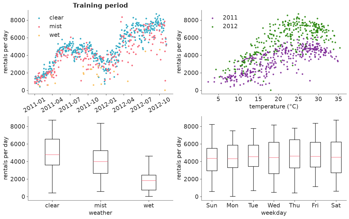
What a demand model has to reproduce:
- Growth. 2012 sits well above 2011 at every temperature; the two years form two separate clouds in the temperature plot.
- Temperature, but not linearly. Demand rises steeply from 5 to about 25 °C, flattens, and falls on the hottest days.
- Weather situation. The median wet day has well under half the rentals of the median clear day. Weekday differences in the total are small by comparison.
- A lot of scatter, and a few extreme days. At any given temperature, days differ by thousands of rentals, and a handful of days sit far below everything around them - one at the end of October 2012 is practically zero.
temp and atemp are correlated at 0.99. Using both would add nothing but a ridge in the
posterior; we keep temp.
Task 1 · The textbook model for counts
Rentals are counts, so start where every textbook starts: a Poisson regression with a log link. Use the weather only - temperature, humidity and wind speed, each entering linearly on the log scale.
Deliver
- Priors you can defend, shown with a prior predictive check on the scale the operations team thinks in: rentals per day.
- A fit with clean sampler diagnostics. Look at how precisely the model claims to know its coefficients.
- A verdict: is this model's predictive distribution fit for the brief? Back it with at least one graphical posterior predictive check that could embarrass the model, and one number: the share of training days that fall inside the model's central 90% predictive interval.
Solution
Priors. With a log link, coefficients act multiplicatively, so we think in factors. The
team told us a typical day sees a few thousand rentals: Normal(log(4000), 1) for the
intercept puts one prior standard deviation at a factor of e ≈ 2.7 either way. The
predictors are standardised (with training means and standard deviations, stored so that
future days get the same transformation), and Normal(0, 0.5) says that one standard
deviation of temperature most likely changes demand by less than a factor of
e^0.5 ≈ 1.65, and almost certainly by less than e^1.5 ≈ 4.5.
WEATHER_COLS = ["temp_c", "hum_pct", "wind_kmh"]
SCALE = train[WEATHER_COLS].agg(["mean", "std"])  # fixed once, so new days get the same units


def standardise(df):
    return (df[WEATHER_COLS] - SCALE.loc["mean"]) / SCALE.loc["std"]


Z = standardise(train)
coords = {"predictor": WEATHER_COLS, "day": train.dteday.values}

with pm.Model(coords=coords) as poisson_model:
    intercept = pm.Normal("intercept", np.log(4000), 1)
    beta = pm.Normal("beta", 0, 0.5, dims="predictor")
    mu = pm.math.exp(intercept + pm.math.dot(Z.values, beta))
    pm.Poisson("cnt", mu, observed=train.cnt.values, dims="day")
    poisson_prior = pm.sample_prior_predictive(1000, random_seed=RANDOM_SEED)

prior_cnt = poisson_prior.prior_predictive["cnt"].values.ravel()
print("prior predictive rentals per day, quantiles:")
print(pd.Series(prior_cnt).quantile([0.01, 0.25, 0.5, 0.75, 0.99]).round(0).to_string())
prior predictive rentals per day, quantiles:
0.01       168.0
0.25      1718.0
0.50      4051.0
0.75      9828.0
0.99    102428.0
Half of the prior predictive mass is between about 1,700 and 9,800 rentals a day, and 98% of
it between roughly 170 and 100,000. Generous, but every one of those numbers is a bike-share
system that could exist somewhere. For contrast, take a "vague" Normal(0, 10) intercept:
one prior standard deviation above zero is e^10 ≈ 22,000 rentals a day, two are
e^20 ≈ 500 million. After an exp, vague priors are absurd priors.
def fit(model, **kwargs):
    """Sample, then add posterior predictive draws and the pointwise log-likelihood (for LOO)."""
    with model:
        idata = pm.sample(random_seed=RANDOM_SEED, **kwargs)
        pm.sample_posterior_predictive(idata, extend_inferencedata=True, random_seed=RANDOM_SEED)
        pm.compute_log_likelihood(idata, progressbar=False)
    summary = az.summary(idata, round_to="none")
    print(f"divergences: {int(idata.sample_stats['diverging'].sum())}   "
          f"max r_hat: {summary.r_hat.max():.3f}   min ess_bulk: {summary.ess_bulk.min():.0f}")
    return idata


poisson_idata = fit(poisson_model)
az.summary(poisson_idata, round_to=4)
divergences: 0 max r_hat: 1.002 min ess_bulk: 4639
| mean | sd | eti89_lb | eti89_ub | ess_bulk | ess_tail | r_hat | mcse_mean | mcse_sd | |
|---|---|---|---|---|---|---|---|---|---|
| intercept | 8.3662 | 0.0006 | 8.3653 | 8.3672 | 5605.1101 | 3393.1924 | 1.0011 | 0.0 | 0.0 |
| beta[temp_c] | 0.2900 | 0.0006 | 0.2890 | 0.2909 | 4639.0636 | 3473.4294 | 1.0010 | 0.0 | 0.0 |
| beta[hum_pct] | -0.0965 | 0.0006 | -0.0975 | -0.0956 | 5929.1468 | 3507.2947 | 0.9998 | 0.0 | 0.0 |
| beta[wind_kmh] | -0.0760 | 0.0006 | -0.0771 | -0.0750 | 5033.8099 | 3294.7740 | 1.0019 | 0.0 | 0.0 |
def interval(pp, prob):
    """Central predictive interval per day from predictive draws with chain and draw dimensions."""
    q = pp.quantile([(1 - prob) / 2, (1 + prob) / 2], dim=("chain", "draw"))
    return q.isel(quantile=0).values, q.isel(quantile=1).values


def coverage(pp, y, prob=0.9):
    lo, hi = interval(pp, prob)
    return float(np.mean((y >= lo) & (y <= hi)))


def plot_band(dates, pp, y, ax, title):
    lo, hi = interval(pp, 0.9)
    inside = (y >= lo) & (y <= hi)
    ax.fill_between(dates, lo, hi, color="C0", alpha=0.5, lw=0, label="90% predictive interval")
    ax.scatter(dates[inside], y[inside], s=8, color="k", label="observed, inside")
    ax.scatter(dates[~inside], y[~inside], s=8, color="C3", label="observed, outside")
    ax.set(ylabel="rentals per day", title=f"{title}: {inside.mean():.0%} of days inside")
    ax.legend(ncols=3, loc="upper left")


fig, ax = plt.subplots(figsize=(12, 3.8))
plot_band(train.dteday.values, poisson_idata.posterior_predictive["cnt"], train.cnt.values, ax, "Poisson")
az.plot_ppc_pit(poisson_idata);
def dispersion(idata, y, n_params):
    """Pearson statistic / degrees of freedom: about 1 if the variance really equals the mean."""
    mu_hat = idata.posterior_predictive["cnt"].mean(("chain", "draw")).values
    return float(np.sum((y - mu_hat) ** 2 / mu_hat) / (len(y) - n_params))


poisson_cov = coverage(poisson_idata.posterior_predictive["cnt"], train.cnt.values)
poisson_disp = dispersion(poisson_idata, train.cnt.values, n_params=4)
print(f"coverage of the 90% interval: {poisson_cov:.1%}")
print(f"Pearson dispersion statistic: {poisson_disp:.0f}")
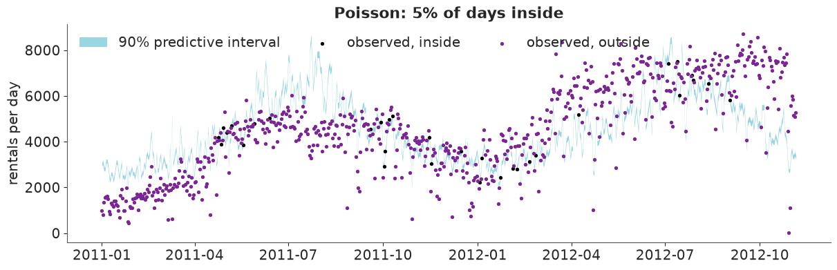
coverage of the 90% interval: 4.7%
Pearson dispersion statistic: 494
assert h.check("task1", coverage90=poisson_cov)
- PASS
coverage90= 0.04741 is consistent with the reference solution.
The sampler is fine. The model is not. r_hat of 1.00, thousands of effective draws, no
divergences - and a posterior standard deviation of 0.0006 on every coefficient: the model
claims to know the temperature effect to three decimal places.
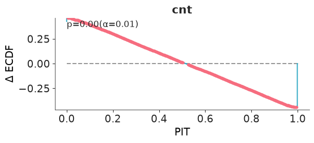
Now the predictive checks. The 90% predictive band is a thin ribbon and only 5% of days fall inside it, where 90% should. The PIT check says the same thing. For each day, the PIT value is the share of predictive draws below the observed count; if the predictive distributions were right these values would be uniform and the Δ-ECDF curve would hug zero. Instead it runs in a straight line from about +0.45 to -0.45 (ArviZ highlights the points that break uniformity - here all of them - and prints the p-value of a uniformity test: 0.00). Almost half of all days sit in the extreme lower tail of their own predictive distribution and almost half in the extreme upper tail.
Why: a Poisson distribution has one parameter, so fixing the mean fixes the spread. With a mean of 4,500 the standard deviation is √4500 ≈ 67 and a 90% interval is about ±110 rentals. Real days differ from the model's expectation by thousands. The Pearson statistic $\sum (y-\mu)^2/\mu \,/\, (n-p)$ would be about 1 if variance equalled mean; here it is 494. (The band plot also shows that the mean is poor - the model knows nothing about growth - and that inflates the statistic. But no set of predictors gets it anywhere near 1: keep an eye on the dispersion parameter as the mean model improves.)
A marginal density overlay (az.plot_ppc_dist) is a weak check here: most of the spread of
daily counts comes from the seasons, which the Poisson model reproduces through its mean.
What the brief needs is the conditional distribution - given tomorrow's weather, how
wide? - and that is what coverage and PIT test. (az.plot_ppc_rootogram is designed for
this question too, but for small counts; with counts in the thousands it takes minutes and
shows nothing.)
Task 2 · Fix what Task 1 revealed
Your verdict should have been damning, and "the sampler is fine" is no defence.
Deliver
- The diagnosis in one sentence: which assumption of the Task 1 model do the data violate, and by roughly what factor? (A number, please.)
- A repaired model that changes only what the diagnosis demands - same predictors, same priors for the coefficients. Explain what its new parameter means in words the operations team would understand.
- The same checks as in Task 1, now passed (or not?).
- Put the posterior standard deviations of the coefficients from both models side by side. What happened, and what would it have cost someone who believed the first model?
Solution
Diagnosis: the Poisson assumption variance = mean fails by a factor of about 500 (overdispersion). Rentals are not independent events at a fixed rate: one rainy hour, a festival or a Metro delay moves thousands of trips together.
Repair: the negative binomial keeps the mean $\mu$ and adds one parameter:
$\text{Var}(y) = \mu + \mu^2/\alpha$. For counts in the thousands the first term is
negligible, so the standard deviation is $\mu/\sqrt{\alpha}$: demand scatters around its
expectation by a constant percentage. That percentage, $cv = 1/\sqrt{\alpha}$, is something the
operations team can relate to, so we put the prior on it directly - HalfNormal(0.5): day-
to-day scatter of tens of percent is plausible, several hundred percent is not - and derive
$\alpha$ from it.
with pm.Model(coords=coords) as negbin_model:
    intercept = pm.Normal("intercept", np.log(4000), 1)
    beta = pm.Normal("beta", 0, 0.5, dims="predictor")
    cv = pm.HalfNormal("cv", 0.5)  # day-to-day coefficient of variation beyond Poisson noise
    alpha = pm.Deterministic("alpha", cv**-2)
    mu = pm.math.exp(intercept + pm.math.dot(Z.values, beta))
    pm.NegativeBinomial("cnt", mu=mu, alpha=alpha, observed=train.cnt.values, dims="day")

negbin_idata = fit(negbin_model)
az.summary(negbin_idata, round_to=3)
divergences: 0 max r_hat: 1.002 min ess_bulk: 4890
| mean | sd | eti89_lb | eti89_ub | ess_bulk | ess_tail | r_hat | mcse_mean | mcse_sd | |
|---|---|---|---|---|---|---|---|---|---|
| intercept | 8.356 | 0.014 | 8.333 | 8.379 | 6710.342 | 3518.893 | 1.000 | 0.000 | 0.000 |
| beta[temp_c] | 0.357 | 0.016 | 0.331 | 0.381 | 5579.699 | 2928.226 | 1.002 | 0.000 | 0.000 |
| beta[hum_pct] | -0.127 | 0.016 | -0.152 | -0.101 | 5753.962 | 3553.410 | 1.001 | 0.000 | 0.000 |
| beta[wind_kmh] | -0.086 | 0.015 | -0.110 | -0.063 | 4890.181 | 3374.378 | 1.000 | 0.000 | 0.000 |
| cv | 0.376 | 0.010 | 0.361 | 0.392 | 5963.780 | 3564.517 | 1.001 | 0.000 | 0.000 |
| alpha | 7.089 | 0.373 | 6.503 | 7.688 | 5963.780 | 3564.517 | 1.001 | 0.005 | 0.005 |
fig, ax = plt.subplots(figsize=(12, 3.8))
plot_band(train.dteday.values, negbin_idata.posterior_predictive["cnt"], train.cnt.values, ax, "Negative binomial")
az.plot_ppc_pit(negbin_idata);
negbin_cov = coverage(negbin_idata.posterior_predictive["cnt"], train.cnt.values)
print(f"coverage of the 90% interval: {negbin_cov:.1%}")

sd = pd.DataFrame({
    "Poisson sd": az.summary(poisson_idata, var_names=["intercept", "beta"], round_to="none")["sd"],
    "NegBin sd": az.summary(negbin_idata, var_names=["intercept", "beta"], round_to="none")["sd"],
})
sd["ratio"] = sd["NegBin sd"] / sd["Poisson sd"]
sd.round(4)
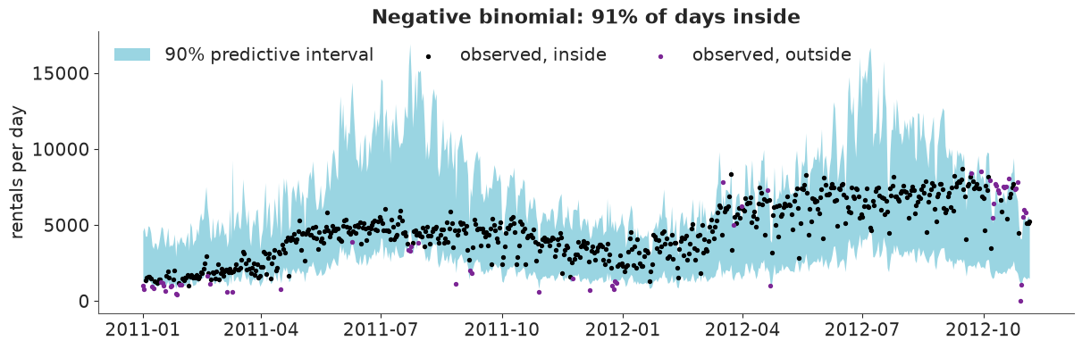
coverage of the 90% interval: 91.1%
| Poisson sd | NegBin sd | ratio | |
|---|---|---|---|
| intercept | 0.0006 | 0.0145 | 23.8307 |
| beta[temp_c] | 0.0006 | 0.0160 | 26.1570 |
| beta[hum_pct] | 0.0006 | 0.0160 | 26.3387 |
| beta[wind_kmh] | 0.0006 | 0.0151 | 23.4213 |
assert h.check(
    "task2",
    dispersion=poisson_disp,
    coverage90=negbin_cov,
    alpha=negbin_idata.posterior["alpha"].mean(),
)
- PASS
dispersion= 494.4 is consistent with the reference solution. - PASS
coverage90= 0.9111 is consistent with the reference solution. - PASS
alpha= 7.089 is consistent with the reference solution.
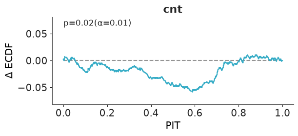
- Coverage: 91%, and the PIT curve now stays within 0.06 of zero instead of ±0.45 (mind
the axis). The uniformity test gives p = 0.02: no longer a disaster, not yet a clean bill
of health.
cvis 0.38: knowing temperature, humidity and wind still leaves demand uncertain by ±38% (one standard deviation). - Honest is not the same as useful. Look at the band: on a summer day it runs from 3,000 to 15,000 rentals. Nobody can plan with that. And the misses are not scattered at random: they bunch below the band in early 2011 and above it in autumn 2012. Calibration on average is the minimum requirement; sharpness has to come from a better model for the mean, which is the business of the next two tasks.
- The coefficients' standard deviations grew by a factor of 23 to 26 - about √494 ≈ 22, which is what quasi-likelihood theory predicts for this much overdispersion. The Poisson model treated each of three million rentals as an independent piece of evidence; in truth there are 675 noisy days. Anyone who believed it would have declared every conceivable predictor "significant" and would have planned capacity with a margin of ±110 rentals. The estimates themselves moved too (temperature from 0.29 to 0.36): the Poisson fit is dominated by the busiest days.
Task 3 · Too hot to cycle
A straight line on the log scale says every extra degree multiplies demand by the same factor, for ever. Washington summers disagree.
Deliver
- Evidence from the Task 2 model that the linear temperature effect is wrong (a residual plot will do).
- A model in which temperature enters through a smooth function instead. Everything else stays as in Task 2.
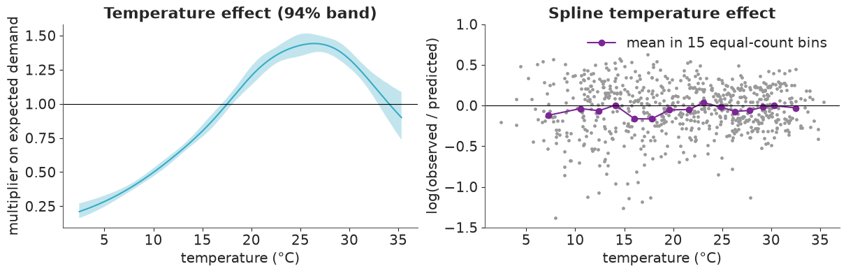
- A plot of the estimated temperature effect as a multiplier on expected demand, with a credible band, across the observed temperature range.
- Two numbers with uncertainty: the temperature at which demand peaks, and how much lower (in %) expected demand is at 35 °C than at the peak.
def log_residual(idata, y):
    return np.log(y) - np.log(idata.posterior_predictive["cnt"].mean(("chain", "draw")).values)


def plot_residual_vs_temp(idata, df, ax, title):
    res = pd.DataFrame({"temp_c": df.temp_c.values, "res": log_residual(idata, df.cnt.values)})
    binned = res.groupby(pd.qcut(res.temp_c, 15), observed=True).mean()
    ax.scatter(res.temp_c, res.res, s=6, color="0.6")
    ax.plot(binned.temp_c, binned.res, "o-", color="C3", label="mean in 15 equal-count bins")
    ax.axhline(0, color="k", lw=0.8)
    ax.set(xlabel="temperature (°C)", ylabel="log(observed / predicted)", title=title, ylim=(-1.5, 1))
    ax.legend()


fig, ax = plt.subplots(figsize=(7, 3.8))
plot_residual_vs_temp(negbin_idata, train, ax, "Linear temperature effect")
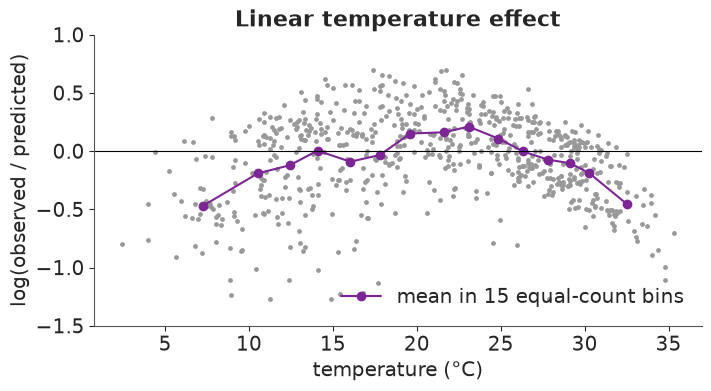
An inverted U. Around 20-25 °C the model predicts too little (binned residuals of +0.15 to +0.2 on the log scale); at both ends far too much: about -0.45 for the coldest and for the hottest bin, which means observed demand is only e^-0.45 ≈ 64% of the prediction. A straight line cannot rise steeply, flatten and come down again.
The fix: a regression spline. patsy turns the temperature column into six smooth
basis functions (a natural cubic spline with knots at quantiles of the training data). The
model stays a GLM - six coefficients instead of one - and the curve is
$f(\text{temp}) = \sum_k w_k B_k(\text{temp})$. Two details matter later: the basis is
centred, so the intercept keeps its meaning as the log of typical demand; and we keep the
design_info, so that new temperatures are expanded with the same knots.
From here on one function builds every model, with all inputs registered as pm.Data and the
likelihood given shape=mu.shape, because we are going to forecast with it.
from patsy import build_design_matrices, dmatrix

# natural cubic regression spline, 6 basis functions, knots at quantiles of the training temperatures;
# "center" removes the constant so the spline does not compete with the intercept
TEMP_SPLINE = dmatrix("cr(temp_c, df=6, constraints='center') - 1", train)


def spline_basis(df):
    """Evaluate the SAME basis (same knots, same centring) for new temperatures."""
    return np.asarray(build_design_matrices([TEMP_SPLINE.design_info], df)[0])


def features(df):
    z = standardise(df)
    return {
        "B": spline_basis(df),
        "hum": z.hum_pct.values,
        "wind": z.wind_kmh.values,
        "weekday_idx": df.weekday.values,
        "weather_idx": df.weathersit.values - 1,
        "holiday": df.holiday.values.astype(float),
        "year2012": df.yr.values - 0.5,
        "t": df.t.values - 1.0,  # years, centred on 1 January 2012
    }


def demand_model(df, calendar=False, trend=None):
    """Negative-binomial demand model. All inputs are pm.Data so that we can forecast later."""
    f = features(df)
    coords = {"knot": np.arange(f["B"].shape[1]), "weekday": WEEKDAYS, "weather": WEATHER, "day": df.dteday.values}
    with pm.Model(coords=coords) as model:
        X = {k: pm.Data(k, v, dims=("day", "knot") if k == "B" else "day") for k, v in f.items()}

        intercept = pm.Normal("intercept", np.log(4000), 1)
        w_temp = pm.Normal("w_temp", 0, 1, dims="knot")
        b_hum = pm.Normal("b_hum", 0, 0.5)
        b_wind = pm.Normal("b_wind", 0, 0.5)
        eta = intercept + pm.math.dot(X["B"], w_temp) + b_hum * X["hum"] + b_wind * X["wind"]

        if calendar:
            weekday_eff = pm.ZeroSumNormal("weekday_eff", 0.3, dims="weekday")
            weather_eff = pm.ZeroSumNormal("weather_eff", 0.5, dims="weather")
            b_holiday = pm.Normal("b_holiday", 0, 0.5)
            eta = eta + weekday_eff[X["weekday_idx"]] + weather_eff[X["weather_idx"]] + b_holiday * X["holiday"]
        if trend is not None:
            growth = pm.Normal("growth", 0, 1)  # change in log demand per year
            eta = eta + growth * (X["year2012"] if trend == "step" else X["t"])

        cv = pm.HalfNormal("cv", 0.5)
        alpha = pm.Deterministic("alpha", cv**-2)
        mu = pm.math.exp(eta)
        pm.NegativeBinomial("cnt", mu=mu, alpha=alpha, observed=df.cnt.values, dims="day", shape=mu.shape)
    return model


spline_model = demand_model(train)
spline_idata = fit(spline_model)
az.summary(spline_idata, var_names=["~alpha"], round_to=3)
divergences: 0 max r_hat: 1.006 min ess_bulk: 755
| mean | sd | eti89_lb | eti89_ub | ess_bulk | ess_tail | r_hat | mcse_mean | mcse_sd | |
|---|---|---|---|---|---|---|---|---|---|
| intercept | 8.337 | 0.013 | 8.317 | 8.357 | 6528.831 | 3022.096 | 1.003 | 0.000 | 0.000 |
| w_temp[0] | 0.223 | 0.083 | 0.090 | 0.352 | 754.525 | 1383.914 | 1.006 | 0.003 | 0.002 |
| w_temp[1] | 0.271 | 0.041 | 0.204 | 0.338 | 1328.949 | 1904.051 | 1.003 | 0.001 | 0.001 |
| w_temp[2] | 0.819 | 0.065 | 0.712 | 0.923 | 930.632 | 1653.224 | 1.005 | 0.002 | 0.001 |
| w_temp[3] | 0.914 | 0.057 | 0.823 | 1.005 | 906.405 | 1497.019 | 1.005 | 0.002 | 0.001 |
| w_temp[4] | 1.188 | 0.081 | 1.057 | 1.317 | 856.600 | 1389.687 | 1.006 | 0.003 | 0.001 |
| w_temp[5] | 0.004 | 0.104 | -0.162 | 0.170 | 5059.266 | 2917.481 | 1.000 | 0.001 | 0.002 |
| b_hum | -0.179 | 0.014 | -0.202 | -0.156 | 5419.356 | 3469.810 | 1.000 | 0.000 | 0.000 |
| b_wind | -0.107 | 0.013 | -0.129 | -0.086 | 5964.008 | 2890.250 | 1.002 | 0.000 | 0.000 |
| cv | 0.324 | 0.009 | 0.310 | 0.338 | 6815.385 | 3115.146 | 1.002 | 0.000 | 0.000 |
temp_grid = pd.DataFrame({"temp_c": np.linspace(train.temp_c.min(), train.temp_c.max(), 200)})
B_grid = spline_basis(temp_grid)


def temperature_curves(idata):
    """Posterior draws of the spline f(temp) on the grid: array (draws, grid)."""
    w = az.extract(idata, var_names="w_temp").transpose("sample", "knot").values
    return w @ B_grid.T


f_temp = temperature_curves(spline_idata)
peak_temp = temp_grid.temp_c.values[f_temp.argmax(axis=1)]
i35 = np.abs(temp_grid.temp_c.values - 35).argmin()
drop35 = 100 * (1 - np.exp(f_temp[:, i35] - f_temp.max(axis=1)))

fig, axes = plt.subplots(1, 2, figsize=(12, 3.8))
lo, hi = np.quantile(np.exp(f_temp), [0.03, 0.97], axis=0)
axes[0].fill_between(temp_grid.temp_c, lo, hi, alpha=0.3)
axes[0].plot(temp_grid.temp_c, np.exp(f_temp).mean(axis=0))
axes[0].axhline(1, color="k", lw=0.8)
axes[0].set(xlabel="temperature (°C)", ylabel="multiplier on expected demand", title="Temperature effect (94% band)")
plot_residual_vs_temp(spline_idata, train, axes[1], "Spline temperature effect")

print(f"training days hotter than 33 °C: {(train.temp_c > 33).sum()}")
print(f"demand peaks at {peak_temp.mean():.1f} °C, 94% interval {np.quantile(peak_temp, [0.03, 0.97]).round(1)}")
print(f"at 35 °C demand is {drop35.mean():.0f}% below the peak, 94% interval {np.quantile(drop35, [0.03, 0.97]).round(0)}")
training days hotter than 33 °C: 15
demand peaks at 26.4 °C, 94% interval [24.6 28.2]
at 35 °C demand is 36% below the peak, 94% interval [23. 48.]
assert h.check("task3", peak_temp_c=peak_temp.mean(), drop_at_35_pct=drop35.mean())
- PASS
peak_temp_c= 26.41 is consistent with the reference solution. - PASS
drop_at_35_pct= 36.25 is consistent with the reference solution.
The binned residuals are flat now, and the curve is what a cyclist would draw. Relative to an average day, the coldest days (2-3 °C) have about a fifth of the demand; demand peaks at 26 °C (94% interval 24.6 to 28.2) at about 1.45 times average, and then falls: at 35 °C it is 36% below the peak. That last number is uncertain (23% to 48%) because only 15 training days are hotter than 33 °C - the band fans out exactly where the data run out, as it should.
The spline weights mix a little more slowly than the other parameters (neighbouring basis
functions overlap, so their coefficients are correlated), but r_hat stays below 1.01 and
every ESS is above 700. cv fell from 0.38 to 0.32: a better mean leaves less to explain as
noise.
Task 4 · Calendar, weather situation, growth - and a scoreboard
The operations team knows that demand depends on the day of the week, on public holidays, on the weather situation (rain is worse than humidity alone suggests), and that the system grew between 2011 and 2012. Add all four to the Task 3 model.
Deliver
- A model in which the categorical effects have no arbitrary reference level: every
weekday and every weather situation is treated symmetrically by the prior, and the
intercept keeps its meaning. Clean diagnostics. The file also offers
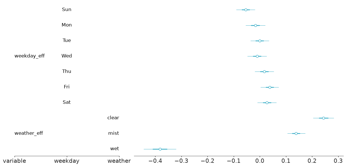
workingday- explain why you should not simply add it as well. - The effects in units the team can use: by what percentage does a wet day change demand relative to a clear one? How much did demand grow from 2011 to 2012? Which weekday is busiest? Do not forget the uncertainty.
- A PSIS-LOO comparison of all four models so far (
az.compare,az.plot_compare) and your reading of it: which steps mattered, judged byelpd_diffagainstdse? Read the warnings - you will come back to them in Task 5.
Solution
Coding. With dummy variables one weekday vanishes into the intercept and the prior
treats it differently from the other six (it has no coefficient, hence no prior
uncertainty of its own). pm.ZeroSumNormal gives every level an effect and constrains
them to sum to zero: effects are deviations from the average day, the intercept stays the
average day, and no level is special. We index the effect vector with the integer codes:
weekday_eff[weekday_idx].
Why not workingday as well? It is an exact function of the others:
workingday = not weekend and not holiday. Adding it gives the model two ways to say the
same thing; only the priors would hold the posterior together. Weekday effects plus a
holiday effect carry strictly more information.
Growth. The file offers yr, so the obvious first choice is a step: every 2012 day is
some percentage above the comparable 2011 day. We centre it (-0.5 / +0.5). Prior scales:
weekday effects of a few tens of percent at most (sigma=0.3), weather situations
possibly a halving (sigma=0.5), growth Normal(0, 1) per year because a young system
can plausibly double.
step_model = demand_model(train, calendar=True, trend="step")
step_idata = fit(step_model)
az.summary(step_idata, var_names=["~alpha", "~w_temp"], round_to=3)
divergences: 0 max r_hat: 1.007 min ess_bulk: 739
| mean | sd | eti89_lb | eti89_ub | ess_bulk | ess_tail | r_hat | mcse_mean | mcse_sd | |
|---|---|---|---|---|---|---|---|---|---|
| intercept | 8.142 | 0.021 | 8.109 | 8.175 | 1158.675 | 1558.045 | 1.002 | 0.001 | 0.000 |
| b_hum | -0.072 | 0.013 | -0.093 | -0.051 | 2301.483 | 2690.799 | 1.002 | 0.000 | 0.000 |
| b_wind | -0.088 | 0.010 | -0.104 | -0.073 | 5018.654 | 3197.073 | 1.001 | 0.000 | 0.000 |
| b_holiday | -0.098 | 0.060 | -0.195 | -0.004 | 5888.627 | 3118.086 | 1.000 | 0.001 | 0.001 |
| growth | 0.424 | 0.019 | 0.394 | 0.453 | 6312.089 | 3704.807 | 1.000 | 0.000 | 0.000 |
| weekday_eff[Sun] | -0.054 | 0.022 | -0.090 | -0.018 | 6116.909 | 3097.037 | 1.000 | 0.000 | 0.000 |
| weekday_eff[Mon] | -0.017 | 0.023 | -0.054 | 0.020 | 5676.370 | 3333.472 | 1.001 | 0.000 | 0.000 |
| weekday_eff[Tue] | -0.001 | 0.022 | -0.036 | 0.035 | 6841.480 | 3132.760 | 1.002 | 0.000 | 0.000 |
| weekday_eff[Wed] | -0.011 | 0.023 | -0.047 | 0.026 | 6812.623 | 2990.153 | 1.004 | 0.000 | 0.000 |
| weekday_eff[Thu] | 0.017 | 0.023 | -0.018 | 0.053 | 6863.603 | 3262.187 | 1.000 | 0.000 | 0.000 |
| weekday_eff[Fri] | 0.038 | 0.022 | 0.002 | 0.072 | 6247.629 | 3125.335 | 1.002 | 0.000 | 0.000 |
| weekday_eff[Sat] | 0.027 | 0.023 | -0.009 | 0.063 | 7362.155 | 2957.634 | 1.002 | 0.000 | 0.000 |
| weather_eff[clear] | 0.243 | 0.025 | 0.204 | 0.283 | 1177.713 | 1632.707 | 1.002 | 0.001 | 0.000 |
| weather_eff[mist] | 0.139 | 0.021 | 0.105 | 0.174 | 1766.479 | 2559.090 | 1.001 | 0.001 | 0.000 |
| weather_eff[wet] | -0.382 | 0.039 | -0.445 | -0.321 | 1104.572 | 1560.483 | 1.002 | 0.001 | 0.001 |
| cv | 0.236 | 0.007 | 0.226 | 0.247 | 6501.978 | 3153.149 | 1.001 | 0.000 | 0.000 |
def pct(x):
    return 100 * (np.exp(x) - 1)


def report(name, draws):
    lo, hi = np.quantile(draws, [0.03, 0.97])
    print(f"{name:<28} {draws.mean():+6.1f}%   94% interval [{lo:+.1f}, {hi:+.1f}]")


post = az.extract(step_idata)
wet_vs_clear = pct(post["weather_eff"].sel(weather="wet") - post["weather_eff"].sel(weather="clear")).values
mist_vs_clear = pct(post["weather_eff"].sel(weather="mist") - post["weather_eff"].sel(weather="clear")).values
growth_pct = pct(post["growth"]).values
report("wet day vs clear day", wet_vs_clear)
report("misty day vs clear day", mist_vs_clear)
report("public holiday", pct(post["b_holiday"]).values)
report("2012 vs 2011", growth_pct)
report("humidity +1 sd", pct(post["b_hum"]).values)
report("wind +1 sd", pct(post["b_wind"]).values)

az.plot_forest(step_idata, var_names=["weekday_eff", "weather_eff"], combined=True);
wet day vs clear day          -46.4%   94% interval [-52.5, -39.9]
misty day vs clear day         -9.9%   94% interval [-14.0, -5.5]
public holiday                 -9.2%   94% interval [-19.0, +1.7]
2012 vs 2011                  +52.8%   94% interval [+47.4, +58.2]
humidity +1 sd                 -6.9%   94% interval [-9.3, -4.6]
wind +1 sd                     -8.4%   94% interval [-10.1, -6.8]
train.groupby("weekday_name", observed=True)[["casual", "registered", "cnt"]].mean().round(0).T
| weekday_name | Sun | Mon | Tue | Wed | Thu | Fri | Sat |
|---|---|---|---|---|---|---|---|
| casual | 1385.0 | 693.0 | 570.0 | 571.0 | 607.0 | 765.0 | 1512.0 |
| registered | 2892.0 | 3627.0 | 3921.0 | 3964.0 | 4078.0 | 3914.0 | 3070.0 |
| cnt | 4277.0 | 4320.0 | 4490.0 | 4535.0 | 4685.0 | 4679.0 | 4582.0 |
assert h.check("task4", wet_vs_clear_pct=wet_vs_clear.mean(), growth_pct=growth_pct.mean())
- PASS
wet_vs_clear_pct= -46.41 is consistent with the reference solution. - PASS
growth_pct= 52.84 is consistent with the reference solution.
- A wet day costs 46% of demand relative to a clear day with the same temperature, humidity and wind (94% interval -52% to -40%); mist costs 10%.
- 2012 is 53% above 2011 (47% to 58%) at equal weather and calendar.
- Public holidays: about -9%, but the interval reaches zero - there are only 18 holidays in the training data.
- Once the weather situation is in the model the humidity coefficient shrinks from -0.18 to -0.07: the two carry much of the same information.
- Weekday effects are tiny: Sunday -5%, Friday +4%, everything else within a couple of percent of average. The table above shows why that is not the whole story: casual riders more than double at weekends while registered riders (commuters) drop by about a quarter, and in the total the two patterns almost cancel. A lead for "Going further".
cv is down to 0.24. Diagnostics are clean (no divergences, r_hat below 1.01). In the
table the smallest ESS (around 1,100) belongs to the intercept and the weather effects,
which trade off against each other because the levels are so unbalanced (64% of training
days are "clear", only 20 are "wet"); the slowest parameters overall are still the spline
weights, at about 740.
ladder = {
    "1 Poisson, linear weather": poisson_idata,
    "2 NegBin, linear weather": negbin_idata,
    "3 NegBin, temperature spline": spline_idata,
    "4 + calendar, weather, growth": step_idata,
}
loos = {name: az.loo(idata, pointwise=True) for name, idata in ladder.items()}  # compute once, reuse
az.compare(loos, round_to=1)
| rank | elpd_diff | dse | p_worse | diag_diff | diag_elpd | p | elpd | se | weight | |
|---|---|---|---|---|---|---|---|---|---|---|
| 4 + calendar, weather, growth | 0 | 0.0 | 0.0 | NaN | 1 k̂ > 0.70 | 30.4 | -5603.8 | 63.7 | 1.0 | |
| 3 NegBin, temperature spline | 1 | -204.6 | 34.1 | 1.0 | 12.6 | -5808.4 | 36.8 | 0.0 | ||
| 2 NegBin, linear weather | 2 | -305.3 | 43.4 | 1.0 | 6.7 | -5909.1 | 27.7 | 0.0 | ||
| 1 Poisson, linear weather | 3 | -169988.9 | 8724.7 | 1.0 | 133 k̂ > 0.70 | 1938.9 | -175592.7 | 8755.8 | 0.0 |
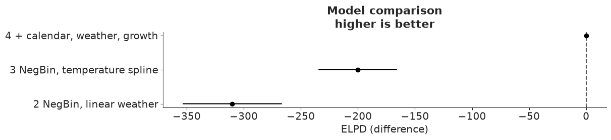
az.plot_compare(az.compare({k: v for k, v in loos.items() if "Poisson" not in k}));
# dse is always relative to the top row; for the spline-versus-line question compare just those two
az.compare({k: loos[k] for k in ["2 NegBin, linear weather", "3 NegBin, temperature spline"]}, round_to=1)[["elpd_diff", "dse", "p"]]
| elpd_diff | dse | p | |
|---|---|---|---|
| 3 NegBin, temperature spline | 0.0 | 0.0 | 12.6 |
| 2 NegBin, linear weather | -100.7 | 16.1 | 6.7 |
How to read the scoreboard:
- Poisson: 170,000 elpd behind. Not a typo. The log score punishes confident wrong
predictions without mercy, and a model that calls most days a one-in-a-billion event is
as confidently wrong as it gets. Its
p_looof about 1,900 for a model with 4 parameters and 133 bad Pareto-$k$ values say the same: the number itself is unreliable, the verdict is not. - Spline vs straight line: about 100 elpd, six times the
dseof that pair (16, second table). Remember thatdsein the big table is always relative to the top row. - Calendar, weather situation and growth: another 205 elpd, six times its
dseof 34. No surprise after Task 0, where the gap between the years was visible from across the room. - The best model has
p_looof 30 although it has only about 20 free parameters, and the table flags one observation with $\hat k > 0.7$. Something in the data has more influence than any single day should. That is Task 5.
Task 5 · The days the model cannot believe
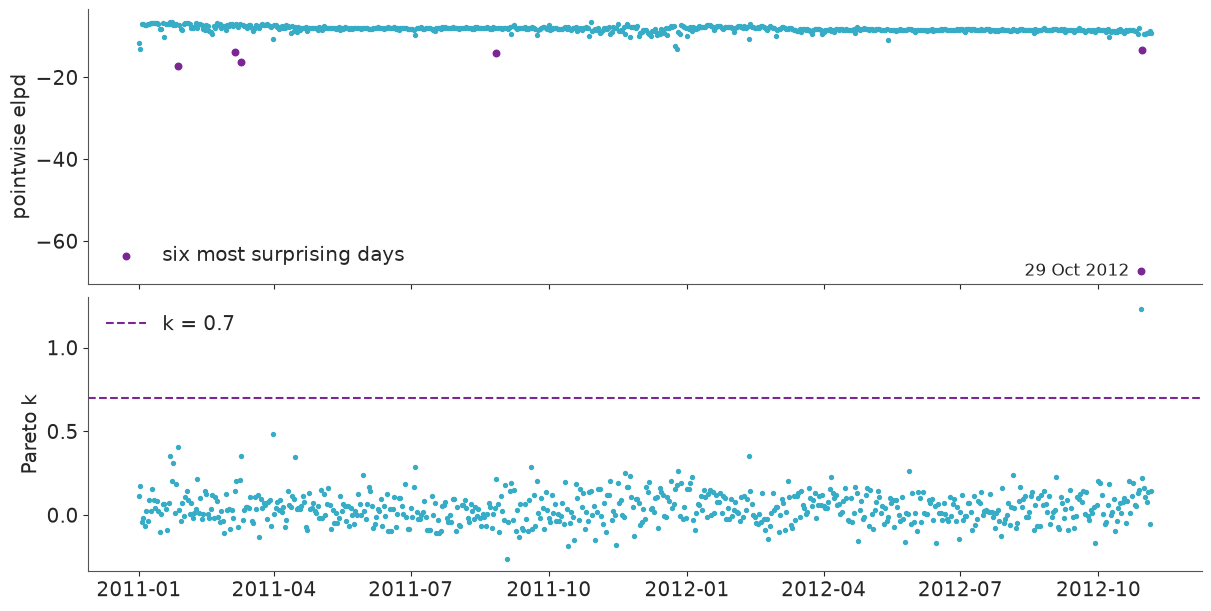
LOO is not only a scoreboard. It computes, for every single day, how well the model predicts that day when it has not seen it - and how much the posterior leans on it.
Deliver
- For your best model so far: the pointwise elpd and the Pareto-$k$ value of every training day, plotted against the date, and a table of the six most surprising days.
- For the worst of them: what happened? (You have the date and the internet.) Is it the kind of day the brief asks you to forecast? Look at the other five as well - is any of them a data problem rather than a demand problem?
- A decision on how to handle what you found, with a justification an auditor would accept, and a refit. What changed in the dispersion and in the width of the predictive intervals - and why does one day out of 675 have that much leverage?
loo4 = loos["4 + calendar, weather, growth"]
pointwise = train[["dteday", "cnt", "weather", "temp_c", "hum_pct", "wind_kmh"]].assign(
    predicted=step_idata.posterior_predictive["cnt"].mean(("chain", "draw")).values.round(),
    elpd=loo4.elpd_i.values,
    pareto_k=loo4.pareto_k.values,
)
surprising = pointwise.nsmallest(6, "elpd").set_index("dteday")

fig, axes = plt.subplots(2, 1, figsize=(12, 6), sharex=True)
axes[0].scatter(pointwise.dteday, pointwise.elpd, s=8)
axes[0].set(ylabel="pointwise elpd")
axes[1].scatter(pointwise.dteday, pointwise.pareto_k, s=8)
axes[1].axhline(0.7, color="C3", ls="--", label="k = 0.7")
axes[1].set(ylabel="Pareto k")
axes[1].legend()
axes[0].scatter(surprising.index, surprising.elpd, s=22, color="C3", label="six most surprising days")
axes[0].annotate(f"{surprising.index[0]:%d %b %Y}", (surprising.index[0], surprising.elpd.iloc[0]),
                 xytext=(-8, 0), textcoords="offset points", ha="right", va="center")
axes[0].legend(loc="lower left")

surprising.round(2)
| cnt | weather | temp_c | hum_pct | wind_kmh | predicted | elpd | pareto_k | |
|---|---|---|---|---|---|---|---|---|
| dteday | ||||||||
| 2012-10-29 | 22 | wet | 18.04 | 88.00 | 24.00 | 2176.0 | -67.36 | 1.23 |
| 2011-01-27 | 431 | clear | 8.00 | 68.75 | 7.63 | 1731.0 | -17.17 | 0.41 |
| 2011-03-10 | 623 | wet | 15.95 | 0.00 | 17.55 | 2157.0 | -16.27 | 0.36 |
| 2011-08-27 | 1115 | mist | 27.88 | 85.00 | 25.17 | 3215.0 | -13.99 | 0.21 |
| 2011-03-06 | 605 | mist | 15.44 | 94.83 | 23.00 | 1821.0 | -13.86 | 0.15 |
| 2012-10-30 | 1096 | mist | 13.05 | 82.55 | 14.27 | 3028.0 | -13.42 | 0.22 |
worst = pointwise.loc[pointwise.elpd.idxmin()]
assert h.check("task5", cnt_worst_day=worst.cnt, k_worst_day=worst.pareto_k)
- PASS
cnt_worst_day= 22 is consistent with the reference solution. - PASS
k_worst_day= 1.228 is consistent with the reference solution.
A typical day has a pointwise elpd of about -8 or -9. Then there is 29 October 2012: 22 rentals, elpd -67, Pareto-$k$ 1.2 - the only day beyond the 0.7 threshold. That is the day Hurricane Sandy reached Washington: the federal government and public transport shut down, and with 22 rentals in 24 hours the bike-share system was evidently closed too. The model sees "18 °C, wet, windy" and expects about 2,200 rentals. The next day (1,096 rentals where 3,000 were expected) is in the list as well.
The others are instructive in different ways:
- 27 January 2011 (431 rentals, "clear", 8 °C): the day after a heavy snowstorm. The sky was clear; the snow on the ground is not in the data.
- 27 August 2011: Hurricane Irene. 6 March 2011: 95% humidity and strong wind, but coded as "mist". For both, the three-level weather code understates how bad the day was.
- 10 March 2011: humidity of 0.00% on a wet day. That is not weather, that is a failed sensor - a data anomaly, which the model turned into a wrong prediction because it believed the number.
What to do. These are three different kinds of problem and deserve different answers:
- Sandy (29-30 October 2012): remove. On those days we did not observe demand, we observed a closed system. The brief is about staffing a system that operates; nobody needs a rebalancing plan for a hurricane shutdown. We state the condition - "forecasts assume normal operation" - rather than hide the deletion.
- The humidity reading: repair (interpolate between the neighbouring days). The day itself is fine.
- Snow, Irene, the wet "misty" day: keep. Bad days that the weather code describes poorly will happen again, and the predictive distribution should be wide enough to admit it. Deleting every day the model dislikes is how one ends up with beautifully narrow, wrong intervals.
SANDY = pd.to_datetime(["2012-10-29", "2012-10-30"])

train_clean = train[~train.dteday.isin(SANDY)].copy()
train_clean["hum_pct"] = train_clean.hum_pct.where(train_clean.hum_pct > 0).interpolate()  # sensor failure
print(f"humidity on 10 March 2011 after the repair: {train_clean.loc[train_clean.dteday == '2011-03-10', 'hum_pct'].item():.1f}%")

step_clean_model = demand_model(train_clean, calendar=True, trend="step")
step_clean_idata = fit(step_clean_model)
loo_step_clean = az.loo(step_clean_idata, pointwise=True)


def mean_width(idata, prob=0.9):
    lo, hi = interval(idata.posterior_predictive["cnt"], prob)
    return (hi - lo).mean()


for name, idata, loo in [("with Sandy", step_idata, loo4), ("without", step_clean_idata, loo_step_clean)]:
    print(
        f"{name:<11} cv = {float(idata.posterior['cv'].mean()):.3f}   alpha = {float(idata.posterior['alpha'].mean()):.1f}   "
        f"mean width of 90% interval = {mean_width(idata):.0f}   days with k > 0.7: {int((loo.pareto_k > 0.7).sum())}"
    )
humidity on 10 March 2011 after the repair: 71.2%
divergences: 0 max r_hat: 1.006 min ess_bulk: 783
with Sandy  cv = 0.236   alpha = 18.0   mean width of 90% interval = 3543   days with k > 0.7: 1
without     cv = 0.211   alpha = 22.4   mean width of 90% interval = 3185   days with k > 0.7: 0
Two days out of 675, and cv drops from 0.236 to 0.211 ($\alpha$ from 18 to 22); the average
90% interval narrows by 10% (3,543 to 3,185 rentals); no Pareto-$k$ above 0.7 remains.
Why so much leverage? The model has one dispersion parameter for all days. Under a negative binomial expecting a couple of thousand rentals, a count of 22 is astronomically unlikely unless $\alpha$ is small - so the likelihood buys a little plausibility for that one day by making every day noisier. That is exactly what a large Pareto-$k$ means: the posterior with and without this observation are different posteriors.
One caution: do not compare the elpd of this fit with the scoreboard of Task 4. The data are different (a day worth -67 is gone), so the totals are not comparable.
Task 6 · Open the hold-out
Time to find out whether "90%" means 90%. Forecast the 56 hold-out days with the model from Task 5, using the weather that actually occurred (a perfect weather forecast - the best case).
Deliver
- Forecasts produced without refitting: swap the inputs of the fitted model and sample the posterior predictive.
- A plot of the 50% and 90% predictive intervals against the actual counts, plus the empirical coverage of both intervals and the mean error (forecast median minus actual).
- If the forecasts are biased: find out why - not by tuning against the hold-out, but by asking what your growth term assumes about November 2012, and checking that assumption on the training data. Fix the model, compare old and new with LOO, and forecast again.
- A list of the hold-out days that still fall outside the 90% interval. What do they have in common? Could the training data have warned you? (Task 5 again.) Which direction is the error, and how much does that direction hurt the operations team?
def forecast(model, idata, new):
    """Posterior predictive draws of cnt for the rows of `new`, without refitting."""
    with model:
        pm.set_data(features(new), coords={"day": new.dteday.values})
        pred = pm.sample_posterior_predictive(idata, predictions=True, random_seed=RANDOM_SEED)
    return pred.predictions["cnt"]


def score(pp, y):
    median = pp.median(("chain", "draw")).values
    return {
        "coverage50": coverage(pp, y, 0.5),
        "coverage90": coverage(pp, y, 0.9),
        "mean error": float(np.mean(median - y)),
        "mean abs error": float(np.mean(np.abs(median - y))),
    }


def plot_forecast(pp, df, ax, title):
    y, dates = df.cnt.values, df.dteday.values
    lo90, hi90 = interval(pp, 0.9)
    lo50, hi50 = interval(pp, 0.5)
    outside = (y < lo90) | (y > hi90)
    ax.fill_between(dates, lo90, hi90, color="C0", alpha=0.25, lw=0, label="90%")
    ax.fill_between(dates, lo50, hi50, color="C0", alpha=0.5, lw=0, label="50%")
    ax.scatter(dates[~outside], y[~outside], s=14, color="k", zorder=3)
    ax.scatter(dates[outside], y[outside], s=14, color="C3", zorder=3, label="outside 90%")
    ax.set(ylabel="rentals per day", title=title, ylim=(0, 10500))
    ax.legend(ncols=3, loc="upper right")


pp_step = forecast(step_clean_model, step_clean_idata, test)
scores = {"step growth": score(pp_step, test.cnt.values)}
pd.DataFrame(scores).T.round(2)
| coverage50 | coverage90 | mean error | mean abs error | |
|---|---|---|---|---|
| step growth | 0.25 | 0.66 | -650.96 | 1151.63 |
fig, ax = plt.subplots(figsize=(12, 3.8))
plot_forecast(pp_step, test, ax, "Hold-out forecasts, step growth between years")
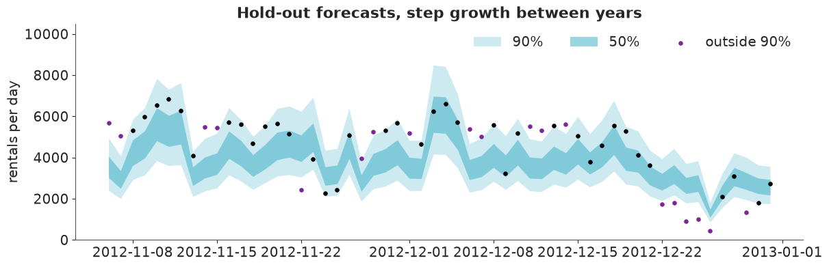
Not good. Only 66% of the hold-out days are inside the 90% interval and 25% inside the 50% interval. Worse, the errors are one-sided: the median forecast is on average 650 rentals too low, and before Christmas every miss but one is above the band. Under-forecasting is the expensive direction for the operations team.
The training coverage gave no hint of this. Nor would LOO: leaving out one day at a time tests interpolation - the neighbours of the missing day are still there. Forecasting is extrapolation in time, and only a hold-out at the end of the series tests that.
Why is the model biased? The growth term says "2012 is 53% above 2011" - one level per year. If the system actually grew steadily, that is too high for the start of each year and too low for the end. We can check that on the training data alone:
monthly = pd.DataFrame({"month": train_clean.dteday.dt.to_period("M").dt.to_timestamp(),
                        "res": log_residual(step_clean_idata, train_clean.cnt.values)}).groupby("month").res.mean()

fig, ax = plt.subplots(figsize=(11, 3.5))
ax.bar(monthly.index, monthly.values, width=20, color=np.where(monthly.values > 0, "C0", "C3"))
ax.axhline(0, color="k", lw=0.8)
ax.axvline(pd.Timestamp("2011-12-31"), color="k", ls=":", lw=1)
ax.set(ylabel="mean log(observed / predicted)", title="Monthly residuals of the step-growth model (training data)");
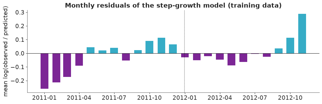
A saw-tooth. Within each year the residuals climb from negative to positive: -0.26 in January 2011, +0.11 by November 2011, back below zero in January 2012, and up to +0.11 in October 2012 (the last bar, +0.29, is only the first five days of November). The step model describes the average of 2012; the hold-out is the end of 2012.
The fix is a trend in continuous time: growth * t with t in years. It costs no extra
parameter.
final_model = demand_model(train_clean, calendar=True, trend="linear")
final_idata = fit(final_model)
az.summary(final_idata, var_names=["intercept", "growth", "b_holiday", "b_hum", "b_wind", "cv"], round_to=3)
divergences: 0 max r_hat: 1.005 min ess_bulk: 875
| mean | sd | eti89_lb | eti89_ub | ess_bulk | ess_tail | r_hat | mcse_mean | mcse_sd | |
|---|---|---|---|---|---|---|---|---|---|
| intercept | 8.170 | 0.017 | 8.143 | 8.198 | 882.212 | 1386.668 | 1.005 | 0.001 | 0.000 |
| growth | 0.463 | 0.015 | 0.438 | 0.487 | 4903.188 | 3110.141 | 1.000 | 0.000 | 0.000 |
| b_holiday | -0.117 | 0.048 | -0.193 | -0.038 | 5560.712 | 3092.677 | 1.001 | 0.001 | 0.001 |
| b_hum | -0.093 | 0.011 | -0.111 | -0.076 | 2032.121 | 2841.664 | 1.000 | 0.000 | 0.000 |
| b_wind | -0.064 | 0.008 | -0.077 | -0.051 | 3803.992 | 2777.460 | 1.001 | 0.000 | 0.000 |
| cv | 0.192 | 0.005 | 0.184 | 0.201 | 5775.052 | 3223.565 | 1.001 | 0.000 | 0.000 |
loo_final = az.loo(final_idata, pointwise=True)
az.compare({"step growth": loo_step_clean, "linear growth": loo_final}, round_to=1)
| rank | elpd_diff | dse | p_worse | diag_diff | diag_elpd | p | elpd | se | weight | |
|---|---|---|---|---|---|---|---|---|---|---|
| linear growth | 0 | 0.0 | 0.0 | NaN | 24.4 | -5447.8 | 33.5 | 0.8 | ||
| step growth | 1 | -62.3 | 17.9 | 1.0 | 23.1 | -5510.1 | 26.9 | 0.2 |
pp_final = forecast(final_model, final_idata, test)
scores["linear growth"] = score(pp_final, test.cnt.values)

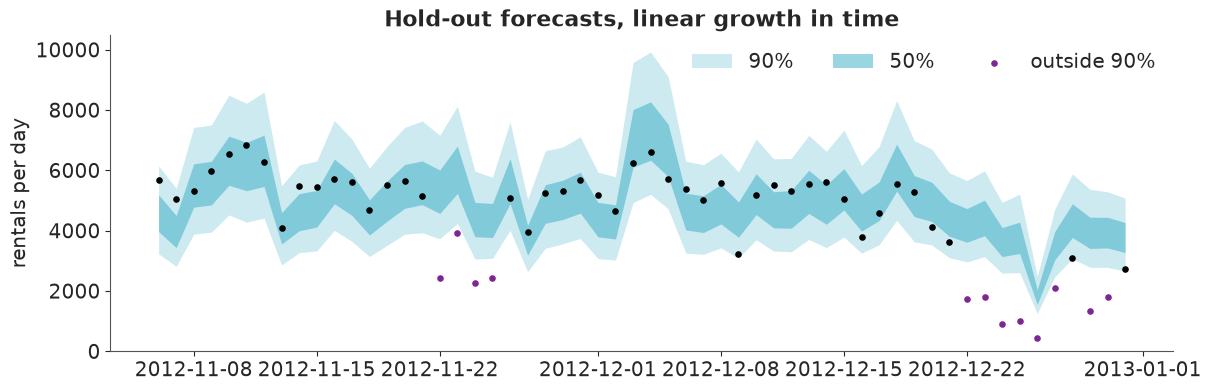
fig, ax = plt.subplots(figsize=(12, 3.8))
plot_forecast(pp_final, test, ax, "Hold-out forecasts, linear growth in time")
pd.DataFrame(scores).T.round(2)
| coverage50 | coverage90 | mean error | mean abs error | |
|---|---|---|---|---|
| step growth | 0.25 | 0.66 | -650.96 | 1151.63 |
| linear growth | 0.50 | 0.79 | 402.76 | 914.81 |
lo90, hi90 = interval(pp_final, 0.9)
missed = test.assign(lo90=lo90, hi90=hi90)[(test.cnt.values < lo90) | (test.cnt.values > hi90)]
missed.set_index("dteday")[["weekday_name", "holiday", "weather", "cnt", "lo90", "hi90"]].round(0)
| weekday_name | holiday | weather | cnt | lo90 | hi90 | |
|---|---|---|---|---|---|---|
| dteday | ||||||
| 2012-11-22 | Thu | 1 | clear | 2425 | 3732.0 | 7163.0 |
| 2012-11-23 | Fri | 0 | clear | 3910 | 4241.0 | 8128.0 |
| 2012-11-24 | Sat | 0 | clear | 2277 | 3060.0 | 5973.0 |
| 2012-11-25 | Sun | 0 | clear | 2424 | 3083.0 | 5769.0 |
| 2012-12-22 | Sat | 0 | clear | 1749 | 2964.0 | 5664.0 |
| 2012-12-23 | Sun | 0 | clear | 1787 | 3139.0 | 5984.0 |
| 2012-12-24 | Mon | 0 | mist | 920 | 2593.0 | 4937.0 |
| 2012-12-25 | Tue | 1 | mist | 1013 | 2608.0 | 5211.0 |
| 2012-12-26 | Wed | 0 | wet | 441 | 1251.0 | 2486.0 |
| 2012-12-27 | Thu | 0 | mist | 2114 | 2471.0 | 4713.0 |
| 2012-12-29 | Sat | 0 | mist | 1341 | 2786.0 | 5371.0 |
| 2012-12-30 | Sun | 0 | clear | 1796 | 2781.0 | 5289.0 |
print("most surprising TRAINING days under the final model:")
train_clean.assign(elpd=loo_final.elpd_i.values).nsmallest(6, "elpd").set_index("dteday")[["weekday_name", "weather", "cnt", "elpd"]].round(1)
most surprising TRAINING days under the final model:
| weekday_name | weather | cnt | elpd | |
|---|---|---|---|---|
| dteday | ||||
| 2011-12-25 | Sun | clear | 754 | -21.1 |
| 2011-01-27 | Thu | clear | 431 | -20.4 |
| 2011-12-24 | Sat | clear | 1011 | -19.5 |
| 2011-08-27 | Sat | mist | 1115 | -19.1 |
| 2011-03-06 | Sun | mist | 605 | -15.2 |
| 2011-12-27 | Tue | mist | 1162 | -14.4 |
holiday_season = (test.dteday.between("2012-11-22", "2012-11-25") | (test.dteday >= "2012-12-22")).values
ordinary = score(pp_final.isel(day=~holiday_season), test.cnt.values[~holiday_season])
print(f"{(~holiday_season).sum()} hold-out days outside Thanksgiving weekend and the Christmas period:")
print({k: round(v, 2) for k, v in ordinary.items()})

growth_per_year = pct(final_idata.posterior["growth"]).values.ravel()
print(f"growth: {growth_per_year.mean():.0f}% per year, 94% interval {np.quantile(growth_per_year, [0.03, 0.97]).round(0)}")
assert h.check(
    "task6",
    coverage90_first=scores["step growth"]["coverage90"],
    coverage90_final=scores["linear growth"]["coverage90"],
    growth_pct_per_year=growth_per_year.mean(),
)
42 hold-out days outside Thanksgiving weekend and the Christmas period:
{'coverage50': 0.67, 'coverage90': 1.0, 'mean error': -150.29, 'mean abs error': 532.45}
growth: 59% per year, 94% interval [54. 64.]- PASS
coverage90_first= 0.6607 is consistent with the reference solution. - PASS
coverage90_final= 0.7857 is consistent with the reference solution. - PASS
growth_pct_per_year= 58.87 is consistent with the reference solution.
- LOO prefers the linear trend by 62 elpd (3.5 times its
dse), with the same number of parameters, andcvfalls again, to 0.19 - still more than ten times the 1.5% that a Poisson model allows at 4,500 rentals a day. Growth is 59% per year (54% to 64%). Here LOO and the hold-out agree - but LOO alone did not tell us that the step model would forecast badly. - Hold-out: the 50% interval now covers 50% of days. The 90% interval covers 79%, and the bias has changed sign (+400).
- The 12 misses are all below the band and they are not random: Thanksgiving Thursday
to Sunday (22-25 November) and the Christmas period from 22 December. On the other 42
days the 90% interval covers every single day, the 50% interval two thirds of them, and
the mean error is -150: on ordinary days the intervals are, if anything, somewhat too
wide. (One shared
cvalso has to stretch over the festive and storm days in the training data.) - Could we have known? Yes. Under the final model the most surprising training days are
24, 25 and 27 December 2011. The
holidayflag marks single official holidays (-11%); it knows nothing about a city that empties for a week. One Christmas in the training data is thin evidence, but it was there, and pointwise LOO showed it. (First item in "Going further".) - Does it hurt? These errors are over-forecasts: vans and staff planned for riders who stayed at home. By the costs in the next task that is the cheap direction - but a team that sees the model miss ten days in a row will stop trusting it, so tell them in advance: in holiday weeks, plan below the model.
Task 7 · How much capacity?
The team plans three days in the coming weeks and hands you the weather forecast for each. (None is a public holiday.)
scenarios = pd.DataFrame(
    {
        "date": pd.to_datetime(["2012-11-16", "2012-11-18", "2012-11-20"]),
        "temp_c": [14.0, 8.0, 11.0],
        "hum_pct": [50.0, 70.0, 90.0],
        "wind_kmh": [10.0, 20.0, 15.0],
        "weather": ["clear", "mist", "wet"],
    },
    index=["mild clear Friday", "cold misty Sunday", "wet Tuesday"],
)
COST_LOST_RENTAL = 4.0  # $ per rental the system could not serve (lost fare and goodwill)
COST_IDLE = 0.5  # $ per unit of capacity planned but not used (vans, staff, bikes standing by)
scenarios
| date | temp_c | hum_pct | wind_kmh | weather | |
|---|---|---|---|---|---|
| mild clear Friday | 2012-11-16 | 14.0 | 50.0 | 10.0 | clear |
| cold misty Sunday | 2012-11-18 | 8.0 | 70.0 | 20.0 | mist |
| wet Tuesday | 2012-11-20 | 11.0 | 90.0 | 15.0 | wet |
Deliver
- For each scenario the capacity (in rentals per day) that covers demand with probability 95%, from your final model - and, next to it, the number you would get if you (wrongly) used only the uncertainty about the expected demand. How big is the gap?
- Management's 95% is a rule of thumb. With the two costs above, find the capacity that minimises expected cost for each scenario, numerically from the predictive draws. Which quantile of the predictive distribution does it correspond to? What ratio of the two costs would make the 95% rule optimal?
- Three sentences for the operations team: what to plan, how far to trust it, and when not to.
new = scenarios.assign(
    dteday=scenarios.date,
    weekday=(scenarios.date.dt.dayofweek + 1) % 7,  # pandas: Monday = 0; the file: Sunday = 0
    weathersit=[WEATHER.index(w) + 1 for w in scenarios.weather],
    holiday=0,
    yr=1,
    t=(scenarios.date - pd.Timestamp("2011-01-01")).dt.days / 365.25,
)
pp_new = forecast(final_model, final_idata, new)
draws = pp_new.stack(sample=("chain", "draw")).transpose("sample", "day").values  # (draws, 3 days)
def expected_demand(idata, df):
    """Posterior draws of mu (expected rentals) for the rows of df under the final model: (draws, rows)."""
    p = az.extract(idata)
    f = features(df)
    eta = (
        p["intercept"].values[:, None]
        + p["w_temp"].transpose("sample", "knot").values @ f["B"].T
        + p["b_hum"].values[:, None] * f["hum"]
        + p["b_wind"].values[:, None] * f["wind"]
        + p["weekday_eff"].transpose("sample", "weekday").values[:, f["weekday_idx"]]
        + p["weather_eff"].transpose("sample", "weather").values[:, f["weather_idx"]]
        + p["b_holiday"].values[:, None] * f["holiday"]
        + p["growth"].values[:, None] * f["t"]
    )
    return np.exp(eta)


mu_draws = expected_demand(final_idata, new)
capacity = pd.DataFrame(
    {
        "median forecast": np.median(draws, axis=0),
        "95% of expected demand (wrong)": np.quantile(mu_draws, 0.95, axis=0),
        "capacity95 (predictive)": np.quantile(draws, 0.95, axis=0),
    },
    index=scenarios.index,
)
capacity["safety margin"] = capacity["capacity95 (predictive)"] / capacity["median forecast"] - 1
capacity["P(shortfall) with the wrong number"] = (draws > capacity["95% of expected demand (wrong)"].values).mean(axis=0)
capacity.round({"median forecast": 0, "95% of expected demand (wrong)": 0, "capacity95 (predictive)": 0,
                "safety margin": 2, "P(shortfall) with the wrong number": 2})
| median forecast | 95% of expected demand (wrong) | capacity95 (predictive) | safety margin | P(shortfall) with the wrong number | |
|---|---|---|---|---|---|
| mild clear Friday | 5800.0 | 6146.0 | 7862.0 | 0.36 | 0.39 |
| cold misty Sunday | 2594.0 | 2813.0 | 3542.0 | 0.37 | 0.35 |
| wet Tuesday | 1909.0 | 2118.0 | 2613.0 | 0.37 | 0.29 |
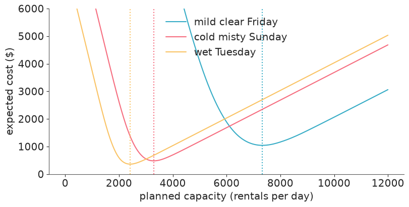
def expected_cost(capacity_grid, demand):
    """Expected cost of each capacity on the grid, averaging over predictive draws of demand."""
    short = np.clip(demand[None, :] - capacity_grid[:, None], 0, None)
    idle = np.clip(capacity_grid[:, None] - demand[None, :], 0, None)
    return (COST_LOST_RENTAL * short + COST_IDLE * idle).mean(axis=1)


grid = np.arange(0, 12001, 10)
fig, ax = plt.subplots(figsize=(8, 4))
for i, name in enumerate(scenarios.index):
    cost = expected_cost(grid, draws[:, i])
    best = grid[cost.argmin()]
    capacity.loc[name, "optimal capacity"] = best
    capacity.loc[name, "quantile of optimum"] = np.mean(draws[:, i] <= best)
    capacity.loc[name, "expected cost at optimum"] = cost.min()
    capacity.loc[name, "expected cost at capacity95"] = np.interp(capacity.loc[name, "capacity95 (predictive)"], grid, cost)
    ax.plot(grid, cost, color=f"C{i}", label=name)
    ax.axvline(best, color=f"C{i}", ls=":")
ax.set(xlabel="planned capacity (rentals per day)", ylabel="expected cost ($)", ylim=(0, 6000))
ax.legend()

critical_fractile = COST_LOST_RENTAL / (COST_LOST_RENTAL + COST_IDLE)
print(f"newsvendor critical fractile: {critical_fractile:.3f}")
capacity[["capacity95 (predictive)", "optimal capacity", "quantile of optimum",
          "expected cost at optimum", "expected cost at capacity95"]].round(2)
newsvendor critical fractile: 0.889
| capacity95 (predictive) | optimal capacity | quantile of optimum | expected cost at optimum | expected cost at capacity95 | |
|---|---|---|---|---|---|
| mild clear Friday | 7862.05 | 7330.0 | 0.89 | 1042.51 | 1122.75 |
| cold misty Sunday | 3542.05 | 3290.0 | 0.89 | 480.85 | 517.44 |
| wet Tuesday | 2613.05 | 2420.0 | 0.89 | 362.22 | 391.62 |
assert h.check(
    "task7",
    capacity95_friday=capacity.loc["mild clear Friday", "capacity95 (predictive)"],
    optimal_capacity_friday=capacity.loc["mild clear Friday", "optimal capacity"],
    optimal_quantile=capacity["quantile of optimum"].mean(),
)
- PASS
capacity95_friday= 7862 is consistent with the reference solution. - PASS
optimal_capacity_friday= 7330 is consistent with the reference solution. - PASS
optimal_quantile= 0.8896 is consistent with the reference solution.
Predictive, not posterior. For the mild Friday the median forecast is 5,800 rentals and the 95% capacity is about 7,900 - a safety margin of 36% (and the same 36-37% in the other scenarios, because negative-binomial scatter is proportional to the mean). The 95% quantile of the expected demand $\mu$ is only 6,150: it measures how well we know the average of many such Fridays, not how this Friday will turn out. Plan with it and you fall short on three to four such days in ten, not one in twenty (last column).
The 95% rule is a cost statement in disguise. Minimising expected cost over the predictive draws gives a capacity of about 7,330 for the Friday, which is the 0.89 quantile in every scenario - the newsvendor result $q^* = c_\text{short} / (c_\text{short} + c_\text{idle}) = 4 / 4.5$. The 95% rule costs about 8% more in expectation. It would be optimal if a lost rental cost 19 times as much as a unit of idle capacity ($0.95 = 19/20$). Maybe it does - empty docks make headlines - but that is for management to say, and now they can say it in dollars.
For the operations team:
- Plan for the model's 95% quantile - about a third above the central forecast - or for the 89% quantile if the two costs above are right; the forecast table gives both for any weather forecast you type in.
- On ordinary days the ranges have held up on eight weeks the model never saw. They assume the weather forecast is right, that the system operates normally, and that growth continues at the pace of 2011-2012 - the first assumption to re-check every few months, because nothing grows at 59% a year for long.
- Do not trust it around Thanksgiving and between Christmas and New Year, where it over-forecasts by a wide margin, and do not expect it to foresee a hurricane.
Going further
- Holiday seasons. The final model over-forecasts Thanksgiving weekend and the week after Christmas. Give it a way to learn that from 2011 (one Christmas is not much - what prior keeps the estimate honest?) and check whether hold-out coverage improves.
- Two populations.
casualandregisteredriders have opposite weekday patterns and different sensitivity to weather. Model them separately (or jointly, with shared growth) and add the predictive draws. Does the total forecast get sharper? - A Gaussian process instead of a spline. Replace the temperature spline with
pm.gp.HSGP, and the linear trend with a slowly-varying HSGP in time. Does the temperature curve change where data are sparse? What happens to forecasts when the trend is a GP that reverts to its mean? - The weather forecast is uncertain too. Tomorrow's temperature is known to within a couple of degrees and "wet" is a probability. Propagate that through the capacity decision by sampling scenarios. When does it matter?
h.progress()
C03: 0/23 hints used, 18/18 checks passed.