The brief
A survey-research team ran a moral-judgement study. Each participant read 30 short stories in which someone's action leads to a death, and rated how morally permissible the action was from 1 (absolutely not) to 7 (absolutely). The stories vary three features:
- action - the harm comes from doing something rather than from failing to act;
- intention - the death is a means to the agent's goal, not a side effect;
- contact - the agent physically touches the victim (in this coding contact stories are not also flagged as action).
The team analyses the ratings the way most survey teams do: ordinary linear regression on the numbers 1-7. A reviewer has told them that this is indefensible for Likert-type data. The team lead is unconvinced: "Everyone does it and the effects are huge. Show me one conclusion that would change."
Your job is to find out who is right - and to be honest about it in both directions.
How this notebook works
- Each task states what to deliver, not how. Write your code in the
YOUR CODE HEREcells. - Stuck?
h.hint("task2")reveals hints one level at a time: nudge → approach → code skeleton. Try to get by on nudges. h.check("task2", cut_first=...)compares your numbers with the reference solution.- A full worked solution lives in
notebooks/solutions/. Open it only when you are done (or truly stuck).
import arviz as az
import matplotlib.pyplot as plt
import numpy as np
import pandas as pd
import pymc as pm
from scipy import stats
from scipy.special import expit, logit

from pymc_challenges import Hints, data

RANDOM_SEED = 2006
rng = np.random.default_rng(RANDOM_SEED)
az.style.use("arviz-variat")

h = Hints("C05")
h.tasks()
C05 - Trolley problems: is a 1-7 rating a number?
task0- Look at the outcome (2 hints)task1- The team's linear model and a check that exposes it (3 hints, 2 check(s))task2- Ordered logistic, cutpoints only (3 hints, 2 check(s))task3- Ordinal regression with predictors (3 hints, 4 check(s))task4- Predictions on the response scale (3 hints, 3 check(s))task5- Participant and story effects (3 hints, 2 check(s))task6- Does the metric shortcut change a conclusion? (3 hints, 4 check(s))
The data
One row per rating. response is the 1-7 rating, id the participant, story one of 12
story settings (a boat, a burning building, a switch...), and action, intention,
contact the 0/1 features of the version of the story that was shown. age, male and
edu describe the participant.
data.describe("trolley")
trolley = data.load("trolley")
trolley.head()
trolley: 9930 ordinal (1-7) permissibility ratings from 331 participants.
  source: Cushman, Young & Hauser (2006) moral-judgement experiment, via `rethinking`.
  url:    https://raw.githubusercontent.com/rmcelreath/rethinking/master/data/Trolley.csv
| case | response | order | id | age | male | edu | action | intention | contact | story | action2 | |
|---|---|---|---|---|---|---|---|---|---|---|---|---|
| 0 | cfaqu | 4 | 2 | 96;434 | 14 | 0 | Middle School | 0 | 0 | 1 | aqu | 1 |
| 1 | cfbur | 3 | 31 | 96;434 | 14 | 0 | Middle School | 0 | 0 | 1 | bur | 1 |
| 2 | cfrub | 4 | 16 | 96;434 | 14 | 0 | Middle School | 0 | 0 | 1 | rub | 1 |
| 3 | cibox | 3 | 32 | 96;434 | 14 | 0 | Middle School | 0 | 1 | 1 | box | 1 |
| 4 | cibur | 3 | 4 | 96;434 | 14 | 0 | Middle School | 0 | 1 | 1 | bur | 1 |
Only six combinations of the three features occur in the experiment. We will call them scenarios and refer to them by these names throughout:
scenarios = pd.DataFrame(
    {"action": [0, 1, 0, 0, 1, 0], "intention": [0, 0, 0, 1, 1, 1], "contact": [0, 0, 1, 0, 0, 1]},
    index=pd.Index(
        ["none", "action", "contact", "intention", "action+intention", "contact+intention"],
        name="scenario",
    ),
)
key = ["action", "intention", "contact"]
trolley["scenario"] = pd.Categorical(
    trolley[key].merge(scenarios.reset_index(), on=key, how="left")["scenario"],
    categories=scenarios.index,
)
scenarios.assign(n=trolley.scenario.value_counts().reindex(scenarios.index))
| action | intention | contact | n | |
|---|---|---|---|---|
| scenario | ||||
| none | 0 | 0 | 0 | 1655 |
| action | 1 | 0 | 0 | 2648 |
| contact | 0 | 0 | 1 | 993 |
| intention | 0 | 1 | 0 | 1986 |
| action+intention | 1 | 1 | 0 | 1655 |
| contact+intention | 0 | 1 | 1 | 993 |
Task 0 · Look at the outcome
Deliver
- The distribution of
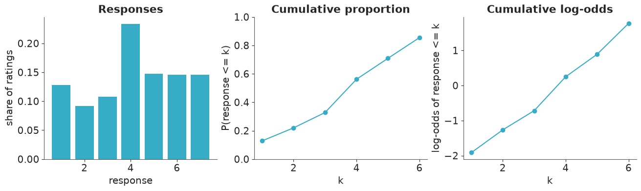
responseover its seven values, overall and for each scenario. - The cumulative proportions $P(\text{response} \le k)$ for $k = 1..6$ and the same numbers on the log-odds scale. Keep them - you will meet them again in Task 2.
- Two sentences: which features of this outcome will a Normal likelihood be unable to reproduce?
LEVELS = np.arange(1, 8)
obs_freq = trolley.response.value_counts(normalize=True).sort_index()
cum_prop = obs_freq.cumsum().iloc[:-1]
cum_logodds = logit(cum_prop)

fig, axes = plt.subplots(1, 3, figsize=(13, 3.8))
axes[0].bar(LEVELS, obs_freq, color="C0")
axes[0].set(xlabel="response", ylabel="share of ratings", title="Responses")
axes[1].plot(LEVELS[:-1], cum_prop, "o-")
axes[1].set(xlabel="k", ylabel="P(response <= k)", ylim=(0, 1), title="Cumulative proportion")
axes[2].plot(LEVELS[:-1], cum_logodds, "o-")
axes[2].set(xlabel="k", ylabel="log-odds of response <= k", title="Cumulative log-odds")

pd.DataFrame({"cum_prop": cum_prop, "cum_logodds": cum_logodds}).round(3).T
| response | 1 | 2 | 3 | 4 | 5 | 6 |
|---|---|---|---|---|---|---|
| cum_prop | 0.128 | 0.220 | 0.328 | 0.562 | 0.709 | 0.854 |
| cum_logodds | -1.916 | -1.267 | -0.719 | 0.248 | 0.890 | 1.769 |
scen_freq = pd.crosstab(trolley.scenario, trolley.response, normalize="index")
scen_mean = trolley.groupby("scenario", observed=True).response.mean()

fig, axes = plt.subplots(2, 3, figsize=(12, 5.5), sharex=True, sharey=True)
for ax, name in zip(axes.flat, scenarios.index):
    ax.bar(LEVELS, scen_freq.loc[name], color="C0")
    ax.axvline(scen_mean[name], color="k", ls="--", lw=1)
    ax.set_title(f"{name} (mean {scen_mean[name]:.2f})", fontsize=10)
fig.supxlabel("response")
fig.supylabel("share of ratings");
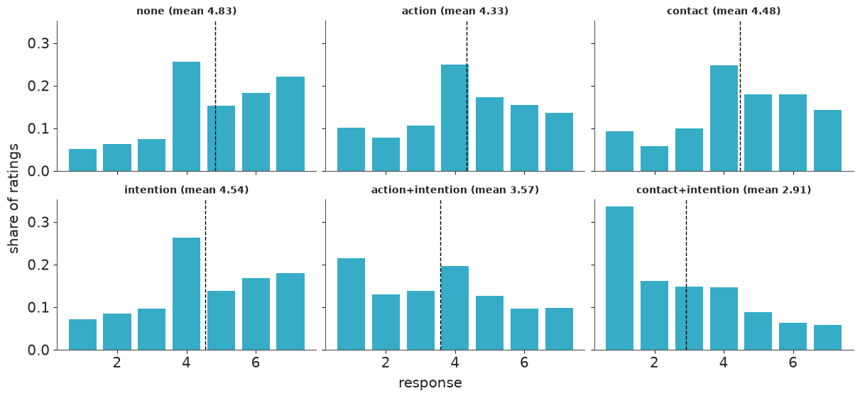
Nothing about this looks Normal. There is a spike at the midpoint 4 ("no opinion"), and the ends of the scale are piled up: 7 is as popular as 5 or 6 overall, and in contact+intention a third of all ratings sit on the floor at 1. A Normal has one hump, thin symmetric tails and no idea that 1 and 7 are walls. Notice also that the steps between consecutive cumulative log-odds are uneven - from 0.55 (between 2 and 3) to 0.97 (between 3 and 4). On the latent scale the categories are not equally wide, whereas treating 1-7 as a metric number assumes that every step is the same size.
Task 1 · The team's model
This is the model in the team's paper:
$$\text{response}_i \sim \text{Normal}(\mu_i, \sigma), \qquad \mu_i = a + b_A A_i + b_I I_i + b_C C_i + b_{AI} A_i I_i + b_{CI} C_i I_i$$
Deliver
- The fitted model with clean diagnostics.
- A posterior predictive check that you design to show the team what, if anything, is wrong with it. The responses are seven integers and the scenarios are very different from one another - a single smoothed density overlay will not do. Make the check reusable: you will want to run the same check on a better model later.
- One number for the abstract: what share of the model's predicted ratings are impossible (below 1 or above 7)?
Solution
The priors hardly matter with 9,930 rows; a is centred on the middle of the scale and the
slopes allow effects of a couple of rating points either way. One design matrix X is
shared by every model in this notebook.
COEFS = ["action", "intention", "contact", "action:intention", "contact:intention"]


def design(df):
    A, I, C = df.action.to_numpy(), df.intention.to_numpy(), df.contact.to_numpy()
    return np.column_stack([A, I, C, A * I, C * I]).astype(float)


X = design(trolley)
X_scen = design(scenarios)  # one row per scenario, for predictions
scen_idx = trolley.scenario.cat.codes.to_numpy()
scen_n = np.bincount(scen_idx)

with pm.Model(coords={"coef": COEFS}) as linear_model:
    a = pm.Normal("a", 4, 2)
    b = pm.Normal("b", 0, 1, dims="coef")
    sigma = pm.HalfNormal("sigma", 2)
    pm.Normal("response", a + pm.math.dot(X, b), sigma, observed=trolley.response.values)
    linear_idata = pm.sample(random_seed=RANDOM_SEED)

print("divergences:", int(linear_idata.sample_stats["diverging"].sum()))
az.summary(linear_idata, round_to=3)
divergences: 0
| mean | sd | eti89_lb | eti89_ub | ess_bulk | ess_tail | r_hat | mcse_mean | mcse_sd | |
|---|---|---|---|---|---|---|---|---|---|
| a | 4.831 | 0.044 | 4.760 | 4.900 | 1038.535 | 1505.796 | 1.003 | 0.001 | 0.001 |
| b[action] | -0.505 | 0.057 | -0.594 | -0.412 | 1136.954 | 1651.932 | 1.002 | 0.002 | 0.001 |
| b[intention] | -0.297 | 0.060 | -0.390 | -0.200 | 1034.789 | 1462.793 | 1.002 | 0.002 | 0.001 |
| b[contact] | -0.360 | 0.071 | -0.471 | -0.247 | 1603.831 | 1834.763 | 1.001 | 0.002 | 0.001 |
| b[action:intention] | -0.453 | 0.081 | -0.585 | -0.325 | 1254.365 | 1828.617 | 1.002 | 0.002 | 0.001 |
| b[contact:intention] | -1.264 | 0.099 | -1.425 | -1.107 | 1636.426 | 2433.184 | 1.003 | 0.002 | 0.001 |
| sigma | 1.816 | 0.013 | 1.796 | 1.837 | 4850.197 | 2646.732 | 1.001 | 0.000 | 0.000 |
The sampler is perfectly happy, the intervals are tight, every effect is "significant". None of that says anything about whether the model can produce data like ours.
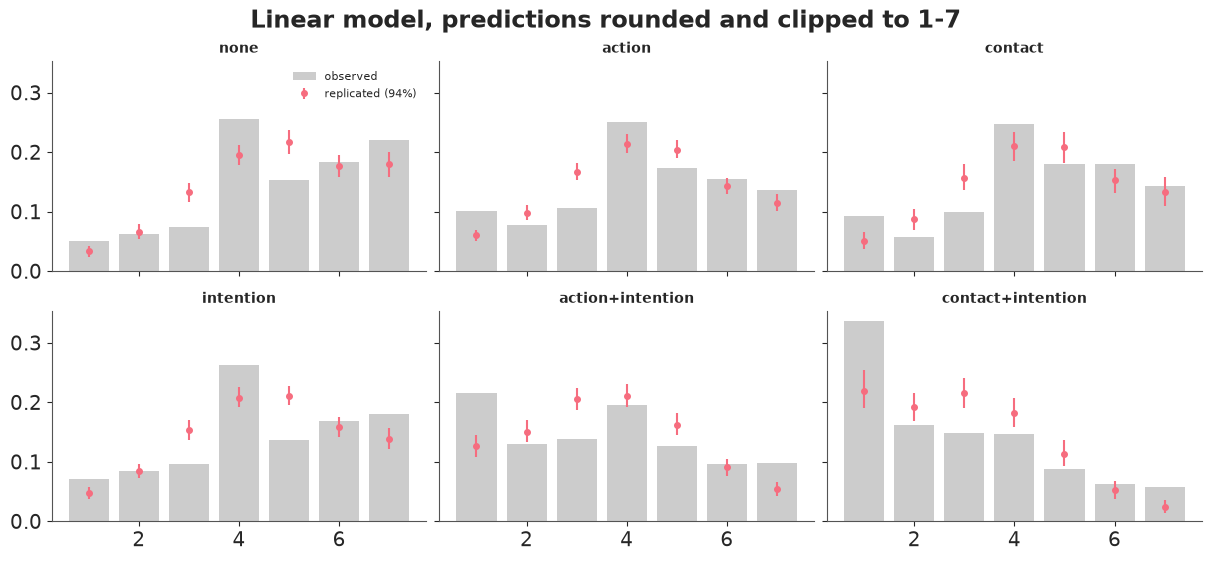
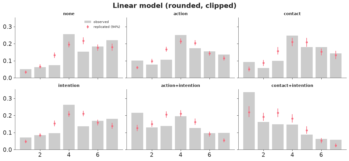
The check. Simulate replicated datasets and compare, scenario by scenario, the share of ratings in each of the seven categories. The linear model predicts real numbers, so to give it the best possible chance we round its predictions to the nearest integer and clip them to 1-7 - and separately count how often that clipping was needed.
Within a scenario every row has the same $\mu$, so we only need to simulate n ratings per
scenario and posterior draw, not push 9,930 x 4,000 numbers through
pm.sample_posterior_predictive.
N_REP = 400  # posterior draws used for replicated datasets


def category_freq(y_rep):
    """Share of ratings 1..7 in an array of integer ratings."""
    return np.bincount(y_rep.astype(int), minlength=8)[1:] / y_rep.size


def linear_replicates(idata, n_rep=N_REP):
    """Raw (continuous) replicated ratings per scenario: list of arrays (n_rep, n_scenario_rows)."""
    post = az.extract(idata, num_samples=n_rep, random_seed=RANDOM_SEED)
    mu = post["a"].values[:, None] + post["b"].values.T @ X_scen.T  # (n_rep, 6)
    return [rng.normal(mu[:, [s]], post["sigma"].values[:, None], size=(n_rep, scen_n[s])) for s in range(6)]


def plot_ppc_categories(freq_rep, title, color="C1", axes=None):
    """freq_rep: (n_rep, 6 scenarios, 7 categories) replicated category shares."""
    if axes is None:
        _, axes = plt.subplots(2, 3, figsize=(12, 5.5), sharex=True, sharey=True)
    lo, hi = np.quantile(freq_rep, [0.03, 0.97], axis=0)
    mid = freq_rep.mean(axis=0)
    for s, (ax, name) in enumerate(zip(axes.flat, scenarios.index)):
        ax.bar(LEVELS, scen_freq.loc[name], color="0.8", label="observed")
        ax.errorbar(LEVELS, mid[s], yerr=[mid[s] - lo[s], hi[s] - mid[s]], fmt="o", ms=4, color=color,
                    label="replicated (94%)")
        ax.set_title(name, fontsize=10)
    axes.flat[0].legend(fontsize=8)
    axes.flat[0].figure.suptitle(title)
    return axes


raw = linear_replicates(linear_idata)
linear_freq = np.stack(
    [[category_freq(np.clip(np.rint(r), 1, 7)) for r in raw_s] for raw_s in raw], axis=1
)  # (n_rep, 6, 7)
plot_ppc_categories(linear_freq, "Linear model, predictions rounded and clipped to 1-7");
all_raw = np.concatenate(raw, axis=1)
share_impossible = ((all_raw < 1) | (all_raw > 7)).mean()
by_scen = pd.Series([((r < 1) | (r > 7)).mean() for r in raw], index=scenarios.index)
print(f"share of predicted ratings below 1 or above 7: {share_impossible:.3f}")
print(by_scen.round(3).to_string())
share of predicted ratings below 1 or above 7: 0.118
scenario
none                 0.134
action               0.104
contact              0.111
intention            0.113
action+intention     0.107
contact+intention    0.159
assert h.check(
    "task1",
    sigma=linear_idata.posterior["sigma"].mean(),
    share_impossible=share_impossible,
)
- PASS
sigma= 1.816 is consistent with the reference solution. - PASS
share_impossible= 0.1175 is consistent with the reference solution.
Even with rounding and clipping in its favour, the linear model gets the shape wrong in every scenario, and always in the same way: too many 3s and 5s, too few 4s, and too little mass at the ends of the scale. It is worst where the mean is closest to a wall: in contact+intention it expects about 22% of ratings to be a 1 when 34% are, and it under-predicts 7s in none. And 12% of its raw predictions are ratings that cannot exist (16% in contact+intention).
Note what the check did not show: the means. Those are fine, as Task 6 will confirm. A posterior predictive check only exposes what you ask it about.
Task 2 · An ordinal likelihood
Leave the predictors aside for a moment. Model the seven categories as an ordered logistic outcome: a latent continuous "permissibility" with a logistic distribution, cut into seven bins by six cutpoints.
Deliver
- Before fitting: what does your prior on the cutpoints imply for the seven category probabilities? Show it.
- The fitted intercept-only model with clean diagnostics. If your first attempt dies before a single draw is taken, do not reach for a different sampler - find out which term of the log-probability is to blame at the starting point, and fix the model.
- Compare the posterior cutpoints with a number you already have from Task 0. What are the cutpoints, in words?
Solution
pm.OrderedLogistic wants categories coded 0..6 and defines
$P(y \le k) = \text{logistic}(c_k - \eta)$. The category probabilities are differences of
consecutive cumulative probabilities, so they are only non-negative if
$c_1 < c_2 < \dots < c_6$. Here is what happens when nobody tells the sampler that:
y = trolley.response.values - 1  # 0..6
CUTS = [f"{k}|{k + 1}" for k in range(1, 7)]

with pm.Model(coords={"cutpoint": CUTS}) as unordered_model:
    cut = pm.Normal("cut", 0, 1.5, dims="cutpoint")
    pm.OrderedLogistic("response", eta=0.0, cutpoints=cut, observed=y)

print("log-probability at the starting point:", unordered_model.point_logps())
try:
    with unordered_model:
        pm.sample(random_seed=RANDOM_SEED)
except Exception as err:  # noqa: BLE001
    print(f"\n{type(err).__name__}: {str(err)[:300]}")
log-probability at the starting point: {'cut': np.float64(-7.95), 'response': np.float64(-inf)}RuntimeError: All initialization points failed
Caused by:
Logp function returned error: ErrorCode(4)The default starting point puts all six cutpoints at 0. Every interior category then has
probability logistic(0) - logistic(0) = 0, the data contain thousands of them, and the
log-likelihood is -inf. Jittering the start does not help: almost every random
permutation of six numbers is out of order, which gives negative probabilities.
The cure has two parts, and you need both:
transform=pm.distributions.transforms.orderedmakes the sampler work with $(c_1, \log(c_2 - c_1), \dots)$, so every point it visits is ordered;- an ordered starting value. The transform takes the log of the gaps, and the default
start (all zeros) has gaps of zero - so with the transform alone the model still fails,
now with
-infin the prior term as well.
ordered = pm.distributions.transforms.ordered
CUT_INIT = np.linspace(-2, 2, 6)

with pm.Model(coords={"cutpoint": CUTS}) as transform_only:
    cut = pm.Normal("cut", 0, 1.5, dims="cutpoint", transform=ordered)
    pm.OrderedLogistic("response", eta=0.0, cutpoints=cut, observed=y)
print("ordered transform, default start:", transform_only.point_logps())
ordered transform, default start: {'cut': np.float64(-inf), 'response': np.float64(-inf)}Prior. On the log-odds scale ±4 already means 2% and 98%, so Normal(0, 1.5) for each
cutpoint is weakly informative. With the ordered transform the prior is that density
restricted to ordered vectors - which is the distribution of six sorted independent
draws. (pm.sample_prior_predictive ignores transforms and would hand you unsorted
cutpoints, so we do this one by hand.)
def ordinal_probs(eta, cut):
    """Category probabilities. eta: (...,), cut: (..., 6) -> (..., 7)."""
    cdf = expit(cut - np.asarray(eta)[..., None])
    cdf = np.concatenate([np.zeros_like(cdf[..., :1]), cdf, np.ones_like(cdf[..., :1])], axis=-1)
    return np.diff(cdf, axis=-1)


prior_cut = np.sort(rng.normal(0, 1.5, size=(500, 6)), axis=1)
prior_p = ordinal_probs(np.zeros(500), prior_cut)

fig, ax = plt.subplots(figsize=(6, 3.5))
ax.plot(LEVELS, prior_p[:80].T, color="C0", alpha=0.2)
ax.plot(LEVELS, prior_p.mean(axis=0), "k-o", label="prior mean")
ax.set(xlabel="response", ylabel="probability", title="Category probabilities implied by the prior")
ax.legend();
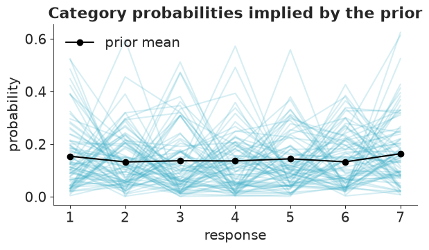
On average the prior spreads probability almost evenly over the seven categories (about 1/7 each), while single draws range from nearly empty categories to ones holding more than half of the mass. That is as vague as we want to be: nothing is ruled out, and no category is favoured.
with pm.Model(coords={"cutpoint": CUTS}) as cut_model:
    cut = pm.Normal("cut", 0, 1.5, dims="cutpoint", transform=ordered)
    pm.OrderedLogistic("response", eta=0.0, cutpoints=cut, observed=y)
    cut_idata = pm.sample(initvals={"cut": CUT_INIT}, random_seed=RANDOM_SEED)

print("divergences:", int(cut_idata.sample_stats["diverging"].sum()))
az.summary(cut_idata, var_names=["cut"], round_to=3)
divergences: 0
| mean | sd | eti89_lb | eti89_ub | ess_bulk | ess_tail | r_hat | mcse_mean | mcse_sd | |
|---|---|---|---|---|---|---|---|---|---|
| cut[1|2] | -1.917 | 0.031 | -1.966 | -1.867 | 2969.036 | 2609.905 | 1.001 | 0.001 | 0.0 |
| cut[2|3] | -1.267 | 0.024 | -1.305 | -1.229 | 4170.231 | 2927.030 | 1.000 | 0.000 | 0.0 |
| cut[3|4] | -0.718 | 0.021 | -0.752 | -0.686 | 4823.500 | 3728.625 | 1.000 | 0.000 | 0.0 |
| cut[4|5] | 0.248 | 0.020 | 0.214 | 0.281 | 5937.256 | 3977.919 | 1.001 | 0.000 | 0.0 |
| cut[5|6] | 0.890 | 0.022 | 0.855 | 0.924 | 5835.405 | 3543.553 | 1.001 | 0.000 | 0.0 |
| cut[6|7] | 1.770 | 0.028 | 1.726 | 1.813 | 6194.230 | 4059.326 | 1.002 | 0.000 | 0.0 |
cut_mean = cut_idata.posterior["cut"].mean(("chain", "draw")).values
print(pd.DataFrame({"posterior mean": cut_mean, "empirical log-odds": cum_logodds.values}, index=CUTS).round(3))
assert h.check("task2", cut_first=cut_mean[0], cut_last=cut_mean[-1])
     posterior mean  empirical log-odds
1|2          -1.917              -1.916
2|3          -1.267              -1.267
3|4          -0.718              -0.719
4|5           0.248               0.248
5|6           0.890               0.890
6|7           1.770               1.769
- PASS
cut_first= -1.917 is consistent with the reference solution. - PASS
cut_last= 1.77 is consistent with the reference solution.
The posterior means reproduce the empirical cumulative log-odds from Task 0 to within 0.001. With no predictors that is all the cutpoints are: the log-odds of responding at most k, six free numbers that can match any histogram over seven categories. The spike at 4 and the pile-ups at 1 and 7 cost this model nothing. Everything that follows keeps that flexibility and lets predictors shift the whole latent scale.
Task 3 · Ordinal regression
Add the team's predictors - action, intention, contact and the two interactions with intention - to the ordinal model, with the convention that a positive coefficient means "more permissible".
Deliver
- Priors for the coefficients that you can defend on the log-odds scale.
- The fitted model with clean diagnostics. (Memory warning: by default
pm.OrderedLogisticstores the seven category probabilities of every row for every draw. With 9,930 rows that is gigabytes. Find the switch.) - Your Task 1 check, run on this model and shown next to the linear one.
Solution
A coefficient of 1 on the log-odds scale is a large effect: it moves a 50% cumulative
probability to 27%. Normal(0, 0.5) says effects beyond ±1 are unlikely but possible.
There is no intercept: the six cutpoints already are six intercepts, and adding a
seventh would make the model non-identified.
with pm.Model(coords={"cutpoint": CUTS, "coef": COEFS}) as ordinal_model:
    cut = pm.Normal("cut", 0, 1.5, dims="cutpoint", transform=ordered)
    b = pm.Normal("b", 0, 0.5, dims="coef")
    pm.OrderedLogistic("response", eta=pm.math.dot(X, b), cutpoints=cut, observed=y, compute_p=False)
    ordinal_idata = pm.sample(initvals={"cut": CUT_INIT}, random_seed=RANDOM_SEED)

print("divergences:", int(ordinal_idata.sample_stats["diverging"].sum()))
az.summary(ordinal_idata, round_to=3)
divergences: 0
| mean | sd | eti89_lb | eti89_ub | ess_bulk | ess_tail | r_hat | mcse_mean | mcse_sd | |
|---|---|---|---|---|---|---|---|---|---|
| b[action] | -0.470 | 0.054 | -0.555 | -0.384 | 1538.959 | 1811.296 | 1.001 | 0.001 | 0.001 |
| b[intention] | -0.289 | 0.057 | -0.382 | -0.199 | 1459.904 | 1789.584 | 1.002 | 0.001 | 0.001 |
| b[contact] | -0.340 | 0.068 | -0.448 | -0.230 | 1715.576 | 2217.699 | 1.001 | 0.002 | 0.001 |
| b[action:intention] | -0.438 | 0.078 | -0.562 | -0.311 | 1759.739 | 2137.349 | 1.000 | 0.002 | 0.001 |
| b[contact:intention] | -1.240 | 0.098 | -1.396 | -1.087 | 1862.529 | 2345.156 | 1.001 | 0.002 | 0.001 |
| cut[1|2] | -2.630 | 0.052 | -2.715 | -2.549 | 1285.449 | 1530.077 | 1.001 | 0.001 | 0.001 |
| cut[2|3] | -1.935 | 0.048 | -2.012 | -1.860 | 1382.083 | 1651.057 | 1.002 | 0.001 | 0.001 |
| cut[3|4] | -1.341 | 0.046 | -1.414 | -1.269 | 1436.048 | 1635.069 | 1.002 | 0.001 | 0.001 |
| cut[4|5] | -0.307 | 0.044 | -0.377 | -0.237 | 1429.515 | 1717.955 | 1.003 | 0.001 | 0.001 |
| cut[5|6] | 0.364 | 0.043 | 0.294 | 0.433 | 1463.234 | 1981.270 | 1.002 | 0.001 | 0.001 |
| cut[6|7] | 1.270 | 0.046 | 1.194 | 1.341 | 1697.249 | 2145.609 | 1.004 | 0.001 | 0.001 |
def scenario_probs(idata, num_samples=None):
    """Posterior category probabilities per scenario: (draws, 6 scenarios, 7 categories)."""
    post = az.extract(idata, var_names=["b", "cut"], num_samples=num_samples, random_seed=RANDOM_SEED)
    eta = post["b"].values.T @ X_scen.T  # (draws, 6)
    return ordinal_probs(eta, post["cut"].values.T[:, None, :])


p_rep = scenario_probs(ordinal_idata, num_samples=N_REP)
ordinal_freq = np.stack(
    [[rng.multinomial(scen_n[s], p_draw[s]) / scen_n[s] for s in range(6)] for p_draw in p_rep]
)  # (n_rep, 6, 7)

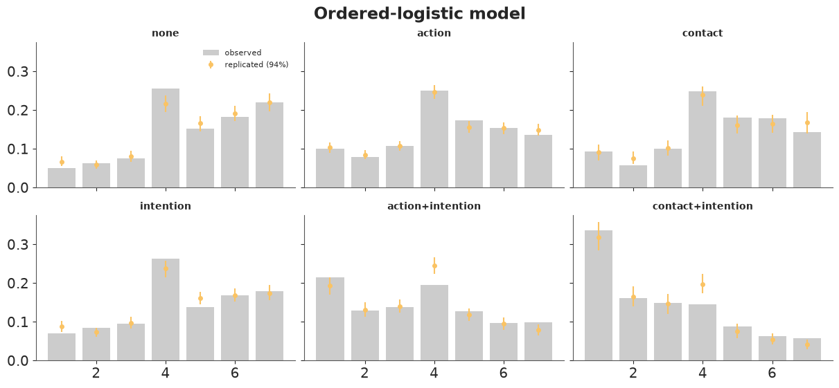
plot_ppc_categories(linear_freq, "Linear model (rounded, clipped)", color="C1")
plot_ppc_categories(ordinal_freq, "Ordered-logistic model", color="C2");
def ppc_error(freq_rep):
    """Mean absolute error of the replicated category shares, in percentage points, per scenario."""
    err = np.abs(freq_rep.mean(axis=0) - scen_freq.values).mean(axis=1) * 100
    return pd.Series(err, index=scenarios.index)


pd.DataFrame({"linear": ppc_error(linear_freq), "ordinal": ppc_error(ordinal_freq)}).round(2)
| linear | ordinal | |
|---|---|---|
| scenario | ||
| none | 3.57 | 1.23 |
| action | 3.15 | 0.62 |
| contact | 3.30 | 1.28 |
| intention | 3.72 | 1.23 |
| action+intention | 3.99 | 1.52 |
| contact+intention | 4.59 | 1.58 |
b_mean = ordinal_idata.posterior["b"].mean(("chain", "draw"))
assert h.check(
    "task3",
    b_action=b_mean.sel(coef="action"),
    b_intention=b_mean.sel(coef="intention"),
    b_contact=b_mean.sel(coef="contact"),
    b_contact_intention=b_mean.sel(coef="contact:intention"),
)
- PASS
b_action= -0.4702 is consistent with the reference solution. - PASS
b_intention= -0.2888 is consistent with the reference solution. - PASS
b_contact= -0.34 is consistent with the reference solution. - PASS
b_contact_intention= -1.24 is consistent with the reference solution.
All five coefficients are negative: every feature makes the act less permissible, and intention combined with contact (-1.24) far more than the sum of its parts.
On the same check the ordinal model cuts the average error in the category shares from 3-5 percentage points to 0.6-1.6, and it cannot produce an impossible rating. The floor in contact+intention and the ceiling in none are now reproduced.
It is not perfect, and the check shows where: in the two harshest scenarios it predicts too many 4s (about 24% against 20% observed in action+intention, 20% against 15% in contact+intention). The model assumes proportional odds - predictors slide the whole latent distribution past fixed cutpoints - but people who condemn these acts seem to abandon the neutral midpoint faster than that allows. That is a lead for "Going further", and a much smaller problem than the one we started with.
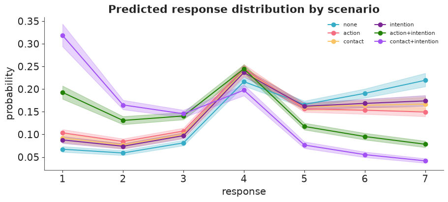
Task 4 · Back to the scale people answered on
"The contact:intention coefficient is -1.2 on the latent log-odds scale" is not a sentence you can put in front of the survey team.
Deliver, from the ordinal model, with 94% intervals:
- A figure of the predicted distribution over the seven categories for each scenario.
- A table with the expected rating and $P(\text{response} \le 3)$ ("leans impermissible") for each scenario.
- The headline contrast: going from none to contact+intention, how much does the expected rating fall, and by how many percentage points does $P(\text{response} \le 3)$ rise?
P_ord = scenario_probs(ordinal_idata)  # (draws, 6, 7)
mean_ord = (P_ord * LEVELS).sum(axis=-1)  # (draws, 6)
le3_ord = P_ord[..., :3].sum(axis=-1)


def summarise(draws, index, name):
    lo, hi = np.quantile(draws, [0.03, 0.97], axis=0)
    return pd.DataFrame({name: draws.mean(axis=0), "lo": lo, "hi": hi}, index=index)


fig, ax = plt.subplots(figsize=(9, 4))
lo, hi = np.quantile(P_ord, [0.03, 0.97], axis=0)
for s, name in enumerate(scenarios.index):
    ax.plot(LEVELS, P_ord[:, s].mean(axis=0), "o-", color=f"C{s}", label=name)
    ax.fill_between(LEVELS, lo[s], hi[s], color=f"C{s}", alpha=0.25)
ax.set(xlabel="response", ylabel="probability", title="Predicted response distribution by scenario")
ax.legend(fontsize=8, ncol=2);
pd.concat(
    {
        "expected rating": summarise(mean_ord, scenarios.index, "mean"),
        "P(response <= 3)": summarise(le3_ord, scenarios.index, "mean"),
    },
    axis=1,
).round(3)
| expected rating | P(response <= 3) | |||||
|---|---|---|---|---|---|---|
| mean | lo | hi | mean | lo | hi | |
| scenario | ||||||
| none | 4.804 | 4.727 | 4.884 | 0.207 | 0.194 | 0.222 |
| action | 4.325 | 4.258 | 4.392 | 0.295 | 0.281 | 0.310 |
| contact | 4.460 | 4.353 | 4.563 | 0.269 | 0.249 | 0.291 |
| intention | 4.512 | 4.438 | 4.587 | 0.259 | 0.244 | 0.274 |
| action+intention | 3.563 | 3.478 | 3.649 | 0.464 | 0.443 | 0.485 |
| contact+intention | 2.881 | 2.775 | 2.987 | 0.629 | 0.602 | 0.655 |
NONE, CI = 0, 5  # positions of "none" and "contact+intention" in `scenarios`
shift_mean = mean_ord[:, CI] - mean_ord[:, NONE]
shift_le3 = le3_ord[:, CI] - le3_ord[:, NONE]
for label, d, scale in [("expected rating", shift_mean, 1), ("P(response <= 3), pct points", shift_le3, 100)]:
    print(f"none -> contact+intention, {label}: {scale * d.mean():.2f} "
          f"[{scale * np.quantile(d, 0.03):.2f}, {scale * np.quantile(d, 0.97):.2f}]")

assert h.check(
    "task4",
    mean_none=mean_ord[:, NONE].mean(),
    p_le3_contact_intention=le3_ord[:, CI].mean(),
    shift_mean=shift_mean.mean(),
)
none -> contact+intention, expected rating: -1.92 [-2.06, -1.79]
none -> contact+intention, P(response <= 3), pct points: 42.14 [39.18, 45.07]
- PASS
mean_none= 4.804 is consistent with the reference solution. - PASS
p_le3_contact_intention= 0.6289 is consistent with the reference solution. - PASS
shift_mean= -1.923 is consistent with the reference solution.
In the team's language: with none of the three features present the expected rating is 4.8 and about one rating in five leans impermissible (3 or lower). When the death is intended and involves physical contact, the expected rating falls by 1.9 points to 2.9, and the share leaning impermissible triples to 63% - a rise of 42 percentage points (94% interval 39-45). Almost a third of respondents then choose the very lowest category.
Everything here was computed per posterior draw and summarised last, which is why each number comes with an interval. Coefficients on the latent scale have no such direct reading: the same shift in $\eta$ moves more or less probability depending on where the cutpoints are.
Task 5 · People differ
Every participant rated 30 stories, and so far the models have treated their 30 answers as independent. Some people are strict, some lenient; some stories are simply more upsetting than others whatever their features.
To stay inside a laptop runtime budget this task uses a random subsample of 150 participants (4,500 ratings), defined below. Use it for every model in this task so that they can be compared.
Deliver
- An ordinal model with a varying intercept per participant and an effect per story, with clean diagnostics. 150 correlated intercepts next to six cutpoints is a location-identification problem waiting to happen - deal with it in the model.
- How large is the between-participant standard deviation compared with the biggest treatment effect? Put it in words.
- A LOO comparison with the Task 3 model refitted to the same subsample. How much do the participant and story effects matter for prediction?
- Put the coefficients of the two models side by side. They all moved away from zero. Explain why that is expected and not a contradiction.
# a dedicated generator, so that everybody gets the same 150 people whatever was run before
sub_ids = np.sort(np.random.default_rng(RANDOM_SEED).choice(trolley.id.unique(), size=150, replace=False))
sub = trolley[trolley.id.isin(sub_ids)].reset_index(drop=True)
print(f"{sub.id.nunique()} participants, {len(sub)} ratings")
150 participants, 4500 ratings
Solution
The cutpoints fix the location of the latent scale, so the participant and story effects
must not be able to shift it as well. pm.ZeroSumNormal builds the sum-to-zero constraint
into the prior, which removes that ridge from the posterior instead of leaving NUTS to
crawl along it. With 30 ratings per person the intercepts are well informed by the data,
so the centred form (scale inside the distribution) samples well; with few ratings per
group you would switch to a non-centred one.
X_sub, y_sub = design(sub), sub.response.values - 1
pid, participants = pd.factorize(sub.id, sort=True)
sid, stories = pd.factorize(sub.story, sort=True)

with pm.Model(coords={"cutpoint": CUTS, "coef": COEFS}) as pop_sub_model:
    cut = pm.Normal("cut", 0, 1.5, dims="cutpoint", transform=ordered)
    b = pm.Normal("b", 0, 0.5, dims="coef")
    pm.OrderedLogistic("response", eta=pm.math.dot(X_sub, b), cutpoints=cut, observed=y_sub, compute_p=False)
    pop_sub_idata = pm.sample(initvals={"cut": CUT_INIT}, random_seed=RANDOM_SEED)
    pm.compute_log_likelihood(pop_sub_idata, progressbar=False)

coords = {"cutpoint": CUTS, "coef": COEFS, "participant": participants, "story": stories}
with pm.Model(coords=coords) as hier_model:
    cut = pm.Normal("cut", 0, 1.5, dims="cutpoint", transform=ordered)
    b = pm.Normal("b", 0, 0.5, dims="coef")
    sigma_participant = pm.HalfNormal("sigma_participant", 1.5)
    sigma_story = pm.HalfNormal("sigma_story", 1.0)
    u = pm.ZeroSumNormal("u", sigma_participant, dims="participant")
    v = pm.ZeroSumNormal("v", sigma_story, dims="story")
    eta = pm.math.dot(X_sub, b) + u[pid] + v[sid]
    pm.OrderedLogistic("response", eta=eta, cutpoints=cut, observed=y_sub, compute_p=False)
    hier_idata = pm.sample(initvals={"cut": CUT_INIT}, nuts_sampler="nutpie", random_seed=RANDOM_SEED)
    pm.compute_log_likelihood(hier_idata, progressbar=False)

print("divergences:", int(hier_idata.sample_stats["diverging"].sum()))
az.summary(hier_idata, var_names=["cut", "b", "sigma_participant", "sigma_story"], round_to=3)
divergences: 0
| mean | sd | eti89_lb | eti89_ub | ess_bulk | ess_tail | r_hat | mcse_mean | mcse_sd | |
|---|---|---|---|---|---|---|---|---|---|
| cut[1|2] | -3.836 | 0.099 | -3.995 | -3.677 | 1569.922 | 1861.666 | 1.002 | 0.003 | 0.002 |
| cut[2|3] | -2.897 | 0.091 | -3.043 | -2.749 | 1648.559 | 2279.836 | 1.002 | 0.002 | 0.001 |
| cut[3|4] | -2.108 | 0.087 | -2.245 | -1.969 | 1678.242 | 2298.232 | 1.003 | 0.002 | 0.001 |
| cut[4|5] | -0.456 | 0.084 | -0.590 | -0.319 | 1634.170 | 2256.081 | 1.002 | 0.002 | 0.001 |
| cut[5|6] | 0.632 | 0.084 | 0.498 | 0.768 | 1770.263 | 2193.335 | 1.002 | 0.002 | 0.001 |
| cut[6|7] | 1.919 | 0.092 | 1.771 | 2.066 | 1908.585 | 2681.872 | 1.002 | 0.002 | 0.001 |
| b[action] | -0.911 | 0.097 | -1.064 | -0.752 | 1596.559 | 2298.651 | 1.002 | 0.002 | 0.001 |
| b[intention] | -0.433 | 0.099 | -0.588 | -0.270 | 1945.051 | 2471.283 | 1.001 | 0.002 | 0.001 |
| b[contact] | -1.133 | 0.141 | -1.359 | -0.908 | 1927.019 | 2334.942 | 1.002 | 0.003 | 0.002 |
| b[action:intention] | -0.506 | 0.124 | -0.702 | -0.312 | 2693.341 | 2845.136 | 1.000 | 0.002 | 0.002 |
| b[contact:intention] | -1.207 | 0.161 | -1.467 | -0.950 | 2739.837 | 3005.091 | 1.000 | 0.003 | 0.002 |
| sigma_participant | 2.053 | 0.132 | 1.854 | 2.274 | 7217.232 | 3483.915 | 1.002 | 0.002 | 0.002 |
| sigma_story | 0.541 | 0.132 | 0.370 | 0.777 | 6154.850 | 2955.534 | 1.001 | 0.002 | 0.003 |
worst = az.summary(hier_idata, var_names=["u", "v"])
print(f"participant and story effects: max r_hat {worst.r_hat.max():.3f}, min bulk ESS {worst.ess_bulk.min():.0f}")

b_compare = pd.DataFrame({
    "population": pop_sub_idata.posterior["b"].mean(("chain", "draw")).to_series(),
    "hierarchical": hier_idata.posterior["b"].mean(("chain", "draw")).to_series(),
})
b_compare["ratio"] = b_compare.hierarchical / b_compare.population
sd_p = float(hier_idata.posterior["sigma_participant"].mean())
print(f"scaling expected from ignoring participants: {np.sqrt(1 + sd_p**2 / (np.pi**2 / 3)):.2f}")
b_compare.round(2)
participant and story effects: max r_hat 1.005, min bulk ESS 5047
scaling expected from ignoring participants: 1.51
| population | hierarchical | ratio | |
|---|---|---|---|
| coef | |||
| action | -0.51 | -0.91 | 1.79 |
| intention | -0.24 | -0.43 | 1.78 |
| contact | -0.46 | -1.13 | 2.47 |
| action:intention | -0.40 | -0.51 | 1.27 |
| contact:intention | -1.14 | -1.21 | 1.06 |
comparison = az.compare({"population": pop_sub_idata, "hierarchical": hier_idata})
comparison
| rank | elpd_diff | dse | p_worse | diag_diff | diag_elpd | p | elpd | se | weight | |
|---|---|---|---|---|---|---|---|---|---|---|
| hierarchical | 0 | 0.0 | 0.0 | NaN | 175.5 | -6800.0 | 63.0 | 0.92 | ||
| population | 1 | -1500.0 | 60.0 | 1.0 | 11.0 | -8330.0 | 29.0 | 0.08 |
elpd_diff = comparison.loc["hierarchical", "elpd"] - comparison.loc["population", "elpd"]
print(f"elpd difference: {elpd_diff:.0f}, i.e. {elpd_diff / len(sub):.3f} per rating; "
      f"exp of that = {np.exp(elpd_diff / len(sub)):.2f}")
assert h.check(
    "task5",
    sigma_participant=hier_idata.posterior["sigma_participant"].mean(),
    elpd_diff=elpd_diff,
)
elpd difference: 1530, i.e. 0.340 per rating; exp of that = 1.40
- PASS
sigma_participant= 2.053 is consistent with the reference solution. - PASS
elpd_diff= 1530 is consistent with the reference solution.
Diagnostics. No divergences, r_hat of 1.00-1.01 everywhere, and thousands of effective
draws even for the 150 participant intercepts.
People matter more than the experiment. The between-participant standard deviation is about 2.1 on the log-odds scale - 1.7 times the largest treatment coefficient (-1.2). A participant one sd below average rates the harmless none stories around 3.3, one sd above around 6.2 (you will compute this in Task 6). Stories differ too (sd about 0.5), but far less.
LOO. The hierarchical model is better by about 1,500 elpd (standard error 60) on 4,500 ratings. Per rating that is 0.34 nats: knowing who is answering makes the observed rating on average 1.4 times more probable under the model. It pays for this with about 175 effective parameters instead of 11. No Pareto-k warnings, so the comparison can be trusted.
Why the coefficients grew. Two things happen at once.
- A logit coefficient is measured in units of the unexplained latent spread. The population model lumps the between-person variation into that spread, so its coefficients describe a flatter, population-averaged curve. Conditioning on the person removes it and the same effect is a larger number of (smaller) units - by a factor of about $\sqrt{1 + \sigma_u^2 / (\pi^2/3)} \approx 1.5$ here. This is the non-collapsibility of the logit link, not a change in what the data say.
- Features and stories are not fully crossed (contact occurs in only five of the twelve stories), so once stories have their own effects the split between main effects and interactions shifts. That is why the ratios are not all 1.5: main effects grew by 1.8-2.5, the interactions by 1.1-1.3.
The lesson: never compare raw coefficients between a population and a hierarchical logit model. Compare predictions on the outcome scale.
Task 6 · So was the reviewer right?
Time to answer the team lead. Use the two population models fitted to the full data (Tasks 1 and 3) and, for the last part, the hierarchical model.
Deliver
- For every pair of scenarios (15 pairs) the effect of moving from one to the other according to each model and according to the raw data, on three quantities: the expected rating, $P(\text{response} \le 3)$ and $P(\text{response} = 1)$ ("absolutely impermissible"). For the linear model, take its predictive distribution rounded to the nearest category, with everything below 1.5 counted as 1 and everything above 6.5 as 7. For which pair, and which quantity, do the two models disagree most - and which of them is closer to the data?
- The linear model says the none → contact+intention drop is the same number of rating points for everybody. What does the hierarchical ordinal model say for a typical participant, a strict one (2 sd below) and a lenient one (2 sd above)? Is there any sign of this in the raw data?
- A paragraph for the team lead: which of their conclusions survive, which do not, and what should they change?
post_lin = az.extract(linear_idata, var_names=["a", "b", "sigma"])
mu_lin = post_lin["a"].values[:, None] + post_lin["b"].values.T @ X_scen.T  # (draws, 6)
edges = np.array([-np.inf, 1.5, 2.5, 3.5, 4.5, 5.5, 6.5, np.inf])
P_lin = np.diff(
    stats.norm.cdf((edges - mu_lin[..., None]) / post_lin["sigma"].values[:, None, None]), axis=-1
)  # (draws, 6, 7)

quantities = {
    "expected rating": (scen_mean.values, mu_lin.mean(axis=0), mean_ord.mean(axis=0)),
    "P(<=3)": (scen_freq.values[:, :3].sum(axis=1), P_lin[..., :3].sum(-1).mean(0), le3_ord.mean(0)),
    "P(=1)": (scen_freq.values[:, 0], P_lin[..., 0].mean(0), P_ord[..., 0].mean(0)),
}
levels = pd.concat(
    {q: pd.DataFrame(dict(zip(["observed", "linear", "ordinal"], vals)), index=scenarios.index)
     for q, vals in quantities.items()},
    axis=1,
)
levels.round(3)
| expected rating | P(<=3) | P(=1) | |||||||
|---|---|---|---|---|---|---|---|---|---|
| observed | linear | ordinal | observed | linear | ordinal | observed | linear | ordinal | |
| scenario | |||||||||
| none | 4.829 | 4.831 | 4.804 | 0.188 | 0.232 | 0.207 | 0.051 | 0.033 | 0.067 |
| action | 4.326 | 4.326 | 4.325 | 0.286 | 0.325 | 0.295 | 0.101 | 0.060 | 0.103 |
| contact | 4.475 | 4.471 | 4.460 | 0.250 | 0.296 | 0.269 | 0.093 | 0.051 | 0.092 |
| intention | 4.535 | 4.533 | 4.512 | 0.251 | 0.285 | 0.259 | 0.071 | 0.047 | 0.088 |
| action+intention | 3.574 | 3.575 | 3.563 | 0.482 | 0.483 | 0.464 | 0.215 | 0.127 | 0.193 |
| contact+intention | 2.906 | 2.910 | 2.881 | 0.646 | 0.627 | 0.629 | 0.336 | 0.219 | 0.318 |
pairs = [(i, j) for i in range(6) for j in range(i + 1, 6)]
pair_names = [f"{scenarios.index[i]} -> {scenarios.index[j]}" for i, j in pairs]
effects = pd.concat(
    {q: pd.DataFrame({m: [levels[q][m].iloc[j] - levels[q][m].iloc[i] for i, j in pairs]
                      for m in ["observed", "linear", "ordinal"]}, index=pair_names)
     for q in quantities},
    axis=1,
)
gap = pd.DataFrame({q: (effects[q]["linear"] - effects[q]["ordinal"]).abs() for q in quantities})
effects.round(3)
| expected rating | P(<=3) | P(=1) | |||||||
|---|---|---|---|---|---|---|---|---|---|
| observed | linear | ordinal | observed | linear | ordinal | observed | linear | ordinal | |
| none -> action | -0.503 | -0.505 | -0.479 | 0.098 | 0.093 | 0.088 | 0.050 | 0.027 | 0.036 |
| none -> contact | -0.354 | -0.360 | -0.345 | 0.062 | 0.065 | 0.061 | 0.042 | 0.018 | 0.025 |
| none -> intention | -0.294 | -0.297 | -0.292 | 0.063 | 0.053 | 0.051 | 0.020 | 0.014 | 0.021 |
| none -> action+intention | -1.255 | -1.256 | -1.242 | 0.294 | 0.252 | 0.257 | 0.164 | 0.093 | 0.125 |
| none -> contact+intention | -1.923 | -1.921 | -1.923 | 0.458 | 0.395 | 0.421 | 0.286 | 0.186 | 0.251 |
| action -> contact | 0.149 | 0.145 | 0.135 | -0.036 | -0.028 | -0.026 | -0.008 | -0.009 | -0.011 |
| action -> intention | 0.209 | 0.208 | 0.187 | -0.035 | -0.040 | -0.036 | -0.030 | -0.012 | -0.016 |
| action -> action+intention | -0.752 | -0.751 | -0.762 | 0.196 | 0.159 | 0.169 | 0.114 | 0.067 | 0.089 |
| action -> contact+intention | -1.420 | -1.416 | -1.444 | 0.360 | 0.303 | 0.334 | 0.236 | 0.159 | 0.215 |
| contact -> intention | 0.060 | 0.062 | 0.053 | 0.002 | -0.012 | -0.010 | -0.022 | -0.004 | -0.004 |
| contact -> action+intention | -0.901 | -0.896 | -0.897 | 0.232 | 0.187 | 0.195 | 0.122 | 0.076 | 0.101 |
| contact -> contact+intention | -1.569 | -1.561 | -1.578 | 0.396 | 0.331 | 0.360 | 0.244 | 0.168 | 0.226 |
| intention -> action+intention | -0.961 | -0.958 | -0.949 | 0.231 | 0.199 | 0.205 | 0.144 | 0.079 | 0.105 |
| intention -> contact+intention | -1.629 | -1.624 | -1.631 | 0.394 | 0.343 | 0.370 | 0.265 | 0.171 | 0.231 |
| action+intention -> contact+intention | -0.668 | -0.665 | -0.682 | 0.163 | 0.144 | 0.165 | 0.121 | 0.092 | 0.126 |
for q in quantities:
    worst_pair = gap[q].idxmax()
    print(f"{q:16s} largest disagreement {gap[q].max():.3f} for {worst_pair}: "
          + ", ".join(f"{m} {effects[q][m][worst_pair]:+.3f}" for m in ["observed", "linear", "ordinal"]))
expected rating  largest disagreement 0.028 for action -> contact+intention: observed -1.420, linear -1.416, ordinal -1.444
P(<=3)           largest disagreement 0.031 for action -> contact+intention: observed +0.360, linear +0.303, ordinal +0.334
P(=1)            largest disagreement 0.066 for none -> contact+intention: observed +0.286, linear +0.186, ordinal +0.251
Expected ratings: no disagreement worth the name. Over all 15 pairs the two models never differ by more than 0.03 rating points, and both match the raw differences in means. This is no accident: there are six scenarios and the linear model has six mean parameters, so it is saturated - it reproduces the six cell means whatever shape the residuals have. Signs, ranking and the intention x contact interaction all survive.
Proportions: this is where it bites. For $P(\text{response} \le 3)$ the models differ by up to 3 percentage points, and the linear model is the one further from the data (action -> contact+intention: observed +36, ordinal +33, linear +30). For the bottom category the gap doubles: going from none to contact+intention, the share answering "absolutely impermissible" rises by 29 points in the data, 25 under the ordinal model and 19 under the linear model - a third of the effect is missing. The threshold 3.5 sits near the middle of the scale, where a Normal is least wrong; the further out you ask, the worse it gets.
post_h = az.extract(hier_idata, var_names=["b", "cut", "sigma_participant"])
b_h, cut_h = post_h["b"].values.T, post_h["cut"].values.T
eta_pair = b_h @ X_scen[[NONE, CI]].T  # (draws, 2): none, contact+intention - average story

rows = {}
for label, z in [("strict (-2 sd)", -2), ("-1 sd", -1), ("typical", 0), ("+1 sd", 1), ("lenient (+2 sd)", 2)]:
    eta_z = eta_pair + z * post_h["sigma_participant"].values[:, None]
    m = (ordinal_probs(eta_z, cut_h[:, None, :]) * LEVELS).sum(axis=-1)  # (draws, 2)
    d = m[:, 1] - m[:, 0]
    rows[label] = {"rating in 'none'": m[:, 0].mean(), "drop": d.mean(),
                   "lo": np.quantile(d, 0.03), "hi": np.quantile(d, 0.97)}
drops = pd.DataFrame(rows).T
print(f"linear model, everybody: {(mu_lin[:, CI] - mu_lin[:, NONE]).mean():.2f}")
drops.round(2)
linear model, everybody: -1.92
| rating in 'none' | drop | lo | hi | |
|---|---|---|---|---|
| strict (-2 sd) | 1.83 | -0.75 | -1.00 | -0.51 |
| -1 sd | 3.32 | -1.84 | -2.02 | -1.65 |
| typical | 4.91 | -2.16 | -2.36 | -1.95 |
| +1 sd | 6.24 | -1.87 | -2.06 | -1.67 |
| lenient (+2 sd) | 6.85 | -1.03 | -1.29 | -0.75 |
# Raw data: group participants by how lenient they are on the OTHER four scenarios, so that the
# grouping variable does not contain the two scenarios being compared.
is_pair = trolley.scenario.isin(["none", "contact+intention"])
leniency = trolley[~is_pair].groupby("id").response.mean()
cell = trolley[is_pair].pivot_table(index="id", columns="scenario", values="response", aggfunc="mean",
                                    observed=True)
fifth = pd.qcut(leniency, 5, labels=["strictest fifth", "2", "3", "4", "most lenient fifth"])
raw_drop = pd.DataFrame({
    "rating on other scenarios": leniency.groupby(fifth, observed=True).mean(),
    "rating in 'none'": cell["none"].groupby(fifth, observed=True).mean(),
    "observed drop": (cell["contact+intention"] - cell["none"]).groupby(fifth, observed=True).mean(),
})
raw_drop.round(2)
| rating on other scenarios | rating in 'none' | observed drop | |
|---|---|---|---|
| response | |||
| strictest fifth | 2.60 | 3.93 | -2.61 |
| 2 | 3.60 | 4.20 | -2.14 |
| 3 | 4.20 | 4.50 | -1.58 |
| 4 | 4.87 | 5.32 | -1.87 |
| most lenient fifth | 6.05 | 6.28 | -1.32 |
assert h.check(
    "task6",
    max_gap_mean=gap["expected rating"].max(),
    max_gap_p1=gap["P(=1)"].max(),
    drop_typical=drops.loc["typical", "drop"],
    drop_lenient=drops.loc["lenient (+2 sd)", "drop"],
)
- PASS
max_gap_mean= 0.02772 is consistent with the reference solution. - PASS
max_gap_p1= 0.06565 is consistent with the reference solution. - PASS
drop_typical= -2.16 is consistent with the reference solution. - PASS
drop_lenient= -1.025 is consistent with the reference solution.
Is the effect the same for everybody? The linear model has to say yes: 1.9 points. The hierarchical ordinal model says a typical participant drops by about 2.2 points, but someone two sd stricter or more lenient by only 0.8-1.0, because a person who already answers 1.8 or 6.9 has little scale left to move on.
The raw data agree that the effect is not constant - the observed drop ranges from 2.6 points in the strictest fifth to 1.3 in the most lenient fifth - but only half-agree with the ordinal model. The lenient end behaves as predicted (if anything more compressed than the model says). The strict end does not: the strictest fifth still rates none stories at 3.9 and then goes almost all the way to the floor, a bigger drop than either model gives anyone. People differ in how strongly they react, not only in where they start, and a model with varying intercepts alone cannot express that (see "Going further").
What to tell the team lead
You asked for one conclusion that would change. For everything you reported about mean ratings there is none: direction, ranking and size of all effects, including the intention x contact interaction, agree with the ordinal model to within 0.03 points - your design has six cells and your model six mean parameters, so it could hardly fail.
But the reviewer has a point wherever you go beyond means. (1) One in eight of your model's predicted ratings lies outside 1-7, and it gets the shape of the response distribution wrong in every scenario. (2) Any sentence of the form "x% find this impermissible" is off: the rise in "absolutely impermissible" answers under intention plus contact is 29 points in the data and 19 in your model. (3) "The effect is 1.9 points" is an average over people whose drops range from about 1.3 to 2.6 points; the rating scale's walls are part of the reason. (4) Treating 30 ratings from one person as independent ignores the largest source of variation in the study - individual differences are 1.7 times your biggest effect.
Recommendation: keep the design, replace the likelihood. Report predicted category shares per scenario from an ordinal model with participant and story effects, and quote the mean shift as a summary of those, not as the model.
Going further
- The ordinal model over-predicts the midpoint 4 in the two harshest scenarios. Relax
proportional odds - for example let
intentionshift the cutpoints rather than the latent mean, or add a "fence-sitter" mixture component at 4 - and see whether the Task 1 check comes clean. - Give every participant their own
contact:intentionslope (correlated with their intercept viapm.LKJCholeskyCov). Does it reproduce the gradient in the observed drops across the leniency fifths that the intercept-only model missed? eduis itself ordinal. Model it as a monotonic predictor: a total effect times the cumulative sum of apm.Dirichletsimplex over the education steps. Addageandmale.- Fit the hierarchical model to all 331 participants (a few minutes with nutpie). Do the subsample's conclusions hold up?
h.progress()
C05: 0/20 hints used, 17/17 checks passed.