The brief
A labour ministry ran a job-training programme for disadvantaged workers in the mid 1970s and wants to know: did it raise participants' earnings, and by enough to justify the cost? The ministry's analysts have only what ministries usually have - records of the participants, and a large national survey of people who did not take part. Their first comparison says participants earn $8,500 a year less than non-participants, and someone has already drafted the memo closing the programme.
You hold something they do not: the programme was in fact run as a randomised experiment, so you know the answer they should get. That makes this a rare chance to grade observational causal inference against the truth - the test Robert LaLonde set in 1986, which most methods of the day failed.
Your job: establish the experimental benchmark, then put yourself in the ministry's shoes, forget the experimental controls, and see how close a careful Bayesian analysis of the observational data can get - and how you would know, without the benchmark, whether to believe it.
How this notebook works
- Each task states what to deliver, not how. Write your code in the
YOUR CODE HEREcells. - Stuck?
h.hint("task3")reveals hints one level at a time: nudge → approach → code skeleton. Try to get by on nudges. h.check("task3", att_full=...)compares your numbers with the reference solution.- A full worked solution lives in
notebooks/solutions/. Open it only when you are done (or truly stuck).
import logging
import warnings

import arviz as az
import matplotlib.pyplot as plt
import numpy as np
import pandas as pd
import pymc as pm
from scipy.special import expit

from pymc_challenges import Hints, data

RANDOM_SEED = 1986
rng = np.random.default_rng(RANDOM_SEED)
az.style.use("arviz-variat")

h = Hints("C09")
h.tasks()
C09 - Job training: can observational data stand in for an experiment?
task0- Look at the experiment (2 hints)task1- The experimental benchmark (3 hints, 2 check(s))task2- The ministry's dataset and the naive comparison (3 hints, 2 check(s))task3- DAG, generative model, pm.observe and pm.do (3 hints, 1 check(s))task4- Overlap, propensity scores and trimming (3 hints, 2 check(s))task5- Sensitivity to thresholds and adjustment sets (3 hints, 1 check(s))task6- What do you tell the ministry? (3 hints, 1 check(s))
The data
nsw is the experiment: men who applied to the National Supported Work programme and were
randomly assigned to training (treat = 1) or not. cps is a national sample of men
from the Current Population Survey, none of whom were in the programme (treat = 0).
| column | meaning |
|---|---|
treat |
1 = received NSW training |
age, educ |
age and years of schooling |
black, hisp, marr, nodegree |
indicators: Black, Hispanic, married, no high-school degree |
re74, re75 |
real earnings in 1974 and 1975 (USD) - before the programme |
re78 |
real earnings in 1978 (USD) - the outcome |
data.describe("nsw")
nsw = data.load("nsw")
nsw.head()
nsw: Randomised job-training experiment: 185 treated, 260 controls, earnings in 1978.
  source: LaLonde (1986) / Dehejia & Wahba (1999), National Supported Work experiment.
  url:    https://vincentarelbundock.github.io/Rdatasets/csv/causaldata/nsw_mixtape.csv
| data_id | treat | age | educ | black | hisp | marr | nodegree | re74 | re75 | re78 | |
|---|---|---|---|---|---|---|---|---|---|---|---|
| rownames | |||||||||||
| 1 | Dehejia-Wahba Sample | 1 | 37 | 11 | 1 | 0 | 1 | 1 | 0.0 | 0.0 | 9930.045898 |
| 2 | Dehejia-Wahba Sample | 1 | 22 | 9 | 0 | 1 | 0 | 1 | 0.0 | 0.0 | 3595.894043 |
| 3 | Dehejia-Wahba Sample | 1 | 30 | 12 | 1 | 0 | 0 | 0 | 0.0 | 0.0 | 24909.449219 |
| 4 | Dehejia-Wahba Sample | 1 | 27 | 11 | 1 | 0 | 0 | 1 | 0.0 | 0.0 | 7506.145996 |
| 5 | Dehejia-Wahba Sample | 1 | 33 | 8 | 1 | 0 | 0 | 1 | 0.0 | 0.0 | 289.789886 |
data.describe("cps")
cps = data.load("cps")
cps.describe().round(1)
cps: 15,992 non-experimental 'controls' with the same covariates as `nsw`.
  source: Current Population Survey comparison sample used by LaLonde (1986).
  url:    https://vincentarelbundock.github.io/Rdatasets/csv/causaldata/cps_mixtape.csv
| treat | age | educ | black | hisp | marr | nodegree | re74 | re75 | re78 | |
|---|---|---|---|---|---|---|---|---|---|---|
| count | 15992.0 | 15992.0 | 15992.0 | 15992.0 | 15992.0 | 15992.0 | 15992.0 | 15992.0 | 15992.0 | 15992.0 |
| mean | 0.0 | 33.2 | 12.0 | 0.1 | 0.1 | 0.7 | 0.3 | 14016.8 | 13650.8 | 14846.7 |
| std | 0.0 | 11.0 | 2.9 | 0.3 | 0.3 | 0.5 | 0.5 | 9569.8 | 9270.4 | 9647.4 |
| min | 0.0 | 16.0 | 0.0 | 0.0 | 0.0 | 0.0 | 0.0 | 0.0 | 0.0 | 0.0 |
| 25% | 0.0 | 24.0 | 11.0 | 0.0 | 0.0 | 0.0 | 0.0 | 4403.5 | 4398.8 | 5669.3 |
| 50% | 0.0 | 31.0 | 12.0 | 0.0 | 0.0 | 1.0 | 0.0 | 15123.6 | 14557.1 | 16422.0 |
| 75% | 0.0 | 42.0 | 13.0 | 0.0 | 0.0 | 1.0 | 1.0 | 23584.2 | 22923.7 | 25564.7 |
| max | 0.0 | 55.0 | 18.0 | 1.0 | 1.0 | 1.0 | 1.0 | 25862.3 | 25243.6 | 25564.7 |
Task 0 · Look at the experiment
Deliver
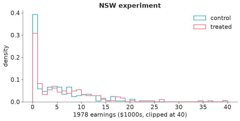
- A plot of the distribution of
re78in each experimental arm, and the numbers a likelihood would have to reproduce: share of exact zeros, median, mean, maximum. - A table showing whether randomisation balanced the pre-treatment covariates.
- One sentence: which textbook likelihoods are ruled out for
re78, and why?
COVARIATES = ["age", "educ", "black", "hisp", "marr", "nodegree", "re74", "re75"]
ARMS = ["control", "treated"]

fig, ax = plt.subplots(figsize=(8, 4))
bins = np.linspace(0, 40, 41)
for arm, grp in nsw.groupby("treat"):
    ax.hist(grp.re78.clip(upper=40_000) / 1000, bins=bins, histtype="step", lw=1.5, density=True, label=ARMS[arm])
ax.set(xlabel="1978 earnings ($1000s, clipped at 40)", ylabel="density", title="NSW experiment")
ax.legend()

nsw.groupby("treat").re78.agg(
    n="size", share_zero=lambda s: (s == 0).mean(), median="median", mean="mean", max="max"
).round(2)
| n | share_zero | median | mean | max | |
|---|---|---|---|---|---|
| treat | |||||
| 0 | 260 | 0.35 | 3138.80 | 4554.80 | 39483.53 |
| 1 | 185 | 0.24 | 4232.31 | 6349.14 | 60307.93 |
nsw.groupby("treat")[COVARIATES].mean().T.round(2)
| treat | 0 | 1 |
|---|---|---|
| age | 25.05 | 25.82 |
| educ | 10.09 | 10.35 |
| black | 0.83 | 0.84 |
| hisp | 0.11 | 0.06 |
| marr | 0.15 | 0.19 |
| nodegree | 0.83 | 0.71 |
| re74 | 2107.03 | 2095.57 |
| re75 | 1266.91 | 1532.06 |
A quarter to a third of the men earned exactly nothing in 1978 (35% of controls, 24% of the trained), the rest are strongly right-skewed, and one man earned $60,000. A Normal puts mass on negative earnings and no point mass at zero; Gamma and LogNormal cannot produce an exact zero at all. The outcome is really two outcomes: did he work? and how much did he earn if so?
The covariate means of the two arms agree closely, as randomisation promises (nodegree
differs a little - chance, with 445 people). Also note who these men are: average
pre-programme earnings of about $2,100 in 1974, and most of them earned nothing.
Task 1 · The experimental benchmark
Because of randomisation, the difference between the arms is the causal effect of training for men like these. Estimate it properly.
Deliver
- A Bayesian model of
re78by arm with the most obvious likelihood, and a posterior predictive check that shows specifically what it gets wrong. - A better likelihood, with priors you can defend on the dollar scale, clean diagnostics, and a posterior predictive check that passes where the first failed.
- The posterior of the average treatment effect in dollars (difference in mean earnings, zeros included), with a 94% interval and the probability that it exceeds $1,000 a year. This is the benchmark for everything that follows.
Solution
We work in thousands of dollars. First the model everyone writes: Normal earnings with a mean per arm.
warnings.filterwarnings("ignore", message=".*No safe default transform.*")  # HurdleGamma is a mixture; harmless here

t_exp = nsw.treat.values
y_exp = nsw.re78.values / 1000

with pm.Model(coords={"arm": ARMS}) as normal_model:
    mean = pm.Normal("mean", 5, 5, dims="arm")
    sigma = pm.HalfNormal("sigma", 10)
    pm.Deterministic("ate", mean[1] - mean[0])
    pm.Normal("re78", mean[t_exp], sigma, observed=y_exp)
    normal_idata = pm.sample(random_seed=RANDOM_SEED)
    pm.sample_posterior_predictive(normal_idata, extend_inferencedata=True, random_seed=RANDOM_SEED)

az.summary(normal_idata, var_names=["mean", "sigma", "ate"], ci_kind="hdi", ci_prob=0.94, round_to=2)
| mean | sd | hdi94_lb | hdi94_ub | ess_bulk | ess_tail | r_hat | mcse_mean | mcse_sd | |
|---|---|---|---|---|---|---|---|---|---|
| mean[control] | 4.56 | 0.40 | 3.81 | 5.30 | 6192.29 | 3155.98 | 1.0 | 0.01 | 0.01 |
| mean[treated] | 6.34 | 0.49 | 5.42 | 7.23 | 6259.56 | 3120.36 | 1.0 | 0.01 | 0.01 |
| sigma | 6.59 | 0.22 | 6.19 | 7.01 | 6386.21 | 3503.90 | 1.0 | 0.00 | 0.00 |
| ate | 1.78 | 0.63 | 0.55 | 2.92 | 6200.97 | 3170.18 | 1.0 | 0.01 | 0.01 |
A hurdle model matches the two-part story from Task 0: with probability $\psi$ a man has positive earnings, and if so they are Gamma distributed with mean $\mu$. Mean earnings including the zeros are then $\psi\mu$, and the ATE is the difference of that product between arms.
Priors, on the $1000 scale: a full-time minimum-wage job paid about $5,500 a year in 1978,
and these are men on the margins of the labour market, so Gamma(mu=8, sigma=5) for mean
positive earnings covers roughly 1.5 to 19. Beta(2, 2) on $\psi$ says only "not 0, not 1".
The prior predictive check below turns those into an implied prior on the ATE.
with pm.Model(coords={"arm": ARMS}) as hurdle_model:
    psi = pm.Beta("psi", 2, 2, dims="arm")
    mu_pos = pm.Gamma("mu_pos", mu=8, sigma=5, dims="arm")
    shape = pm.Gamma("shape", mu=1.5, sigma=1)
    mean = pm.Deterministic("mean", psi * mu_pos, dims="arm")
    pm.Deterministic("ate", mean[1] - mean[0])
    pm.HurdleGamma("re78", psi=psi[t_exp], alpha=shape, beta=shape / mu_pos[t_exp], observed=y_exp)
    hurdle_prior = pm.sample_prior_predictive(1000, random_seed=RANDOM_SEED)

prior_ate = hurdle_prior.prior["ate"].values.ravel()
print("prior 94% interval for the ATE ($1000s):", np.quantile(prior_ate, [0.03, 0.97]).round(1))
print("prior 94% interval for mean earnings   :", np.quantile(hurdle_prior.prior["mean"].values, [0.03, 0.97]).round(1))
prior 94% interval for the ATE ($1000s): [-9.6  8.6]
prior 94% interval for mean earnings   : [ 0.4 11.6]
with hurdle_model:
    hurdle_idata = pm.sample(random_seed=RANDOM_SEED)
    pm.sample_posterior_predictive(hurdle_idata, extend_inferencedata=True, random_seed=RANDOM_SEED)

print("divergences:", int(hurdle_idata.sample_stats["diverging"].sum()))
az.summary(hurdle_idata, ci_kind="hdi", ci_prob=0.94, round_to=2)
divergences: 0
| mean | sd | hdi94_lb | hdi94_ub | ess_bulk | ess_tail | r_hat | mcse_mean | mcse_sd | |
|---|---|---|---|---|---|---|---|---|---|
| psi[control] | 0.64 | 0.03 | 0.59 | 0.70 | 6121.91 | 3539.34 | 1.0 | 0.00 | 0.00 |
| psi[treated] | 0.75 | 0.03 | 0.69 | 0.81 | 6178.58 | 3042.08 | 1.0 | 0.00 | 0.00 |
| mu_pos[control] | 7.08 | 0.46 | 6.23 | 7.93 | 6285.15 | 3172.72 | 1.0 | 0.01 | 0.01 |
| mu_pos[treated] | 8.41 | 0.60 | 7.30 | 9.47 | 6367.59 | 3447.37 | 1.0 | 0.01 | 0.01 |
| shape | 1.42 | 0.10 | 1.22 | 1.61 | 5963.90 | 3563.19 | 1.0 | 0.00 | 0.00 |
| mean[control] | 4.56 | 0.36 | 3.91 | 5.23 | 6187.43 | 3488.66 | 1.0 | 0.00 | 0.01 |
| mean[treated] | 6.32 | 0.52 | 5.37 | 7.31 | 6636.87 | 3136.63 | 1.0 | 0.01 | 0.01 |
| ate | 1.76 | 0.64 | 0.66 | 3.06 | 6935.91 | 3041.33 | 1.0 | 0.01 | 0.01 |
def ppc_panel(ax, idata, title):
    """Replicated histograms against the observed one, plus the two statistics that matter."""
    rep = az.extract(idata, group="posterior_predictive", var_names="re78", num_samples=200, random_seed=RANDOM_SEED)
    rep = rep.values.T  # (draws, obs)
    bins = np.linspace(-15, 40, 56)
    for r in rep[:40]:
        ax.hist(r, bins=bins, histtype="step", color="C0", alpha=0.15)
    ax.hist(y_exp, bins=bins, histtype="step", color="k", lw=1.5, label="observed")
    ax.set(xlabel="1978 earnings ($1000s)", title=title)
    ax.legend()
    print(
        f"{title:<14} zeros: observed {np.mean(y_exp == 0):.2f}, replicated {np.mean(rep == 0):.2f} | "
        f"negative: replicated {np.mean(rep < 0):.2f} | "
        f"99th pct: observed {np.quantile(y_exp, 0.99):.1f}, replicated {np.quantile(rep, 0.99):.1f}"
    )


fig, axes = plt.subplots(1, 2, figsize=(11, 4), sharey=True)
ppc_panel(axes[0], normal_idata, "Normal")
ppc_panel(axes[1], hurdle_idata, "Hurdle-Gamma")
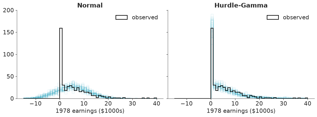
Normal         zeros: observed 0.31, replicated 0.00 | negative: replicated 0.21 | 99th pct: observed 26.6, replicated 20.8
Hurdle-Gamma   zeros: observed 0.31, replicated 0.31 | negative: replicated 0.00 | 99th pct: observed 26.6, replicated 28.7
ate_exp = hurdle_idata.posterior["ate"]  # $1000s
print(f"experimental ATE: ${1000 * float(ate_exp.mean()):,.0f}")
print("94% interval ($):", (1000 * np.quantile(ate_exp, [0.03, 0.97])).round(0))
print(f"P(ATE > $1,000) = {float((ate_exp > 1).mean()):.2f}")
print(f"raw difference in means: ${1000 * (y_exp[t_exp == 1].mean() - y_exp[t_exp == 0].mean()):,.0f}")
experimental ATE: $1,762
94% interval ($): [ 598. 3004.]
P(ATE > $1,000) = 0.89
raw difference in means: $1,794
assert h.check("task1", ate=1000 * ate_exp.mean(), p_ate_gt_1000=(ate_exp > 1).mean())
- PASS
ate= 1762 is consistent with the reference solution. - PASS
p_ate_gt_1000= 0.89 is consistent with the reference solution.
The Normal model predicts that about a fifth of the men earn negative amounts and nobody earns exactly zero; the hurdle model reproduces the 31% of zeros and the right tail. Both give nearly the same ATE, because a difference in means is robust to the likelihood - but only the hurdle model tells the ministry how training works: about half of the effect is more men in work ($\psi$ rises from 0.64 to 0.75) and half is higher earnings among those who work (from about $7,100 to $8,400).
The benchmark: training raised 1978 earnings by about $1,750, 94% interval roughly $600 to $3,000, and the probability that the effect exceeds $1,000 is about 0.89. Because assignment was random this is also the effect on the treated (the ATT), which is what the observational analysis below can hope to estimate.
Task 2 · The ministry's dataset
Now forget the experimental controls. The ministry has the 185 participants and the CPS.
Deliver
- The observational dataset (NSW treated + all CPS men) and the naive estimate: the difference in mean 1978 earnings between participants and non-participants.
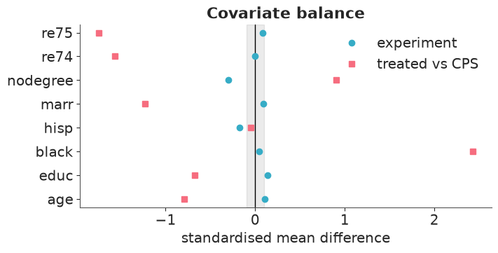
- A covariate balance table - means by group and standardised mean differences - side by side with the same table for the experiment.
- A short paragraph for the ministry explaining why the naive number says nothing about the programme. Look closely at the CPS earnings columns too: is there anything about how they were recorded that a model should know?
treated = nsw[nsw.treat == 1]
obs = pd.concat([treated, cps], ignore_index=True)

naive = obs.re78[obs.treat == 1].mean() - obs.re78[obs.treat == 0].mean()
print(f"naive difference in means: ${naive:,.0f}")


def smd(a, b):
    """Standardised mean difference: (mean_a - mean_b) / pooled sd."""
    return (a.mean() - b.mean()) / np.sqrt((a.var() + b.var()) / 2)


exp_controls = nsw[nsw.treat == 0]
balance = pd.DataFrame(
    {
        "NSW treated": treated[COVARIATES].mean(),
        "NSW controls": exp_controls[COVARIATES].mean(),
        "CPS": cps[COVARIATES].mean(),
        "SMD vs NSW controls": [smd(treated[c], exp_controls[c]) for c in COVARIATES],
        "SMD vs CPS": [smd(treated[c], cps[c]) for c in COVARIATES],
    }
)
balance.round(2)
naive difference in means: $-8,498
| NSW treated | NSW controls | CPS | SMD vs NSW controls | SMD vs CPS | |
|---|---|---|---|---|---|
| age | 25.82 | 25.05 | 33.23 | 0.11 | -0.80 |
| educ | 10.35 | 10.09 | 12.03 | 0.14 | -0.68 |
| black | 0.84 | 0.83 | 0.07 | 0.04 | 2.43 |
| hisp | 0.06 | 0.11 | 0.07 | -0.17 | -0.05 |
| marr | 0.19 | 0.15 | 0.71 | 0.09 | -1.23 |
| nodegree | 0.71 | 0.83 | 0.30 | -0.30 | 0.90 |
| re74 | 2095.57 | 2107.03 | 14016.80 | -0.00 | -1.57 |
| re75 | 1532.06 | 1266.91 | 13650.80 | 0.08 | -1.75 |
fig, ax = plt.subplots(figsize=(7, 3.5))
ax.axvline(0, color="k", lw=1)
ax.axvspan(-0.1, 0.1, color="k", alpha=0.08)
ax.plot(balance["SMD vs NSW controls"], COVARIATES, "o", label="experiment")
ax.plot(balance["SMD vs CPS"], COVARIATES, "s", label="treated vs CPS")
ax.set(xlabel="standardised mean difference", title="Covariate balance")
ax.legend();
profile = lambda d: (d.black == 1) & (d.marr == 0) & (d.re74 == 0) & (d.re75 == 0)
print(f"Black, unmarried, no earnings in 1974 or 1975: {profile(treated).sum()} of {len(treated)} participants, "
      f"{profile(cps).sum()} of {len(cps):,} CPS men")
for col in ["re74", "re75", "re78"]:
    top = cps[col].max()
    print(f"CPS {col}: max {top:,.0f}, share exactly at the max {np.mean(cps[col] == top):.2f}")
Black, unmarried, no earnings in 1974 or 1975: 81 of 185 participants, 58 of 15,992 CPS men
CPS re74: max 25,862, share exactly at the max 0.19
CPS re75: max 25,244, share exactly at the max 0.19
CPS re78: max 25,565, share exactly at the max 0.26
assert h.check("task2", naive_diff=naive, smd_black=balance.loc["black", "SMD vs CPS"])
- PASS
naive_diff= -8498 is consistent with the reference solution. - PASS
smd_black= 2.428 is consistent with the reference solution.
The naive comparison says training costs a man $8,500 a year. It is a comparison of two different populations. Rule of thumb: an SMD beyond ±0.1 is worth worrying about. The experiment stays inside ±0.3; against the CPS, *every* covariate except `hisp` is off by 0.7 to 2.4 standard deviations. Participants are 84% Black (CPS: 7%), 19% married (71%), and earned $2,100 in 1974 against $14,000. The programme selected men with poor earnings prospects, so they would have earned less than the average CPS man in 1978 with or without training. Only 58 of the 15,992 CPS men share the most common participant profile.
Two more things a careful analyst notices. CPS earnings are top-coded: a quarter of CPS men sit exactly at $25,565 in 1978 (and a fifth at the cap in 1974-75), so the CPS outcome is censored where the participants are not. And the two groups' earnings come from different sources (programme records versus a household survey). Neither problem can be fixed by regression; both matter less the more we restrict attention to low-earning CPS men.
Task 3 · A causal model, conditioned and intervened on
Deliver
- The causal DAG you are assuming, drawn in a markdown cell, with the adjustment set it implies and the assumptions that are not testable from these data.
- One generative PyMC model of the observational data - treatment assignment and
1978 earnings given the covariates - written without any observed data. Condition it on
the data with
pm.observe, fit it, and then usepm.doto settreatto 0 and to 1 for the participants. From those two interventions compute the posterior of the ATT (average effect on the 185 participants) by g-computation. - Compare with the benchmark. How far off is it, and in which direction?
Use all 16,177 rows here. Sampling takes around a minute; storing a 16,177-long deterministic for every draw is what you need to avoid.
Solution
            X = {age, educ, black, hisp, marr, nodegree, re74, re75}
             │                                   │
             ▼                                   ▼
          treat  ───────────────────────────►  re78
             ▲                                   ▲
             └ ─ ─ ─ ─ ─ ─ ─   U   ─ ─ ─ ─ ─ ─ ─ ┘
                (motivation, health, local labour market, ...)
Every covariate is measured before treatment, plausibly affects both who ends up in the
programme and what they earn later, and cannot be affected by the programme. Conditioning
on all of $X$ closes every back-door path treat ← X → re78, so the adjustment set is all
eight covariates. Pre-programme earnings do the heavy lifting: they are the best available
proxy for the unobservables $U$.
Untestable assumptions: (1) no unmeasured confounding - the dashed $U$ paths are absent once we condition on $X$; (2) positivity - for every kind of participant there are comparable non-participants (we will test this one in Task 4, and it fails); (3) the outcome means the same thing in both data sources.
The generative model has two parts: a logistic model for who gets treated and the hurdle-Gamma earnings model from Task 1, now with covariates and a treatment effect on both the probability of working and the level of earnings. Writing it as a function of a data frame means the same code describes any population we want to intervene on.
def features(df, names):
    """Design matrix on scales where Normal(0, 1) priors are weakly informative."""
    d = pd.DataFrame(index=df.index)
    d["age"] = (df.age - 30) / 10
    d["educ"] = (df.educ - 11) / 3
    for col in ["black", "hisp", "marr", "nodegree"]:
        d[col] = df[col].astype(float)
    d["re74"] = df.re74 / 10_000
    d["re75"] = df.re75 / 10_000
    d["age2"] = d.age**2
    d["u74"] = (df.re74 == 0).astype(float)  # no earnings at all in 1974
    d["u75"] = (df.re75 == 0).astype(float)
    return d[list(names)]


def generative(df, names):
    """Generative model of (treat, re78) given covariates. Nothing is observed yet."""
    X = features(df, names).values
    with pm.Model(coords={"obs": df.index.values, "cov": list(names)}) as gen:
        # who gets treated
        g0 = pm.Normal("g0", 0, 3)
        g = pm.Normal("g", 0, 2, dims="cov")
        treat = pm.Bernoulli("treat", logit_p=g0 + pm.math.dot(X, g), dims="obs")
        # what they earn: P(any earnings) and mean earnings if positive ($1000s)
        a_z = pm.Normal("a_z", 0, 2)
        b_z = pm.Normal("b_z", 0, 1, dims="cov")
        tau_z = pm.Normal("tau_z", 0, 1)
        a_m = pm.Normal("a_m", 2, 1)
        b_m = pm.Normal("b_m", 0, 1, dims="cov")
        tau_m = pm.Normal("tau_m", 0, 1)
        shape = pm.Gamma("shape", mu=1.5, sigma=1)
        psi = pm.math.sigmoid(a_z + tau_z * treat + pm.math.dot(X, b_z))
        mu = pm.math.exp(a_m + tau_m * treat + pm.math.dot(X, b_m))
        pm.Deterministic("expected", psi * mu, dims="obs")  # E[re78 | treat, X]
        pm.HurdleGamma("re78", psi=psi, alpha=shape, beta=shape / mu, dims="obs")
    return gen


PARAMETERS = ["g0", "g", "a_z", "b_z", "tau_z", "a_m", "b_m", "tau_m", "shape"]
logging.getLogger("pymc.sampling.forward").setLevel(logging.WARNING)  # silence "Sampling: []" below


def fit(df, names):
    """Condition the generative model on the data and sample. Only parameters are stored."""
    conditioned = pm.observe(generative(df, names), {"treat": df.treat.values, "re78": df.re78.values / 1000})
    with conditioned:
        idata = pm.sample(var_names=PARAMETERS, nuts_sampler="nutpie", random_seed=RANDOM_SEED)
    worst = az.summary(idata)
    print(f"n = {len(df):,}: divergences {int(idata.sample_stats['diverging'].sum())}, "
          f"max r_hat {worst.r_hat.max():.3f}, min ESS {worst.ess_bulk.min():.0f}")
    return idata


def expected_under(idata, df, names, treat_value):
    """Posterior of E[re78 | do(treat = treat_value), X_i] for every row of df."""
    intervened = pm.do(generative(df, names), {"treat": np.full(len(df), treat_value)})
    with intervened:
        pp = pm.sample_posterior_predictive(
            idata, var_names=["expected"], random_seed=RANDOM_SEED, progressbar=False
        )
    return pp.posterior_predictive["expected"]


def att(idata, names):
    """g-computation: average over the participants of E[Y | do(1), X] - E[Y | do(0), X]."""
    return (expected_under(idata, treated, names, 1) - expected_under(idata, treated, names, 0)).mean("obs")


def describe(label, draws):
    v = 1000 * np.asarray(draws).ravel()
    lo, hi = np.quantile(v, [0.03, 0.97])
    return {"analysis": label, "mean": v.mean(), "sd": v.std(), "lo94": lo, "hi94": hi, "P(>$1,000)": np.mean(v > 1000)}
pm.observe turns the named random variables into observed ones; pm.do replaces a random
variable by a constant, cutting the arrow from $X$ into treat. Because pm.do is applied
to the generative model built on the participants' rows, sampling expected from it
with the fitted posterior gives the participants' potential outcomes directly.
The first attempt adjusts linearly (on the link scales) for the eight covariates.
BASE = COVARIATES
full_idata = fit(obs, BASE)
att_full = att(full_idata, BASE)

results = [describe("experiment (benchmark)", ate_exp), describe("full CPS, linear adjustment", att_full)]
pd.DataFrame(results).set_index("analysis").round({"mean": 0, "sd": 0, "lo94": 0, "hi94": 0, "P(>$1,000)": 2})
n = 16,177: divergences 0, max r_hat 1.006, min ESS 2088
| mean | sd | lo94 | hi94 | P(>$1,000) | |
|---|---|---|---|---|---|
| analysis | |||||
| experiment (benchmark) | 1762.0 | 638.0 | 598.0 | 3004.0 | 0.89 |
| full CPS, linear adjustment | 74.0 | 432.0 | -707.0 | 897.0 | 0.02 |
assert h.check("task3", att_full=1000 * att_full.mean())
- PASS
att_full= 73.67 is consistent with the reference solution.
Regression adjustment has moved the estimate from −$8,500 to about **zero** - an
improvement of eight thousand dollars, and still the wrong answer: the model is confident
(sd about $430) that the effect is below $1,000, while the experiment says it is probably
above. The sampler is perfectly happy. Nothing in r_hat or ESS can tell you that a causal
estimate is wrong.
Task 4 · Where do the counterfactuals come from?
The ATT needs, for each participant, a prediction of what he would have earned without training. Those predictions are only as good as the non-participants who resemble him.
Deliver
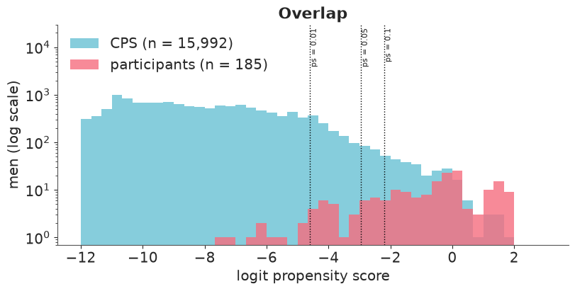
- A diagnosis: estimate every man's probability of being a participant given his covariates (the propensity score - you may already have it) and compare its distribution in the two groups. What share of the CPS has a propensity below 1%?
- Evidence, not using the experimental controls, that the Task 3 outcome model is wrong in the region of covariate space where the participants live.
- A fix, a refit with clean diagnostics, and the new ATT next to the benchmark. State exactly which population your new estimate refers to.
Solution
The treatment part of the generative model is a propensity model, and it was fitted along with everything else. To give it a fair chance of separating the groups we use a richer covariate set from here on: a quadratic in age and indicators for zero earnings in 1974 and 1975 (being out of work is qualitatively different from earning little).
FLEX = BASE + ["age2", "u74", "u75"]
flex_idata = fit(obs, FLEX)
att_flex = att(flex_idata, FLEX)


def propensity(idata, df, names):
    post = az.extract(idata, var_names=["g0", "g"], num_samples=400, random_seed=RANDOM_SEED)
    logit = post["g0"].values[None, :] + features(df, names).values @ post["g"].transpose("cov", "sample").values
    return expit(logit).mean(axis=1)


obs["ps"] = propensity(flex_idata, obs, FLEX)
is_treated = obs.treat == 1

fig, ax = plt.subplots(figsize=(8, 4))
bins = np.linspace(-12, 3, 46)
logit_ps = np.log(obs.ps / (1 - obs.ps))
ax.hist(logit_ps[~is_treated], bins=bins, alpha=0.6, label=f"CPS (n = {(~is_treated).sum():,})")
ax.hist(logit_ps[is_treated], bins=bins, alpha=0.8, label=f"participants (n = {is_treated.sum()})")
for p in (0.01, 0.05, 0.1):
    ax.axvline(np.log(p / (1 - p)), color="k", ls=":", lw=1)
    ax.text(np.log(p / (1 - p)), 25_000, f" ps = {p:g}", rotation=90, va="top", fontsize=8)
ax.set(yscale="log", ylim=(0.7, 30_000), xlabel="logit propensity score", ylabel="men (log scale)", title="Overlap")
ax.legend(loc="upper left");
n = 16,177: divergences 0, max r_hat 1.003, min ESS 1623
share_below = np.mean(obs.ps[~is_treated] < 0.01)
print(f"share of CPS men with propensity below 1%: {share_below:.3f}")
overlap = pd.DataFrame(
    {
        "CPS kept": [int(((obs.ps >= p) & ~is_treated).sum()) for p in (0.01, 0.05, 0.1)],
        "participants above": [int(((obs.ps >= p) & is_treated).sum()) for p in (0.01, 0.05, 0.1)],
    },
    index=pd.Index([0.01, 0.05, 0.1], name="propensity >="),
)
print(f"propensity above 0.5: {((obs.ps > 0.5) & is_treated).sum()} participants, "
      f"{((obs.ps > 0.5) & ~is_treated).sum()} CPS men")
overlap
share of CPS men with propensity below 1%: 0.913
propensity above 0.5: 66 participants, 30 CPS men
| CPS kept | participants above | |
|---|---|---|
| propensity >= | ||
| 0.01 | 1393 | 175 |
| 0.05 | 404 | 157 |
| 0.10 | 256 | 142 |
More than nine CPS men in ten have less than a 1% chance of being a participant: they are older, married, steadily employed men who tell us nothing about the counterfactual of an unemployed 25-year-old. Yet they are 90% of the likelihood, so they decide the regression coefficients, and the participants' counterfactuals are an extrapolation of a curve fitted elsewhere.
That can be checked without the experiment. If the outcome model is right, it should predict the 1978 earnings of the few CPS men who do look like participants:
lookalikes = obs[(obs.ps >= 0.05) & ~is_treated]
print(f"{len(lookalikes)} CPS look-alikes earned ${lookalikes.re78.mean():,.0f} on average in 1978 "
      f"(standard error ${lookalikes.re78.std() / np.sqrt(len(lookalikes)):,.0f})")
for label, idata, names in [("linear", full_idata, BASE), ("flexible", flex_idata, FLEX)]:
    pred = expected_under(idata, lookalikes, names, 0).mean("obs")
    print(f"{label:>9} full-sample model predicts ${1000 * float(pred.mean()):,.0f} for them "
          f"(94% interval {(1000 * np.quantile(pred, [0.03, 0.97])).round(0)})")
404 CPS look-alikes earned $5,666 on average in 1978 (standard error $324)
   linear full-sample model predicts $6,682 for them (94% interval [6389. 6981.])
flexible full-sample model predicts $6,384 for them (94% interval [6085. 6689.])
The fix is to stop asking the model to extrapolate: keep all participants (so the estimand stays the ATT for the 185 men) but only those CPS men with a propensity of at least 5%, and refit the same generative model on that common-support sample.
def trimmed(threshold):
    return obs[(obs.ps >= threshold) | is_treated]


trim_df = trimmed(0.05)
print(f"controls kept: {(trim_df.treat == 0).sum()}, "
      f"of which top-coded: {np.mean(trim_df.re78[trim_df.treat == 0] >= cps.re78.max()):.3f}")
balance_trim = pd.DataFrame(
    {
        "SMD vs all CPS": balance["SMD vs CPS"],
        "SMD vs trimmed CPS": [smd(treated[c], trim_df.loc[trim_df.treat == 0, c]) for c in COVARIATES],
    }
)
balance_trim.round(2)
controls kept: 404, of which top-coded: 0.007
| SMD vs all CPS | SMD vs trimmed CPS | |
|---|---|---|
| age | -0.80 | -0.00 |
| educ | -0.68 | -0.03 |
| black | 2.43 | -0.09 |
| hisp | -0.05 | -0.14 |
| marr | -1.23 | -0.13 |
| nodegree | 0.90 | 0.18 |
| re74 | -1.57 | -0.24 |
| re75 | -1.75 | -0.19 |
trim_idata = fit(trim_df, FLEX)
att_trim = att(trim_idata, FLEX)

results += [describe("full CPS, flexible adjustment", att_flex), describe("trimmed (ps >= 0.05), flexible", att_trim)]
pd.DataFrame(results).set_index("analysis").round({"mean": 0, "sd": 0, "lo94": 0, "hi94": 0, "P(>$1,000)": 2})
n = 589: divergences 0, max r_hat 1.002, min ESS 1735
| mean | sd | lo94 | hi94 | P(>$1,000) | |
|---|---|---|---|---|---|
| analysis | |||||
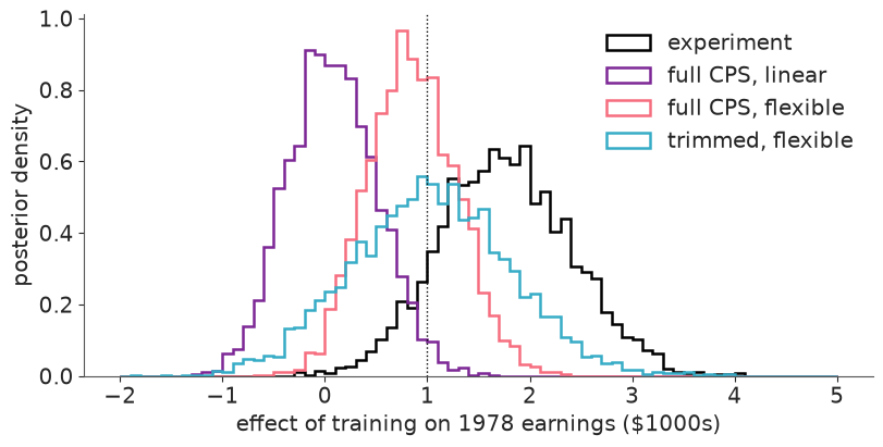
| experiment (benchmark) | 1762.0 | 638.0 | 598.0 | 3004.0 | 0.89 |
| full CPS, linear adjustment | 74.0 | 432.0 | -707.0 | 897.0 | 0.02 |
| full CPS, flexible adjustment | 851.0 | 435.0 | 70.0 | 1673.0 | 0.36 |
| trimmed (ps >= 0.05), flexible | 1030.0 | 773.0 | -371.0 | 2467.0 | 0.51 |
fig, ax = plt.subplots(figsize=(8, 4))
bins = np.linspace(-2, 5, 71)
for label, draws, color in [
    ("experiment", ate_exp, "k"),
    ("full CPS, linear", att_full, "C3"),
    ("full CPS, flexible", att_flex, "C1"),
    ("trimmed, flexible", att_trim, "C0"),
]:
    ax.hist(np.asarray(draws).ravel(), bins=bins, histtype="step", lw=1.8, density=True, color=color, label=label)
ax.axvline(1, color="k", ls=":", lw=1)
ax.set(xlabel="effect of training on 1978 earnings ($1000s)", ylabel="posterior density")
ax.legend();
assert h.check("task4", cps_share_below_1pct=share_below, att_trimmed=1000 * att_trim.mean())
- PASS
cps_share_below_1pct= 0.9129 is consistent with the reference solution. - PASS
att_trimmed= 1030 is consistent with the reference solution.
Both full-sample models over-predict what the look-alike CPS men earned by $700 to $1,000, two to three standard errors of that average: the fit is dominated by men elsewhere in covariate space. Over-predicting the untreated outcome of men like the participants is exactly what biases the ATT downwards.
After trimming, 404 of the 15,992 CPS men remain. Every SMD is now within ±0.25 (it was up to 2.4), and fewer than 1% of the remaining controls are top-coded, so that problem has gone too. The estimates move in the right direction at each step - about $70 with the linear full-sample model, $850 once age squared and the zero-earnings indicators are added, $1,030 on the common-support sample - and the posterior sd almost doubles, from $430 to $770. That is the honest price: the full-sample posterior was narrow because 15,000 irrelevant men were voting.
The benchmark of $1,760 sits comfortably inside the trimmed model's 94% interval (about −$370 to $2,470), but the point estimate is still $700 short of it, and zero is inside the interval too. The estimand is unchanged - the ATT for all 185 participants - but 28 of them have a propensity below 0.05 and therefore few close comparisons, and at the other end (propensity above one half) participants outnumber the CPS men they are compared with. For those men the model is still doing more work than the data.
Task 5 · How fragile is the answer?
You made choices in Task 4 that the ministry cannot audit. Show what they are worth.
Deliver a table and a plot of the ATT posterior under
- at least three trimming thresholds, and
- at least three adjustment sets on your preferred trimmed sample: all covariates, without
re74, and without any pre-programme earnings.
Then answer: which choice matters most, and what does that say about the DAG in Task 3?
NO_RE74 = [c for c in FLEX if c not in ("re74", "u74")]
NO_EARNINGS = [c for c in NO_RE74 if c not in ("re75", "u75")]

sensitivity = {"ps >= 0.05, all covariates": att_trim}
for label, threshold, names in [
    ("ps >= 0.01, all covariates", 0.01, FLEX),
    ("ps >= 0.10, all covariates", 0.10, FLEX),
    ("ps >= 0.05, without re74", 0.05, NO_RE74),
    ("ps >= 0.05, without re74 and re75", 0.05, NO_EARNINGS),
]:
    sensitivity[label] = att(fit(trimmed(threshold), names), names)

sens_table = pd.DataFrame([describe(k, v) for k, v in sensitivity.items()]).set_index("analysis")
sens_table.round({"mean": 0, "sd": 0, "lo94": 0, "hi94": 0, "P(>$1,000)": 2})
n = 1,578: divergences 0, max r_hat 1.004, min ESS 1433
n = 441: divergences 0, max r_hat 1.003, min ESS 1477
n = 589: divergences 0, max r_hat 1.004, min ESS 1363
n = 589: divergences 0, max r_hat 1.003, min ESS 1258
| mean | sd | lo94 | hi94 | P(>$1,000) | |
|---|---|---|---|---|---|
| analysis | |||||
| ps >= 0.05, all covariates | 1030.0 | 773.0 | -371.0 | 2467.0 | 0.51 |
| ps >= 0.01, all covariates | 1118.0 | 650.0 | -30.0 | 2348.0 | 0.57 |
| ps >= 0.10, all covariates | 1376.0 | 857.0 | -204.0 | 3031.0 | 0.66 |
| ps >= 0.05, without re74 | 1090.0 | 715.0 | -201.0 | 2469.0 | 0.55 |
| ps >= 0.05, without re74 and re75 | 235.0 | 723.0 | -1090.0 | 1673.0 | 0.14 |
fig, ax = plt.subplots(figsize=(9, 3.8))
rows = pd.concat([pd.DataFrame([describe("experiment (benchmark)", ate_exp)]).set_index("analysis"), sens_table])[::-1]
ypos = np.arange(len(rows))
ax.errorbar(rows["mean"], ypos, xerr=[rows["mean"] - rows["lo94"], rows["hi94"] - rows["mean"]], fmt="o", capsize=3)
ax.axvline(1000, color="k", ls=":", lw=1)
ax.axvline(0, color="k", lw=1)
ax.set_yticks(ypos, rows.index)
ax.set(xlabel="effect on 1978 earnings ($)", title="Posterior mean and 94% interval");
assert h.check("task5", att_no_earnings=1000 * sensitivity["ps >= 0.05, without re74 and re75"].mean())
- PASS
att_no_earnings= 235.4 is consistent with the reference solution.
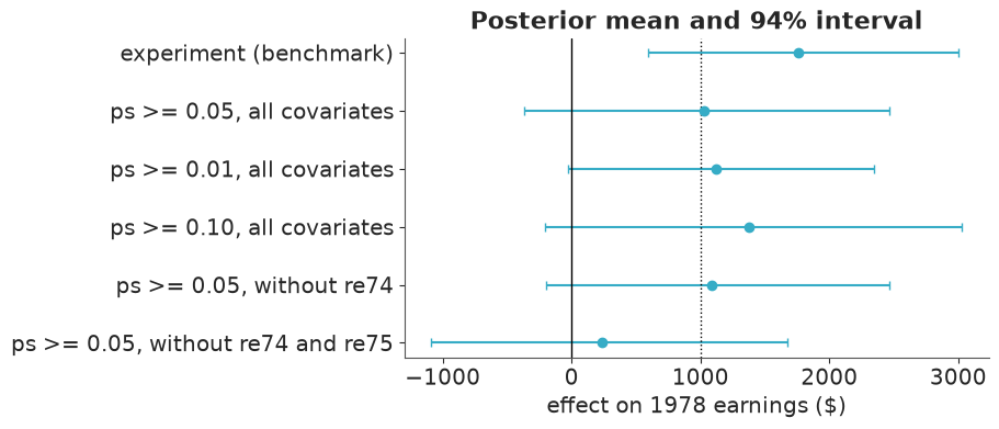
Trimming threshold. Between 0.01 and 0.10 the posterior mean moves from about $1,030 to $1,380, much less than one posterior sd ($650 to $860). Every interval contains the benchmark and every interval contains zero. Tighter trimming trades bias for variance, as it should.
Adjustment set. Dropping re74 alone changes nothing ($1,090): given `re75`, and given
a sample that was itself selected with a propensity score that knew `re74`, it carries
little extra information here. Dropping *both* years of earnings cuts the estimate to
about $240 and $P(\text{effect} > \$1{,}000)$ from roughly 0.5 to 0.14 - and this
understates their importance, because the trimmed sample was still chosen using them.
So what we adjust for matters more than how we trim. That is a statement about the DAG:
the whole analysis rests on having measured the confounders, and the one time we can test
that - by hiding a confounder we do have - the answer moves by $800. Nothing in the data
says re75 was the last such variable; programme applicants typically enrol just after
their earnings have dipped, and two years of history may not capture that.
Task 6 · What do you tell the ministry?
The ministry's economists say the programme pays for itself if it raises participants' earnings by more than $1,000 a year (an illustrative threshold).
Deliver
- $P(\text{effect} > \$1{,}000)$ under the experiment, under the naive full-sample adjustment, and under your preferred observational analysis.
- A short note to the ministry: what the observational data can and cannot support, what you would need to see before trusting an observational answer when there is no experiment to check it against, and whether the memo closing the programme should go out.
decision = pd.DataFrame(
    [
        describe("experiment (benchmark)", ate_exp),
        describe("observational: full CPS, linear", att_full),
        describe("observational: full CPS, flexible", att_flex),
        describe("observational: trimmed, flexible", att_trim),
    ]
).set_index("analysis")
decision.round({"mean": 0, "sd": 0, "lo94": 0, "hi94": 0, "P(>$1,000)": 2})
| mean | sd | lo94 | hi94 | P(>$1,000) | |
|---|---|---|---|---|---|
| analysis | |||||
| experiment (benchmark) | 1762.0 | 638.0 | 598.0 | 3004.0 | 0.89 |
| observational: full CPS, linear | 74.0 | 432.0 | -707.0 | 897.0 | 0.02 |
| observational: full CPS, flexible | 851.0 | 435.0 | 70.0 | 1673.0 | 0.36 |
| observational: trimmed, flexible | 1030.0 | 773.0 | -371.0 | 2467.0 | 0.51 |
assert h.check("task6", p_observational=float((att_trim > 1).mean()))
- PASS
p_observational= 0.514 is consistent with the reference solution.
Note to the ministry
- Do not send the memo. The −$8,500 gap is a comparison of unemployed, mostly unmarried 25-year-olds with the average American working man. It says nothing about the programme.
- *Our best observational estimate is about +$1,000 a year* (94% interval roughly −$400 to +$2,500). The probability that the programme clears the $1,000 bar is about one half on this evidence. The experiment puts it at 0.89, with an estimate of about $1,760. The observational analysis gets the sign right and its interval covers the experimental answer, but its point estimate is some 40% too low, and we only know that because the experiment exists.
- The dangerous analysis is the respectable-looking one. Regression on all 16,000 CPS men gave a tight interval around zero, $P = 0.02$, and flawless sampler diagnostics. It was confidently wrong, because nine in ten of those men could never have been participants and the model extrapolated from them.
- None of these intervals includes the uncertainty that matters most - whether we measured everything that drove both enrolment and earnings. Removing pre-programme earnings moved the answer by more than any modelling choice did.
Before trusting an observational estimate with no experiment behind it, ask for: overlap and post-trimming balance; a predictive check of the outcome model on look-alike controls (Task 4); stability across reasonable thresholds and adjustment sets (Task 5); a placebo test, such as the "effect" of training on 1975 earnings, which must be zero; and an explicit statement of how strong an unmeasured confounder would have to be to overturn the decision. Better still, randomise a pilot.
Going further
- Respect the top-coding. A quarter of CPS men have
re78recorded at the cap. Model that explicitly with a censored likelihood for positive earnings (you will have to split the hurdle into its two parts to do it). Does the full-sample estimate move? Does the trimmed one? - Weight instead of trim. Use the propensity scores to weight CPS men by
$e(x) / (1 - e(x))$ in the outcome likelihood (
pm.Potential), or combine weighting and outcome modelling into a doubly-robust estimate. Propagate the uncertainty in $e(x)$. - A more flexible response surface. Replace the linear predictors by an HSGP or BART-like
additive model in
re74,re75andage. Does flexibility substitute for trimming, or only hide the extrapolation? - Unmeasured confounding. Add a sensitivity parameter: a latent binary $U$ that raises both the odds of participation and earnings. How strong must it be to push $P(\text{effect} > \$1{,}000)$ below one half?
h.progress()
C09: 0/20 hints used, 9/9 checks passed.