E01 · The Bayesian workflow in PyMC 6 — Bayesian Modelling in Practice

Every challenge in this repository assumes you can do what is on this page without thinking. It is also a tour of what changed if you learned PyMC a few versions ago:

Then	Now (PyMC 6 / ArviZ 1)
`pm.sample` returns `InferenceData`	returns an xarray `DataTree`; groups work the same (`idata.posterior["x"]`)
`pm.MutableData`, `pm.ConstantData`	just `pm.Data`
`az.plot_posterior`, `az.plot_ppc`	`az.plot_dist`, `az.plot_ppc_dist` (and a family of `plot_ppc_*`)
`az.summary` shows 94% HDI	shows an 89% equal-tailed interval by default; ask for what you want with `ci_kind=`, `ci_prob=`
plots return matplotlib axes	plots return a `PlotCollection`
`pm.sample` uses PyMC's NUTS	uses nutpie automatically when it is installed

import arviz as az
import matplotlib.pyplot as plt
import numpy as np
import pandas as pd
import pymc as pm

from pymc_challenges import data

RANDOM_SEED = 42
rng = np.random.default_rng(RANDOM_SEED)
az.style.use("arviz-variat")

print(f"PyMC {pm.__version__}, ArviZ {az.__version__}")

PyMC 6.3.2, ArviZ 1.3.0

1 · Question and data

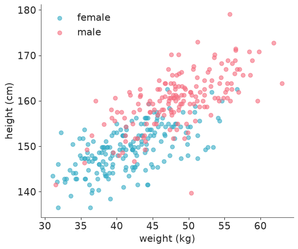
How does height depend on weight among adults, and does it differ by sex? A deliberately simple question, so the workflow is the star.

data.describe("howell")
howell = data.load("howell")
adults = howell[howell.age >= 18].reset_index(drop=True)
adults["sex"] = np.where(adults.male == 1, "male", "female")
adults.describe().round(1)

howell: Height (cm), weight (kg), age and sex of 544 individuals.
  source: Nancy Howell's Dobe !Kung census (1960s), via McElreath's `rethinking`.
  url:    https://raw.githubusercontent.com/rmcelreath/rethinking/master/data/Howell1.csv

	height	weight	age	male
count	352.0	352.0	352.0	352.0
mean	154.6	45.0	41.1	0.5
std	7.7	6.5	16.0	0.5
min	136.5	31.1	18.0	0.0
25%	148.6	40.3	28.0	0.0
50%	154.3	44.8	39.0	0.0
75%	160.7	49.3	51.0	1.0
max	179.1	63.0	88.0	1.0

fig, ax = plt.subplots()
for sex, grp in adults.groupby("sex"):
    ax.scatter(grp.weight, grp.height, label=sex, alpha=0.6)
ax.set(xlabel="weight (kg)", ylabel="height (cm)")
ax.legend();

2 · Write the model down

$$ \begin{aligned} \text{height}_i &\sim \text{Normal}(\mu_i, \sigma) \\ \mu_i &= \alpha_{\text{sex}[i]} + \beta\,(\text{weight}_i - \bar{w}) \end{aligned} $$

Centring weight makes $\alpha$ "the height of a person of average weight", which is something we can put a prior on from general knowledge: adults are roughly 150-180 cm. For $\beta$, one extra kilogram is not going to add 10 cm; Normal(0, 1) cm/kg is generous. We will check those claims rather than trust them.

Three habits worth forming, all visible below:

coords and dims name the axes of your model. Every output is then labelled, and you index by "female" instead of 0.
pm.Data registers inputs with the model so you can swap them later for prediction.
Index variables (alpha[sex_idx]) instead of dummy columns - they scale to hierarchies.

sex_idx, sexes = pd.factorize(adults.sex, sort=True)
weight_mean = adults.weight.mean()

coords = {"sex": sexes, "obs": adults.index}

with pm.Model(coords=coords) as model:
    weight_c = pm.Data("weight_c", adults.weight - weight_mean, dims="obs")
    sex_id = pm.Data("sex_id", sex_idx, dims="obs")

    alpha = pm.Normal("alpha", 165, 15, dims="sex")
    beta = pm.Normal("beta", 0, 1)
    sigma = pm.HalfNormal("sigma", 10)

    mu = alpha[sex_id] + beta * weight_c
    # shape=mu.shape lets the observed variable resize when we swap in new data later
    pm.Normal("height", mu, sigma, observed=adults.height, dims="obs", shape=mu.shape)

model

$$ \begin{array}{rcl} \text{weight_c} &= &\operatorname{Data}(\text{<shared>})\\\text{sex_id} &= &\operatorname{Data}(\text{<shared>})\\\text{alpha} &\sim & \operatorname{Normal}(165,~15)\\\text{beta} &\sim & \operatorname{Normal}(0,~1)\\\text{sigma} &\sim & \operatorname{HalfNormal}(0,~10)\\\text{height} &\sim & \operatorname{Normal}(f(\text{sex_id},~\text{alpha},~\text{weight_c},~\text{beta}),~\text{sigma}) \end{array} $$

3 · Prior predictive check: what do the priors claim?

Before the data gets a say, simulate from the priors. If the simulated heights include 3-metre people or negative heights, the prior is saying something you do not believe.

with model:
    idata = pm.sample_prior_predictive(500, random_seed=RANDOM_SEED)

idata

That is a DataTree: a tree of xarray Datasets. Groups are attributes or keys, and everything inside is a labelled array.

prior_heights = idata.prior_predictive["height"]
print(prior_heights.dims, prior_heights.shape)
print("share of simulated heights outside 100-230 cm:",
      float(((prior_heights < 100) | (prior_heights > 230)).mean().round(3)))

('chain', 'draw', 'obs') (1, 500, 352)
share of simulated heights outside 100-230 cm: 0.002

prior = az.extract(idata, group="prior", num_samples=80, random_seed=RANDOM_SEED)
w = np.linspace(-15, 20, 50)

fig, ax = plt.subplots()
for a, b in zip(prior["alpha"].sel(sex="female").values, prior["beta"].values):
    ax.plot(w + weight_mean, a + b * w, color="C0", alpha=0.25)
ax.axhspan(140, 190, color="k", alpha=0.08, label="plausible adult heights")
ax.set(xlabel="weight (kg)", ylabel="height (cm)", title="Regression lines implied by the prior")
ax.legend();

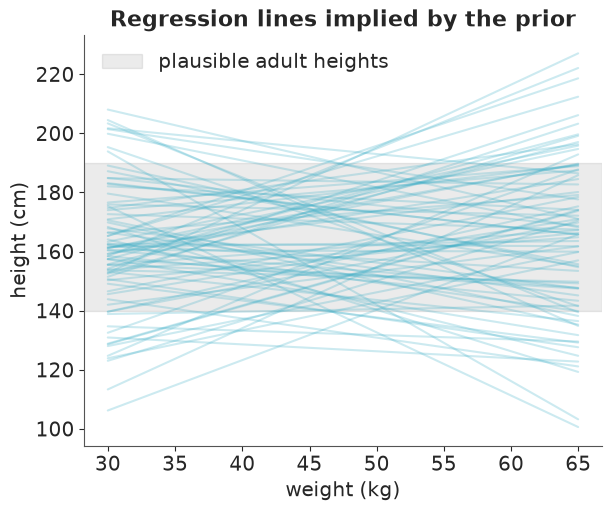
Wide, includes negative slopes we do not really believe in, but nothing crazy. Good enough: the goal of a weakly-informative prior is to rule out the absurd, not to win the argument.

4 · Sample

pm.sample() defaults to 4 chains of 1000 kept draws with NUTS. The warm-up length depends on the sampler: 400 steps under nutpie (the default here), 1000 under PyMC's own NUTS. Pass tune= explicitly when a model needs longer adaptation, and read what actually happened from idata.posterior.attrs["tuning_steps"]. idata.update(...) merges the new groups into the tree we already have.

Another change from older versions: when nutpie (a Rust implementation of NUTS) is installed - and it is in this environment - pm.sample() uses it by default. The log line NUTS[nutpie] tells you so. Pass nuts_sampler="pymc" to get PyMC's own sampler; the two can behave differently on hard geometries, which is worth remembering whenever you compare divergence counts with a tutorial.

with model:
    idata.update(pm.sample(random_seed=RANDOM_SEED))

list(idata.children)

['prior',
 'prior_predictive',
 'observed_data',
 'constant_data',
 'posterior',
 'sample_stats']

5 · Diagnose before you interpret

The order matters. Until the sampler has demonstrably worked, the numbers mean nothing.

r_hat ≤ 1.01: chains agree with one another.
ess_bulk, ess_tail in the hundreds at least: enough effective draws for means and for interval endpoints.
Divergences = 0: NUTS did not hit regions it could not integrate accurately.

# round_to=2 fixes the decimals; the default "auto" keeps 2 significant figures, which is too coarse for alpha
az.summary(idata, ci_kind="hdi", ci_prob=0.94, round_to=2)

	mean	sd	hdi94_lb	hdi94_ub	ess_bulk	ess_tail	r_hat	mcse_mean	mcse_sd
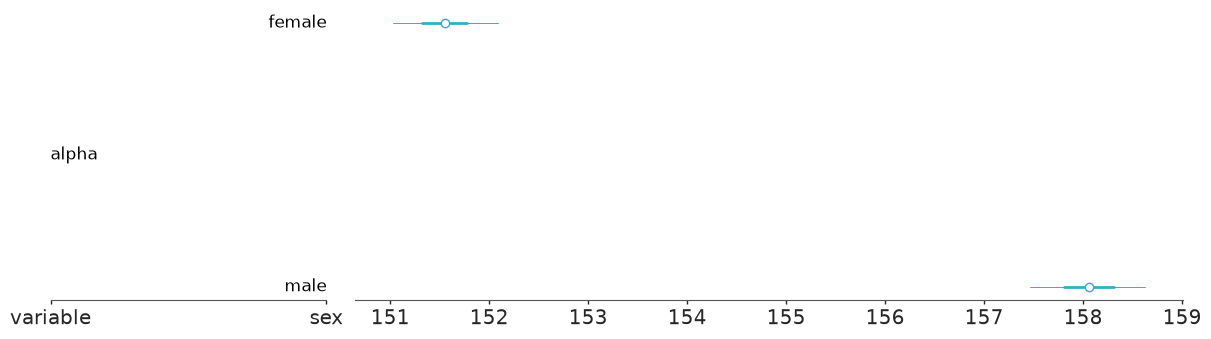
alpha[female]	151.55	0.34	150.94	152.19	3255.56	3255.31	1.0	0.01	0.00
alpha[male]	158.06	0.37	157.37	158.74	3524.44	2969.71	1.0	0.01	0.01
beta	0.64	0.04	0.56	0.72	3097.26	2677.12	1.0	0.00	0.00
sigma	4.29	0.17	3.99	4.62	5203.19	3469.06	1.0	0.00	0.00

print("divergences:", int(idata.sample_stats["diverging"].sum()))
az.plot_trace_dist(idata);

divergences: 0

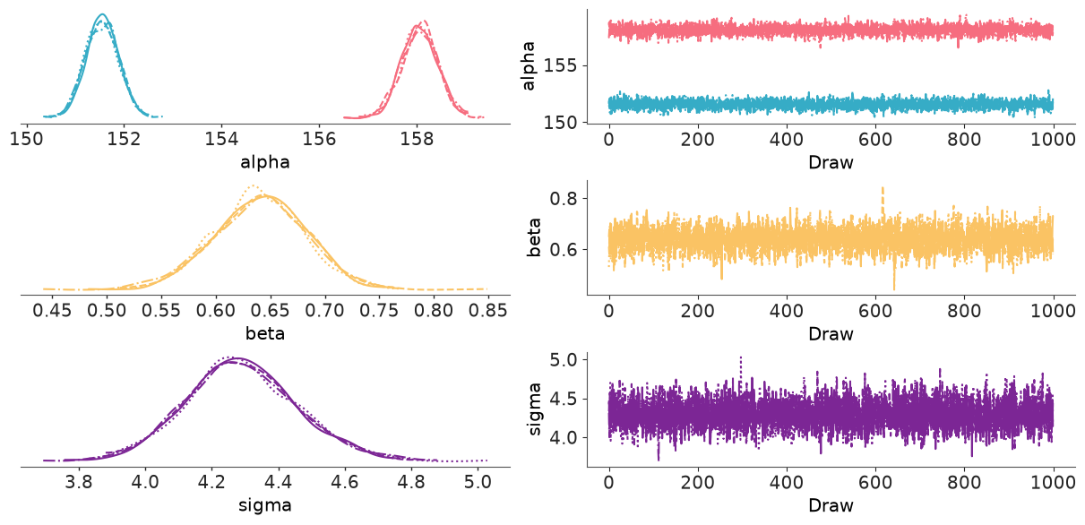
Rank plots are a sharper diagnostic than trace plots: if the chains target the same distribution, each chain's ranks are uniform.

az.plot_rank(idata);

6 · Posterior predictive check: can the model reproduce the data?

with model:
    pm.sample_posterior_predictive(idata, extend_inferencedata=True, random_seed=RANDOM_SEED)

az.plot_ppc_dist(idata);

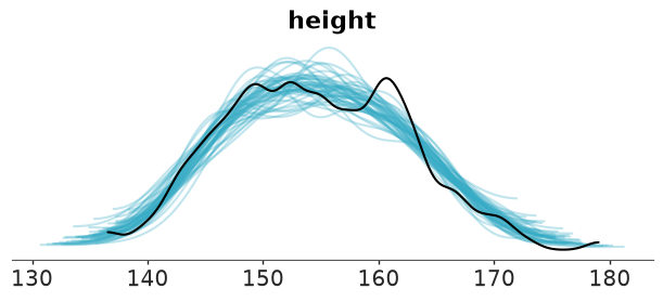
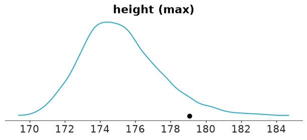
The observed distribution (dark line) sits inside the cloud of replicated datasets. A density overlay is a blunt instrument, so also check a statistic the model was not directly fitted to - here, the tallest person.

az.plot_ppc_tstat(idata, t_stat="max");

7 · Interpret

Work with the posterior as labelled arrays. Because alpha has a sex dimension, the difference between sexes is a one-liner, with full uncertainty.

post = idata.posterior
diff = post["alpha"].sel(sex="male") - post["alpha"].sel(sex="female")

print(f"males are taller at equal weight by {float(diff.mean()):.1f} cm")
print("94% HDI:", az.hdi(diff, prob=0.94).values.round(1))
print(f"P(difference > 5 cm) = {float((diff > 5).mean()):.2f}")

males are taller at equal weight by 6.5 cm
94% HDI: [5.5 7.5]
P(difference > 5 cm) = 1.00

az.plot_forest(idata, var_names=["alpha"], combined=True);

8 · Predict for new inputs

Because inputs were registered with pm.Data, prediction is: swap the data, sample the posterior predictive. predictions=True stores results in a separate predictions group. New coordinates are needed because the obs dimension changes length.

new = pd.DataFrame({"weight": [35.0, 45.0, 55.0, 65.0], "sex": ["female", "female", "male", "male"]})

with model:
    pm.set_data(
        {"weight_c": new.weight - weight_mean, "sex_id": pd.Categorical(new.sex, categories=sexes).codes},
        coords={"obs": new.index},
    )
    pred = pm.sample_posterior_predictive(idata, predictions=True, random_seed=RANDOM_SEED)

pred_height = pred.predictions["height"]
new["mean"] = pred_height.mean(("chain", "draw")).values.round(1)
new[["lo", "hi"]] = az.hdi(pred_height, prob=0.94).values.round(1)
new

	weight	sex	mean	lo	hi
0	35.0	female	145.1	137.1	153.1
1	45.0	female	151.4	143.1	159.2
2	55.0	male	164.4	155.8	172.0
3	65.0	male	170.9	163.0	179.1

Those are predictive intervals for an individual (they include $\sigma$), not intervals for the mean. Know which one your stakeholder is asking for.

9 · Criticise and iterate

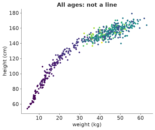
The model is fine for adults. Include the children and a straight line is hopeless:

fig, ax = plt.subplots()
ax.scatter(howell.weight, howell.height, c=howell.age, cmap="viridis", s=12)
ax.set(xlabel="weight (kg)", ylabel="height (cm)", title="All ages: not a line");

Try it yourself

Refit on all ages with log(weight) as the predictor. Is the PPC acceptable?
Let the slope differ by sex (beta with dims="sex"). Does the data support it? Compare with az.compare (you will need pm.compute_log_likelihood).
Replace the Normal likelihood with StudentT. What happens to sigma and to the predictive intervals?

Next: E02 for hierarchical models, or jump into challenge C01.

#1 · Question and data

#2 · Write the model down

#3 · Prior predictive check: what do the priors claim?

#4 · Sample

#5 · Diagnose before you interpret

#6 · Posterior predictive check: can the model reproduce the data?

#7 · Interpret

#8 · Predict for new inputs

#9 · Criticise and iterate

#Try it yourself