Radon is a radioactive gas that seeps into houses from the ground and is the second most common cause of lung cancer. How much of it a house collects depends on the local geology, so levels vary by county - and on where in the house you measure: basements are worse.
The practical question: what radon level should a household in a given county expect? The best-surveyed county has more than a hundred measured homes, so just average them. But a quarter of the counties have three homes or fewer. What do you tell the people who live there?
import arviz as az
import matplotlib.pyplot as plt
import numpy as np
import pandas as pd
import pymc as pm

from pymc_challenges import data

RANDOM_SEED = 1987
rng = np.random.default_rng(RANDOM_SEED)
az.style.use("arviz-variat")
1 · The data
One row per house. log_radon is the log of the measurement in pCi/L, floor is 0 for a
basement measurement and 1 for the first floor, and Uppm is the uranium content of the
county's soil (one value per county - we will need it in section 6).
data.describe("radon")
radon = data.load("radon")
radon[["county", "floor", "log_radon", "Uppm"]].head()
radon: Log radon measurements in 919 Minnesota homes across 85 counties.
  source: US EPA State Residential Radon Survey (Minnesota subset), via Gelman & Hill (2007).
  url:    https://raw.githubusercontent.com/pymc-devs/pymc-examples/main/examples/data/radon.csv
| county | floor | log_radon | Uppm | |
|---|---|---|---|---|
| 0 | AITKIN | 1.0 | 0.832909 | 0.502054 |
| 1 | AITKIN | 0.0 | 0.832909 | 0.502054 |
| 2 | AITKIN | 0.0 | 1.098612 | 0.502054 |
| 3 | AITKIN | 0.0 | 0.095310 | 0.502054 |
| 4 | ANOKA | 0.0 | 1.163151 | 0.428565 |
pd.factorize turns county names into an integer index (county_idx) plus the list of
names (counties). The names become a coordinate; the integers are how each house
looks up its county's parameter. This pair is the backbone of every hierarchical model.
county_idx, counties = pd.factorize(radon.county, sort=True)
n_homes = radon.groupby("county").size().loc[counties]

print(f"{len(radon)} homes, {len(counties)} counties")
print(f"homes per county: median {n_homes.median():.0f}, min {n_homes.min()}, max {n_homes.max()}")
print(f"counties with 3 homes or fewer: {(n_homes <= 3).sum()}")
919 homes, 85 counties
homes per county: median 5, min 1, max 116
counties with 3 homes or fewer: 22
fig, axes = plt.subplots(1, 2, figsize=(11, 3.8))
axes[0].hist(n_homes, bins=np.arange(0, 121, 4))
axes[0].set(xlabel="homes measured in the county", ylabel="number of counties")
for fl, label in [(0, "basement"), (1, "first floor")]:
    axes[1].hist(radon.log_radon[radon.floor == fl], bins=30, alpha=0.6, density=True, label=label)
axes[1].axvline(np.log(4), color="k", ls="--", lw=1)
axes[1].text(np.log(4) + 0.05, 0.62, "EPA action level\n4 pCi/L", fontsize=9)
axes[1].set(xlabel="log radon (log pCi/L)", ylabel="density")
axes[1].legend();
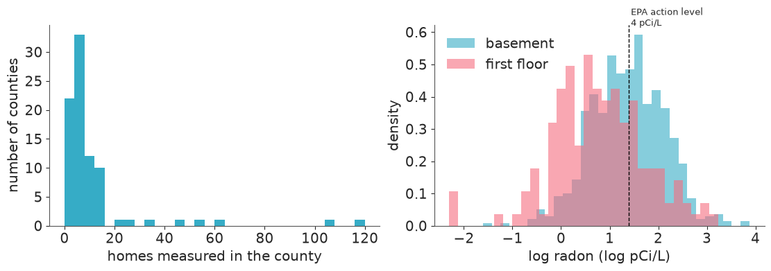
Very unbalanced groups: a couple of counties with around a hundred homes and a long list with a handful. First-floor readings are lower than basement readings, and on the log scale the measurements look roughly Normal.
2 · Two bad answers: complete pooling and no pooling
Throughout, the observation model is
$$\text{log\_radon}_i \sim \text{Normal}(\alpha_{j[i]} + \beta\,\text{floor}_i,\ \sigma)$$
where $j[i]$ is the county of house $i$. The question is what to assume about the county intercepts $\alpha_j$.
- Complete pooling: $\alpha_j = \alpha$ for every county. Counties do not exist.
- No pooling: each $\alpha_j$ gets its own independent, wide prior. Counties have nothing to do with one another.
coords = {"county": counties}
floor = radon.floor.values
log_radon = radon.log_radon.values

with pm.Model() as pooled_model:
    alpha = pm.Normal("alpha", 1, 2)
    beta = pm.Normal("beta", 0, 1)
    sigma = pm.HalfNormal("sigma", 1)
    pm.Normal("y", alpha + beta * floor, sigma, observed=log_radon)
    pooled_idata = pm.sample(random_seed=RANDOM_SEED)

with pm.Model(coords=coords) as unpooled_model:
    alpha = pm.Normal("alpha", 1, 2, dims="county")  # 85 unrelated intercepts
    beta = pm.Normal("beta", 0, 1)
    sigma = pm.HalfNormal("sigma", 1)
    pm.Normal("y", alpha[county_idx] + beta * floor, sigma, observed=log_radon)
    unpooled_idata = pm.sample(random_seed=RANDOM_SEED)

az.summary(pooled_idata, round_to=2)
| mean | sd | eti89_lb | eti89_ub | ess_bulk | ess_tail | r_hat | mcse_mean | mcse_sd | |
|---|---|---|---|---|---|---|---|---|---|
| alpha | 1.36 | 0.03 | 1.32 | 1.41 | 3853.51 | 3232.49 | 1.0 | 0.0 | 0.0 |
| beta | -0.58 | 0.07 | -0.70 | -0.48 | 4062.79 | 3122.23 | 1.0 | 0.0 | 0.0 |
| sigma | 0.79 | 0.02 | 0.76 | 0.82 | 5957.28 | 3274.27 | 1.0 | 0.0 | 0.0 |
alpha[county_idx] is the whole trick: alpha has length 85, county_idx has length 919,
and fancy indexing hands every house the intercept of its own county.
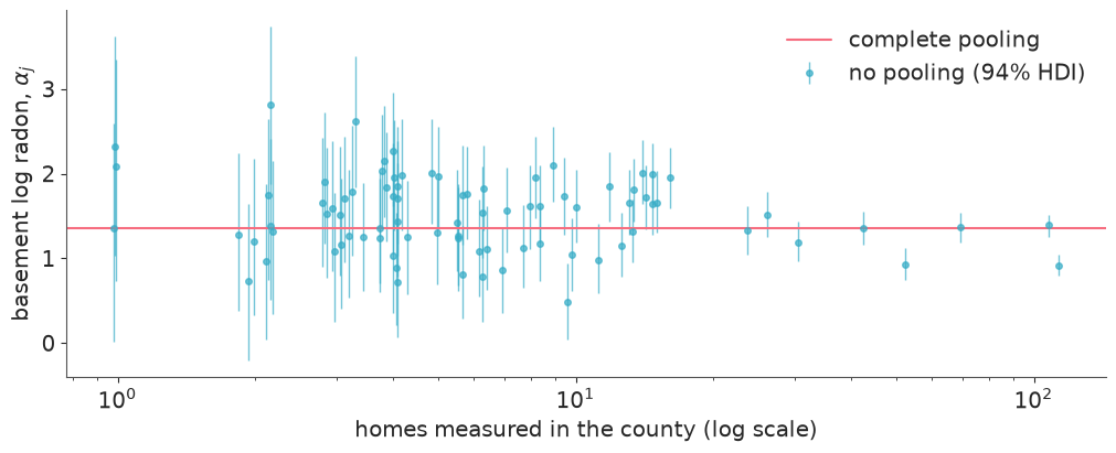
Now the no-pooling estimates, ordered by how many homes back them up:
def county_summary(idata, var="alpha"):
    """Posterior mean and 94% HDI of a county-level variable as a DataFrame indexed by county."""
    post = idata.posterior[var]
    hdi = az.hdi(post, prob=0.94)
    return pd.DataFrame(
        {"mean": post.mean(("chain", "draw")).values, "lo": hdi.sel(ci_bound="lower").values,
         "hi": hdi.sel(ci_bound="upper").values, "n": n_homes.values},
        index=counties,
    )


unpooled = county_summary(unpooled_idata)
pooled_mean = float(pooled_idata.posterior["alpha"].mean())
jitter = np.exp(rng.normal(0, 0.06, len(counties)))  # separate counties with the same n

fig, ax = plt.subplots(figsize=(10, 4))
ax.errorbar(unpooled.n * jitter, unpooled["mean"], yerr=[unpooled["mean"] - unpooled.lo, unpooled.hi - unpooled["mean"]],
            fmt="o", ms=4, lw=1, alpha=0.7, label="no pooling (94% HDI)")
ax.axhline(pooled_mean, color="C1", label="complete pooling")
ax.set(xscale="log", xlabel="homes measured in the county (log scale)", ylabel="basement log radon, $\\alpha_j$")
ax.legend();
unpooled.sort_values("mean").iloc[[0, 1, -2, -1]].round(2)
| mean | lo | hi | n | |
|---|---|---|---|---|
| LAKE | 0.49 | 0.05 | 0.94 | 9 |
| WASECA | 0.71 | 0.07 | 1.40 | 4 |
| WATONWAN | 2.61 | 1.84 | 3.39 | 3 |
| LAC QUI PARLE | 2.81 | 1.88 | 3.73 | 2 |
Both answers are unsatisfying, in opposite ways.
- Complete pooling gives the same number to everyone, although the well-measured counties on the right clearly differ from one another. It underfits.
- No pooling takes every county at face value. The spread of the estimates fans out to the left: every extreme value belongs to a county with fewer than ten homes, and the two highest "county levels" in Minnesota are, on this reading, places where two and three houses were measured. That is what noise looks like. It overfits.
Neither model can say anything about a county with no data at all.
3 · Partial pooling
The hierarchical model adds one assumption: counties are different, but they are all counties in Minnesota - their intercepts come from a common distribution whose mean and spread we learn from the data:
$$ \begin{aligned} \alpha_j &\sim \text{Normal}(\mu_\alpha, \sigma_\alpha) \\ \mu_\alpha &\sim \text{Normal}(1, 2), \qquad \sigma_\alpha \sim \text{HalfNormal}(1) \end{aligned} $$
$\sigma_\alpha$ is the dial between the two extremes above: $\sigma_\alpha \to 0$ is complete pooling, $\sigma_\alpha \to \infty$ is no pooling. We do not set the dial; we put a prior on it and let 85 counties tell us where it sits.
Prior scale: a typical house has 1-10 pCi/L, i.e. log radon between 0 and 2.3. A
HalfNormal(1) on a log-scale standard deviation already allows counties that differ
by a factor of $e^2 \approx 7$. Let us see what the priors imply before fitting.
with pm.Model(coords=coords) as varying_intercept:
    mu_alpha = pm.Normal("mu_alpha", 1, 2)
    sigma_alpha = pm.HalfNormal("sigma_alpha", 1)

    alpha = pm.Normal("alpha", mu_alpha, sigma_alpha, dims="county")
    beta = pm.Normal("beta", 0, 1)
    sigma = pm.HalfNormal("sigma", 1)

    pm.Normal("y", alpha[county_idx] + beta * floor, sigma, observed=log_radon)
    vi_idata = pm.sample_prior_predictive(500, random_seed=RANDOM_SEED)

prior_y = np.exp(vi_idata.prior_predictive["y"].values.ravel())
print("prior predictive radon (pCi/L) quantiles 5% / 50% / 95%:", np.quantile(prior_y, [0.05, 0.5, 0.95]).round(2))
print("observed radon (pCi/L)         quantiles 5% / 50% / 95%:", np.quantile(np.exp(log_radon), [0.05, 0.5, 0.95]).round(2))
prior predictive radon (pCi/L) quantiles 5% / 50% / 95%: [3.0000e-02 2.9900e+00 1.6219e+02]
observed radon (pCi/L)         quantiles 5% / 50% / 95%: [ 1.    3.7  12.21]
The prior predictive distribution has its median in the right place and is about an order of magnitude (or more) wider than the data in both directions. Weakly informative is what we want.
with varying_intercept:
    vi_idata.update(pm.sample(random_seed=RANDOM_SEED))

print("divergences:", int(vi_idata.sample_stats["diverging"].sum()))
az.summary(vi_idata, var_names=["mu_alpha", "sigma_alpha", "beta", "sigma"], ci_kind="hdi", ci_prob=0.94, round_to=2)
divergences: 0
| mean | sd | hdi94_lb | hdi94_ub | ess_bulk | ess_tail | r_hat | mcse_mean | mcse_sd | |
|---|---|---|---|---|---|---|---|---|---|
| mu_alpha | 1.49 | 0.05 | 1.39 | 1.58 | 1560.20 | 1938.20 | 1.0 | 0.0 | 0.0 |
| sigma_alpha | 0.32 | 0.04 | 0.24 | 0.41 | 976.05 | 1327.46 | 1.0 | 0.0 | 0.0 |
| beta | -0.66 | 0.07 | -0.79 | -0.54 | 2657.98 | 2739.92 | 1.0 | 0.0 | 0.0 |
| sigma | 0.73 | 0.02 | 0.69 | 0.76 | 4587.55 | 2659.29 | 1.0 | 0.0 | 0.0 |
Clean diagnostics. The numbers to read are the two standard deviations: homes within a county differ by $\sigma \approx 0.73$, county means differ by only $\sigma_\alpha \approx 0.32$. Most of the variation in radon is between houses, not between counties - so a county average based on two houses is mostly house-to-house noise, and the model knows that.
Shrinkage
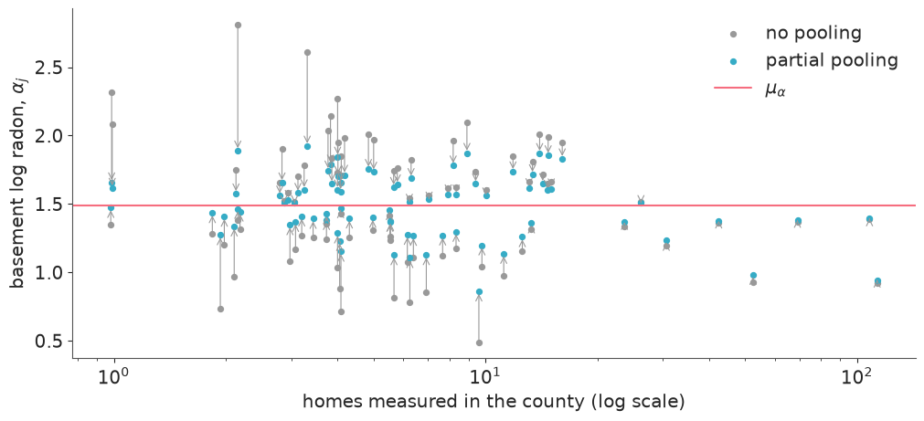
Here are the same counties as before, now with both estimates. Arrows go from the no-pooling estimate to the partial-pooling one.
partial = county_summary(vi_idata)
mu_alpha_mean = float(vi_idata.posterior["mu_alpha"].mean())

fig, ax = plt.subplots(figsize=(10, 4.5))
x = unpooled.n * jitter
ax.scatter(x, unpooled["mean"], s=18, color="0.6", label="no pooling")
ax.scatter(x, partial["mean"], s=18, color="C0", label="partial pooling")
for xi, y0, y1 in zip(x, unpooled["mean"], partial["mean"]):
    ax.annotate("", xy=(xi, y1), xytext=(xi, y0), arrowprops=dict(arrowstyle="->", color="0.6", lw=0.8))
ax.axhline(mu_alpha_mean, color="C1", label="$\\mu_\\alpha$")
ax.set(xscale="log", xlabel="homes measured in the county (log scale)", ylabel="basement log radon, $\\alpha_j$")
ax.legend();
shrink = pd.DataFrame({
    "n": n_homes.values,
    "moved": (partial["mean"] - unpooled["mean"]).abs(),
    "hdi_width_no_pooling": unpooled.hi - unpooled.lo,
    "hdi_width_partial": partial.hi - partial.lo,
})
shrink.groupby(pd.cut(shrink.n, [0, 3, 10, 30, 120])).mean().drop(columns="n").round(2)
| moved | hdi_width_no_pooling | hdi_width_partial | |
|---|---|---|---|
| n | |||
| (0, 3] | 0.27 | 1.79 | 1.01 |
| (3, 10] | 0.18 | 1.15 | 0.84 |
| (10, 30] | 0.08 | 0.73 | 0.63 |
| (30, 120] | 0.02 | 0.35 | 0.34 |
Every estimate moves towards the population mean, and how far depends on how much data the county has. Counties with 1-3 homes move the most and their intervals are almost halved; the large counties on the right hardly move and keep their (already narrow) intervals. Note in passing that $\mu_\alpha$ sits above the complete-pooling line of section 2: the biggest counties happen to have low radon, and complete pooling lets their many houses dominate, whereas $\mu_\alpha$ is the mean over counties. Nobody coded that rule - it is what Bayes' theorem does when a county's own likelihood (weak or strong) meets the population distribution (the prior that the other 84 counties estimated).
For a county with $n_j$ homes the posterior mean is approximately a precision-weighted average
$$\hat\alpha_j \approx \frac{(n_j/\sigma^2)\,\bar y_j + (1/\sigma_\alpha^2)\,\mu_\alpha}{n_j/\sigma^2 + 1/\sigma_\alpha^2}$$
With our estimates, $\sigma^2/\sigma_\alpha^2 \approx 5$: the population prior is worth about five houses. A county with one house keeps roughly 1/6 of its own signal; a county with 100 keeps 95%.
Does shrinkage actually predict better?
It is a fair question - we have biased every estimate on purpose. PSIS-LOO estimates out-of-sample predictive accuracy for each of the three models.
for model, idata in [(pooled_model, pooled_idata), (unpooled_model, unpooled_idata), (varying_intercept, vi_idata)]:
    with model:
        pm.compute_log_likelihood(idata, progressbar=False)

az.compare({"complete pooling": pooled_idata, "no pooling": unpooled_idata, "partial pooling": vi_idata})
| rank | elpd_diff | dse | p_worse | diag_diff | diag_elpd | p | elpd | se | weight | |
|---|---|---|---|---|---|---|---|---|---|---|
| partial pooling | 0 | 0.0 | 0.0 | NaN | 49.4 | -1040.0 | 28.0 | 0.92 | ||
| no pooling | 1 | -20.0 | 6.0 | 1.0 | 4 k̂ > 0.70 | 84.2 | -1060.0 | 29.0 | 0.00 | |
| complete pooling | 2 | -50.0 | 11.0 | 1.0 | 3.7 | -1090.0 | 25.0 | 0.08 |
Partial pooling predicts held-out houses best, by a margin of about three standard errors
over no pooling and more over complete pooling (elpd_diff against dse). Look at column
p, the effective number of parameters: the
no-pooling model spends about 85; the hierarchical model has more parameters on paper
(two hyperparameters on top) but only about 50 effective ones, because shrinkage
restrains them. (No pooling also triggers Pareto-$k$ warnings: in a
county with a single house, leaving that house out changes the county's posterior
completely, which is exactly what importance sampling cannot handle. Its elpd is
therefore approximate - but the ranking is not in doubt.)
4 · When the sampler complains: varying slopes and the funnel
So far NUTS had an easy time. Let us make the model a little more ambitious: maybe the basement/first-floor difference is not the same everywhere (housing stock differs), so give every county its own slope as well:
$$\beta_j \sim \text{Normal}(\mu_\beta, \sigma_\beta)$$
Written exactly like the intercepts - the centred parameterisation.
A note on samplers: in this environment pm.sample() uses nutpie by default. For this
one section we fit with both nutpie and PyMC's own NUTS implementation
(nuts_sampler="pymc"), because they fail in instructively different ways.
with pm.Model(coords=coords) as centred:
    mu_alpha = pm.Normal("mu_alpha", 1, 2)
    sigma_alpha = pm.HalfNormal("sigma_alpha", 1)
    mu_beta = pm.Normal("mu_beta", 0, 1)
    sigma_beta = pm.HalfNormal("sigma_beta", 1)

    alpha = pm.Normal("alpha", mu_alpha, sigma_alpha, dims="county")
    beta = pm.Normal("beta", mu_beta, sigma_beta, dims="county")  # centred: beta_j drawn directly
    sigma = pm.HalfNormal("sigma", 1)

    pm.Normal("y", alpha[county_idx] + beta[county_idx] * floor, sigma, observed=log_radon)

    centred_nutpie = pm.sample(random_seed=RANDOM_SEED)
    centred_idata = pm.sample(nuts_sampler="pymc", random_seed=RANDOM_SEED)
def sampler_report(fits, var="sigma_beta"):
    rows = {}
    for name, idata in fits.items():
        s = az.summary(idata, var_names=[var], round_to=3)
        rows[name] = {
            "divergences": int(idata.sample_stats["diverging"].sum()),
            f"{var} mean": s["mean"].iloc[0], "ess_bulk": s["ess_bulk"].iloc[0], "r_hat": s["r_hat"].iloc[0],
            f"smallest {var} visited": float(idata.posterior[var].min()),
            f"P({var} < 0.05)": float((idata.posterior[var] < 0.05).mean()),
        }
    return pd.DataFrame(rows).T


sampler_report({"centred, nutpie": centred_nutpie, "centred, PyMC NUTS": centred_idata})
| divergences | sigma_beta mean | ess_bulk | r_hat | smallest sigma_beta visited | P(sigma_beta < 0.05) | |
|---|---|---|---|---|---|---|
| centred, nutpie | 7.0 | 0.242 | 36.517 | 1.083 | 0.055712 | 0.0 |
| centred, PyMC NUTS | 104.0 | 0.269 | 34.610 | 1.130 | 0.059106 | 0.0 |
Something is wrong. Both samplers agree on the symptoms that matter: for $\sigma_\beta$,
out of 4000 draws only a few dozen are effectively independent (ess_bulk) and the chains
do not agree with each other (r_hat far above 1.01). PyMC's NUTS also reports about a
hundred divergences; nutpie, which adapts its step size and mass matrix differently,
only a handful. The divergence count is erratic: rerunning this cell with six other seeds
we saw between 41 and 207 with PyMC's NUTS and between 0 and 17 with nutpie - including
nutpie runs with zero divergences whose ESS was still around 60 and whose r_hat was
still 1.05. A low divergence count is not a clean bill of health; always read ESS and
r_hat too.
A divergence means the numerical trajectory flew off the true one because the posterior's
curvature changed faster than the step size could follow. Where they happen tells you
which part of the posterior is the problem. az.plot_pair can mark them:
# a county with no first-floor measurement at all: its slope is informed only by the population
no_first_floor = radon.groupby("county").floor.sum().loc[lambda s: s == 0].index
funnel_county = n_homes.loc[no_first_floor].idxmax()
print(f"{len(no_first_floor)} counties have no first-floor measurement; using {funnel_county} (n = {n_homes[funnel_county]})")

az.plot_pair(
    centred_idata, var_names=["sigma_beta", "beta"], coords={"county": [funnel_county]},
    visuals={"divergence": True}, figure_kwargs={"figsize": (6, 5)},
);
25 counties have no first-floor measurement; using ITASCA (n = 11)
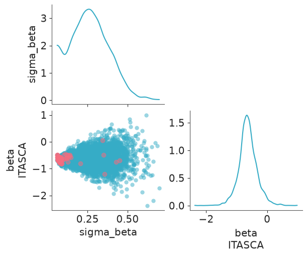
The divergences sit at small $\sigma_\beta$. To see why, put $\sigma_\beta$ on a log scale - this is the space the sampler actually works in.
def funnel_plot(idata, ax, title, y_var="beta"):
    post = az.extract(idata, var_names=["sigma_beta", y_var], keep_dataset=True)
    div = idata.sample_stats["diverging"].stack(sample=("chain", "draw")).values
    yv = post[y_var].sel(county=funnel_county).values
    log_s = np.log(post["sigma_beta"].values)
    ax.scatter(yv[~div], log_s[~div], s=4, alpha=0.3, color="C0")
    ax.scatter(yv[div], log_s[div], s=14, color="crimson", label=f"divergent ({div.sum()})")
    ax.set(title=title, xlabel=f"{y_var}[{funnel_county}]")
    ax.legend(loc="lower right")


fig, ax = plt.subplots(figsize=(5.5, 4.5))
funnel_plot(centred_idata, ax, "centred")
ax.set(ylabel="log $\\sigma_\\beta$");
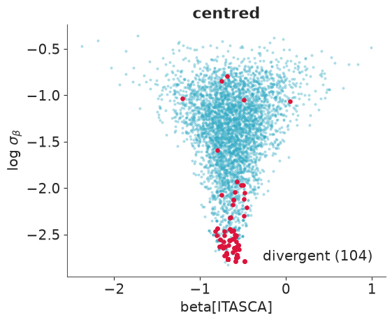
Neal's funnel. When $\sigma_\beta$ is large, $\beta_j$ is free to roam; when $\sigma_\beta$ is small, all 85 $\beta_j$ are squeezed into a tiny interval around $\mu_\beta$. The posterior is wide at the top and needle-thin at the bottom. A step size tuned for the mouth of the funnel overshoots in the neck (divergence), and one tuned for the neck would take forever to cross the mouth. The sampler gives up on the neck: neither run ever visits $\sigma_\beta < 0.05$ (last columns of the table), although nothing in the model or the data rules such values out. Whatever posterior mass lives down there is simply missing from our draws. That is the real damage: not the warning, a potentially wrong answer.
Why did the intercepts not do this? Because $\sigma_\alpha$ is pinned well away from zero by the data (0.32 ± 0.05), so the sampler never needs to visit the neck. The slopes are a different story: only 153 of 919 measurements are on a first floor and 25 counties have none at all, so $\sigma_\beta$ is poorly identified and zero is plausible. Funnels bite when group-level standard deviations are weakly informed - few groups, little data per group, or a true value near zero.
The fix: non-centred parameterisation
Do not tune the sampler (raising target_accept only shrinks the step size and makes the
neck slightly more reachable at a big cost). Change the geometry instead. Sample a
standardised offset and build $\beta_j$ from it:
$$z_j \sim \text{Normal}(0, 1), \qquad \beta_j = \mu_\beta + \sigma_\beta\, z_j$$
The model is identical - same prior on $\beta_j$, same likelihood - but the sampler now moves in $(z_j, \sigma_\beta)$, which are independent a priori. No funnel.
with pm.Model(coords=coords) as noncentred:
    mu_alpha = pm.Normal("mu_alpha", 1, 2)
    sigma_alpha = pm.HalfNormal("sigma_alpha", 1)
    mu_beta = pm.Normal("mu_beta", 0, 1)
    sigma_beta = pm.HalfNormal("sigma_beta", 1)

    z_alpha = pm.Normal("z_alpha", 0, 1, dims="county")
    z_beta = pm.Normal("z_beta", 0, 1, dims="county")
    alpha = pm.Deterministic("alpha", mu_alpha + sigma_alpha * z_alpha, dims="county")
    beta = pm.Deterministic("beta", mu_beta + sigma_beta * z_beta, dims="county")
    sigma = pm.HalfNormal("sigma", 1)

    pm.Normal("y", alpha[county_idx] + beta[county_idx] * floor, sigma, observed=log_radon)
    noncentred_idata = pm.sample(random_seed=RANDOM_SEED)  # default sampler (nutpie)

sampler_report({"centred, nutpie": centred_nutpie, "centred, PyMC NUTS": centred_idata,
                "non-centred, nutpie": noncentred_idata})
| divergences | sigma_beta mean | ess_bulk | r_hat | smallest sigma_beta visited | P(sigma_beta < 0.05) | |
|---|---|---|---|---|---|---|
| centred, nutpie | 7.0 | 0.242 | 36.517 | 1.083 | 0.055712 | 0.000 |
| centred, PyMC NUTS | 104.0 | 0.269 | 34.610 | 1.130 | 0.059106 | 0.000 |
| non-centred, nutpie | 0.0 | 0.262 | 708.992 | 1.005 | 0.000332 | 0.052 |
fig, axes = plt.subplots(1, 3, figsize=(13, 4.2), sharey=True)
funnel_plot(centred_idata, axes[0], "centred")
funnel_plot(noncentred_idata, axes[1], "non-centred: what the sampler sees", y_var="z_beta")
funnel_plot(noncentred_idata, axes[2], "non-centred: implied $\\beta_j$")
axes[0].set(ylabel="log $\\sigma_\\beta$");
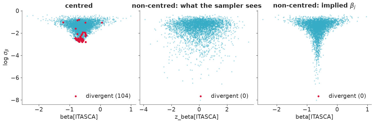
Same model, same data, same seed - only the parameterisation changed. The middle panel
is what NUTS explores now: a shapeless blob, easy. The right panel maps those draws back
to $\beta_j$: the funnel is still there (it is a property of the model), but now its neck
is populated, reaching $\sigma_\beta$ two orders of magnitude smaller than the centred runs
ever visited. The table says how much the centred fits were missing: the region
$\sigma_\beta < 0.05$, to which they gave probability zero, holds about 5% of the
posterior. ESS is up twenty-fold and r_hat is fine.
Be careful what you conclude from the posterior means in that table. The two centred runs disagree with each other (0.24 and 0.27) about as much as with the non-centred one (0.26): with an ESS of 35 their Monte Carlo error swamps the bias from the missing neck. This time the centred answers were not far off. You could not have known that from the centred fits alone - and that is the point of diagnostics.
Rule of thumb. Non-centred is the safe default for hierarchical models. It is not free of trouble, though: it has the mirror-image problem when groups are strongly informed by their own data, because then the likelihood ties $z_j$ and $\sigma$ together instead. Centred is the better choice when every group has lots of data and the group-level sd is clearly non-zero. You can mix: centred for one set of effects, non-centred for another (exercise 2 below looks at this).
And the substantive answer? $\sigma_\beta$ is small and consistent with zero, so there is no strong evidence that the floor effect varies by county:
az.summary(noncentred_idata, var_names=["mu_alpha", "sigma_alpha", "mu_beta", "sigma_beta", "sigma"],
           ci_kind="hdi", ci_prob=0.94, round_to=2)
| mean | sd | hdi94_lb | hdi94_ub | ess_bulk | ess_tail | r_hat | mcse_mean | mcse_sd | |
|---|---|---|---|---|---|---|---|---|---|
| mu_alpha | 1.49 | 0.05 | 1.39 | 1.59 | 1881.43 | 2156.36 | 1.00 | 0.0 | 0.0 |
| sigma_alpha | 0.32 | 0.05 | 0.24 | 0.41 | 1554.36 | 1985.80 | 1.00 | 0.0 | 0.0 |
| mu_beta | -0.65 | 0.08 | -0.79 | -0.49 | 3730.49 | 3056.61 | 1.00 | 0.0 | 0.0 |
| sigma_beta | 0.26 | 0.13 | 0.02 | 0.47 | 708.99 | 988.66 | 1.01 | 0.0 | 0.0 |
| sigma | 0.72 | 0.02 | 0.69 | 0.75 | 4632.53 | 3232.13 | 1.00 | 0.0 | 0.0 |
5 · Aside: pm.ZeroSumNormal
There is a second, subtler geometry problem in every varying-intercept model: you can add a constant to $\mu_\alpha$ and subtract it from all the offsets and the likelihood does not change - only the prior holds them in place. With many groups that is harmless; with few groups, or several crossed factors (team attack + team defence + home advantage...), it becomes a real identifiability problem.
pm.ZeroSumNormal is the modern tool: a Normal whose values are constrained to sum to
zero along a dimension. The intercept is then unambiguously "the average county", and
the offsets are deviations from it.
with pm.Model(coords=coords) as zerosum_model:
    mu_alpha = pm.Normal("mu_alpha", 1, 2)
    sigma_alpha = pm.HalfNormal("sigma_alpha", 1)
    offset = pm.ZeroSumNormal("offset", sigma=sigma_alpha, dims="county")
    alpha = pm.Deterministic("alpha", mu_alpha + offset, dims="county")
    beta = pm.Normal("beta", 0, 1)
    sigma = pm.HalfNormal("sigma", 1)
    pm.Normal("y", alpha[county_idx] + beta * floor, sigma, observed=log_radon)
    zerosum_idata = pm.sample(random_seed=RANDOM_SEED)

pd.concat({
    "Normal(mu, sigma)": az.summary(vi_idata, var_names=["mu_alpha", "sigma_alpha"], round_to=3),
    "mu + ZeroSumNormal": az.summary(zerosum_idata, var_names=["mu_alpha", "sigma_alpha"], round_to=3),
})[["mean", "sd", "ess_bulk", "r_hat"]]
| mean | sd | ess_bulk | r_hat | ||
|---|---|---|---|---|---|
| Normal(mu, sigma) | mu_alpha | 1.490 | 0.050 | 1560.201 | 1.002 |
| sigma_alpha | 0.319 | 0.045 | 976.046 | 1.001 | |
| mu + ZeroSumNormal | mu_alpha | 1.492 | 0.036 | 1739.040 | 1.001 |
| sigma_alpha | 0.319 | 0.046 | 721.731 | 1.005 |
zs = county_summary(zerosum_idata)
print("largest difference in county intercepts between the two models:",
      float((zs["mean"] - partial["mean"]).abs().max().round(3)))
largest difference in county intercepts between the two models: 0.01
The county estimates are the same to within Monte Carlo error, $\sigma_\alpha$ is the same,
but $\mu_\alpha$ has a smaller posterior sd. That is not a free lunch, it is a different
question: with ZeroSumNormal, $\mu_\alpha$ is the mean of these 85 counties; in the
standard model it is the mean of the population counties are drawn from, which is less
certain. Use the standard form when you want to generalise to new groups (section 7);
use ZeroSumNormal when the groups are the whole population of interest and you want
identifiable, well-behaved offsets. Challenge C02 needs it.
6 · A group-level predictor: uranium
Shrinking towards the state average is sensible when you know nothing else about a county. But we do: radon comes from uranium in the soil, and we have a soil measurement per county. Let the population mean itself depend on it:
$$\alpha_j \sim \text{Normal}(\gamma_0 + \gamma_1\, \log u_j,\ \sigma_\alpha)$$
Small counties are now shrunk towards the regression line - towards counties with
similar geology - rather than towards one grand mean. We go back to a common floor effect
(section 4 found no evidence for varying slopes), use the non-centred form, and register
inputs with pm.Data. Note the two different dims: log_u lives on county, the
observations on obs.
log_u = np.log(radon.groupby("county").Uppm.first().loc[counties].values)
coords = {"county": counties, "obs": radon.index}

with pm.Model(coords=coords) as uranium_model:
    county_id = pm.Data("county_id", county_idx, dims="obs")
    floor_d = pm.Data("floor", floor, dims="obs")
    log_u_d = pm.Data("log_u", log_u, dims="county")

    gamma_0 = pm.Normal("gamma_0", 1, 2)
    gamma_1 = pm.Normal("gamma_1", 0, 1)
    sigma_alpha = pm.HalfNormal("sigma_alpha", 1)
    z = pm.Normal("z", 0, 1, dims="county")
    alpha = pm.Deterministic("alpha", gamma_0 + gamma_1 * log_u_d + sigma_alpha * z, dims="county")

    beta = pm.Normal("beta", 0, 1)
    sigma = pm.HalfNormal("sigma", 1)

    pm.Normal("y", alpha[county_id] + beta * floor_d, sigma, observed=log_radon, dims="obs")
    uranium_idata = pm.sample(random_seed=RANDOM_SEED)

print("divergences:", int(uranium_idata.sample_stats["diverging"].sum()))
az.summary(uranium_idata, var_names=["gamma_0", "gamma_1", "sigma_alpha", "beta", "sigma"],
           ci_kind="hdi", ci_prob=0.94, round_to=2)
divergences: 0
| mean | sd | hdi94_lb | hdi94_ub | ess_bulk | ess_tail | r_hat | mcse_mean | mcse_sd | |
|---|---|---|---|---|---|---|---|---|---|
| gamma_0 | 1.49 | 0.04 | 1.43 | 1.57 | 1620.41 | 1924.47 | 1.0 | 0.0 | 0.0 |
| gamma_1 | 0.69 | 0.09 | 0.53 | 0.86 | 2039.49 | 2391.06 | 1.0 | 0.0 | 0.0 |
| sigma_alpha | 0.15 | 0.05 | 0.06 | 0.24 | 733.67 | 953.59 | 1.0 | 0.0 | 0.0 |
| beta | -0.63 | 0.07 | -0.76 | -0.51 | 3002.27 | 2332.17 | 1.0 | 0.0 | 0.0 |
| sigma | 0.73 | 0.02 | 0.70 | 0.76 | 3376.27 | 2779.08 | 1.0 | 0.0 | 0.0 |
post = az.extract(uranium_idata, var_names=["gamma_0", "gamma_1"])
u_grid = np.linspace(log_u.min() - 0.05, log_u.max() + 0.05, 50)
lines = post["gamma_0"].values[:, None] + post["gamma_1"].values[:, None] * u_grid
with_u = county_summary(uranium_idata)

fig, ax = plt.subplots(figsize=(8, 4.5))
ax.fill_between(u_grid, *np.quantile(lines, [0.03, 0.97], axis=0), color="C1", alpha=0.3)
ax.plot(u_grid, lines.mean(axis=0), color="C1", label="$\\gamma_0 + \\gamma_1 \\log u$")
ax.errorbar(log_u, with_u["mean"], yerr=[with_u["mean"] - with_u.lo, with_u.hi - with_u["mean"]],
            fmt="o", ms=3, lw=0.7, alpha=0.7, label="county intercepts $\\alpha_j$ (94% HDI)")
ax.set(xlabel="log uranium (ppm)", ylabel="basement log radon")
ax.legend();
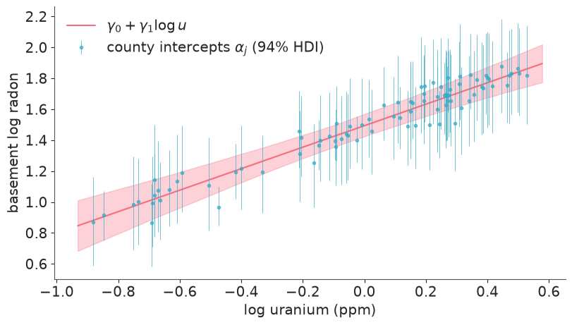
Uranium explains a large part of the between-county differences: $\gamma_1$ is clearly positive, and $\sigma_\alpha$ - the county variation left unexplained - has roughly halved compared with section 3. The remaining county effects hug the line. A good group-level predictor makes partial pooling stronger, because the thing being pooled towards is better.
Posterior predictive check
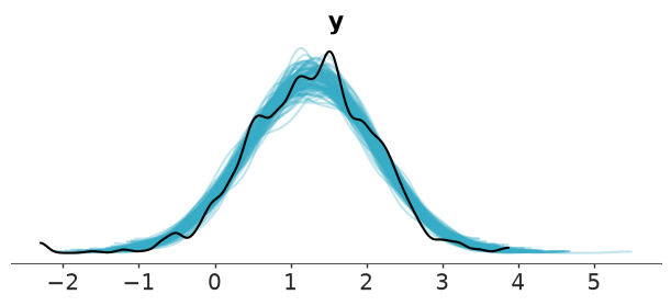
Does the model reproduce the data? First the overall distribution, then a statistic that matters for the application and that the model never saw directly: the share of homes above the EPA action level of 4 pCi/L.
with uranium_model:
    pm.sample_posterior_predictive(uranium_idata, extend_inferencedata=True, random_seed=RANDOM_SEED)

az.plot_ppc_dist(uranium_idata, num_samples=100);
y_rep = az.extract(uranium_idata, group="posterior_predictive", var_names="y").values  # (obs, sample)
share_rep = (y_rep > np.log(4)).mean(axis=0)
share_obs = (log_radon > np.log(4)).mean()

fig, ax = plt.subplots(figsize=(6, 3.5))
ax.hist(share_rep, bins=30, alpha=0.7)
ax.axvline(share_obs, color="k", label=f"observed = {share_obs:.2f}")
ax.set(xlabel="share of homes above 4 pCi/L", ylabel="replicated datasets")
ax.legend();
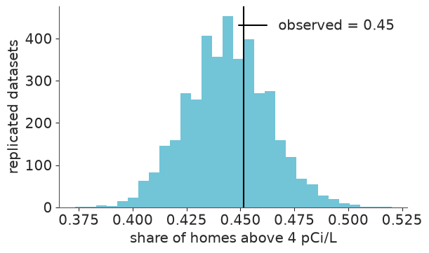
The replicated datasets look like the real one (the small bump at the far left of the observed curve is three readings at 0.1 pCi/L, the lowest value recorded), and the observed share of homes above the action level is a typical value under the model.
7 · Predicting for a county we have never seen
This is where hierarchical models earn their keep. Suppose a new county is surveyed for soil uranium (say 1.2 ppm) but not a single house has been measured. No pooling has nothing to say. The hierarchical model says: its intercept is one more draw from the population distribution.
The cleanest way to do this in PyMC is to extend the fitted model with new random
variables that reuse the posterior of the hyperparameters, then ask
sample_posterior_predictive for just those variables. They were not in the posterior, so
PyMC forward-samples them, once per posterior draw.
NEW_U = 1.2  # ppm

with uranium_model:
    alpha_new = pm.Normal("alpha_new", gamma_0 + gamma_1 * np.log(NEW_U), sigma_alpha)
    # a new house in the new county: basement, first floor
    pm.Normal("y_new", alpha_new + beta * np.array([0.0, 1.0]), sigma, shape=2)
    new_pred = pm.sample_posterior_predictive(
        uranium_idata, var_names=["alpha_new", "y_new"], predictions=True, random_seed=RANDOM_SEED
    )

y_new = new_pred.predictions["y_new"]
for i, where in enumerate(["basement", "first floor"]):
    draws = np.exp(y_new.isel(y_new_dim_0=i).values.ravel())
    lo, hi = np.quantile(draws, [0.03, 0.97])
    print(f"new county, {where:<11}: median {np.median(draws):.1f} pCi/L, 94% interval [{lo:.1f}, {hi:.1f}], "
          f"P(> 4 pCi/L) = {(draws > 4).mean():.2f}")
new county, basement   : median 5.1 pCi/L, 94% interval [1.2, 20.1], P(> 4 pCi/L) = 0.63
new county, first floor: median 2.7 pCi/L, 94% interval [0.6, 11.2], P(> 4 pCi/L) = 0.30
How much do we lose by not having measured anything there? Compare the new county's intercept with the known counties whose uranium level is most similar:
alpha_new_draws = new_pred.predictions["alpha_new"]
closest = pd.Series(np.abs(log_u - np.log(NEW_U)), index=counties).nsmallest(3).index
rows = {"NEW COUNTY (no homes)": {"n": 0, "mean": float(alpha_new_draws.mean()), "sd": float(alpha_new_draws.std())}}
for c in closest:
    a = uranium_idata.posterior["alpha"].sel(county=c)
    rows[c] = {"n": int(n_homes[c]), "mean": float(a.mean()), "sd": float(a.std())}
pd.DataFrame(rows).T.round(2)
| n | mean | sd | |
|---|---|---|---|
| NEW COUNTY (no homes) | 0.0 | 1.62 | 0.16 |
| WATONWAN | 3.0 | 1.74 | 0.17 |
| RICE | 11.0 | 1.70 | 0.13 |
| LE SUEUR | 5.0 | 1.65 | 0.14 |
The new county's intercept is centred on the regression line, with an sd that combines the unexplained county variation $\sigma_\alpha$ with the uncertainty in the line itself. Remarkably, that is barely wider than for comparable counties where a handful of homes were measured: once uranium is known, a few noisy houses ($\sigma \approx 0.73$ each) add little about the county. And for predicting a single house, house-to-house variation dominates everything else - which is why the predictive intervals above span more than a factor of ten. The honest advice to a homeowner anywhere in Minnesota: the county tells you the odds, but test your own basement.
Try it yourself
- Correlated effects. In section 4 intercepts and slopes were independent. Give each
county a bivariate Normal $(\alpha_j, \beta_j)$ with
pm.LKJCholeskyCov(non-centred:mu + chol @ z). Is there evidence that high-radon counties have a different floor effect? - No parameterisation is perfect. Refit the non-centred model of section 4 with
nuts_sampler="pymc". With this seed we got about 20 divergences even there. Usefunnel_plotto see where they live - the neck again, or somewhere else? Then try a mixed model (centredalpha, non-centredbeta) andtarget_accept=0.95. - A contextual effect. Counties where many homes are measured on the first floor
(few basements) may differ systematically. Add the county mean of
flooras a second group-level predictor next to uranium. What happens tobetaand $\sigma_\alpha$?
Next: E03, or put this to work in challenge C02 (Premier League), where the groups are football teams and the identifiability problem of section 5 is centre stage.