A generalised linear model is a linear regression wearing two adapters: a link function that maps the linear predictor onto the scale of the mean, and a likelihood that matches the kind of data you have. For a yes/no outcome:
$$ y_i \sim \text{Bernoulli}(p_i), \qquad \text{logit}(p_i) = \log\frac{p_i}{1-p_i} = \alpha + x_i^\top \beta $$
Writing that down in PyMC takes four lines. Everything that is hard about it - and everything this notebook is about - comes from the link: coefficients live on the log-odds scale, where neither priors nor posteriors mean what your intuition says they mean.
import arviz as az
import matplotlib.pyplot as plt
import numpy as np
import pandas as pd
import pymc as pm
from scipy.special import expit

from pymc_challenges import data

RANDOM_SEED = 2007
rng = np.random.default_rng(RANDOM_SEED)
az.style.use("arviz-variat")
1 · Question and data
Many wells in Bangladesh are contaminated with natural arsenic. A research team measured the wells in one area, told every household its level, and encouraged those above the safety limit (0.5 in the units used here, hundreds of micrograms per litre) to switch to a safe well nearby. A few years later they came back and recorded who had switched.
What drives the decision to switch - and by how much, in units a public-health planner can use? The data are from Gelman & Hill (2007), who use them for exactly this lesson.
data.describe("wells")
raw = data.load("wells")
raw.head()
wells: Whether 3020 households switched wells after learning theirs was unsafe.
  source: Bangladesh arsenic survey, Gelman & Hill (2007), via R package `carData`.
  url:    https://vincentarelbundock.github.io/Rdatasets/csv/carData/Wells.csv
| switch | arsenic | distance | education | association | |
|---|---|---|---|---|---|
| rownames | |||||
| 1 | yes | 2.36 | 16.826 | 0 | no |
| 2 | yes | 0.71 | 47.322 | 0 | no |
| 3 | no | 2.07 | 20.967 | 10 | no |
| 4 | yes | 1.15 | 21.486 | 12 | no |
| 5 | yes | 1.10 | 40.874 | 14 | yes |
Only households with an unsafe well are in the data, which is why arsenic starts at
0.51. distance is the distance in metres to the nearest known safe well, education the
years of schooling of the head of household, association whether anyone in the household
takes part in community organisations.
def prepare(df):
    """Add the modelling columns. Used again later on counterfactual copies of the data."""
    return df.assign(
        y=(df["switch"] == "yes").astype(int),
        dist100=df["distance"] / 100,  # units of 100 m
        log_arsenic=np.log(df["arsenic"]),
        educ4=df["education"] / 4,  # units of 4 years of schooling
        assoc=(df["association"] == "yes").astype(int),
    )


wells = prepare(raw)
print(f"{wells.y.mean():.1%} of {len(wells)} households switched")
wells[["distance", "arsenic", "education"]].describe().round(2)
57.5% of 3020 households switched
| distance | arsenic | education | |
|---|---|---|---|
| count | 3020.00 | 3020.00 | 3020.00 |
| mean | 48.33 | 1.66 | 4.83 |
| std | 38.48 | 1.11 | 4.02 |
| min | 0.39 | 0.51 | 0.00 |
| 25% | 21.12 | 0.82 | 0.00 |
| 50% | 36.76 | 1.30 | 5.00 |
| 75% | 64.04 | 2.20 | 8.00 |
| max | 339.53 | 9.65 | 17.00 |
def binned_rate(x, y, n_bins=12):
    """Mean of y within quantile bins of x, with a +/- 2 standard error bar."""
    bins = pd.qcut(x, n_bins, duplicates="drop")
    g = pd.DataFrame({"x": x, "y": y}).groupby(bins, observed=True)
    out = g.agg(x=("x", "mean"), rate=("y", "mean"), n=("y", "size"))
    out["se"] = np.sqrt(out.rate * (1 - out.rate) / out.n)
    return out


fig, axes = plt.subplots(1, 2, figsize=(11, 3.8), sharey=True)
for ax, col, label in zip(axes, ["distance", "arsenic"], ["distance to nearest safe well (m)", "arsenic level"]):
    b = binned_rate(wells[col], wells.y)
    ax.errorbar(b.x, b.rate, yerr=2 * b.se, fmt="o", color="k", ms=4)
    ax.set(xlabel=label, ylim=(0, 1))
axes[0].set_ylabel("share that switched");
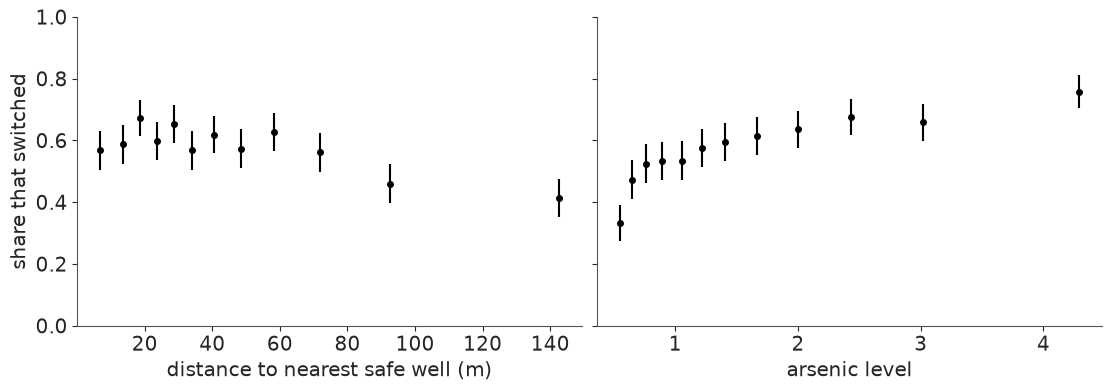
A scatter plot of a 0/1 outcome is two stripes of dots, so we plot the switching rate in bins instead. Further to walk: less switching. More arsenic: more switching, but the curve flattens - remember that for later.
2 · Scale the predictors before you think about priors
A prior is a statement about a coefficient, and a coefficient is "change in log-odds per unit of x". In metres, the distance coefficient would be around -0.006: what prior is "weakly informative" for that? Nobody knows without doing arithmetic. So change the units until a coefficient of 1 is a big but conceivable effect:
dist100: distance in units of 100 m (most households are within 100 m of a safe well).educ4: education in units of 4 years.- arsenic is already of order 1.
We also centre every predictor. Then $\alpha$ is the log-odds of switching for an average household - something we can reason about - instead of for a household with zero arsenic living on top of a safe well, which does not exist. Centring also makes main effects readable when we add interactions.
A model in this notebook is a list of terms; "a:b" means the product of two centred columns.
CENTRE = wells[["dist100", "arsenic", "log_arsenic", "educ4", "assoc"]].mean()


def design(df, terms):
    """Centred design matrix for a list of terms such as ["dist100", "arsenic", "dist100:arsenic"]."""
    Z = df[CENTRE.index] - CENTRE  # centred with the means of the OBSERVED data, always
    return pd.DataFrame({t: Z[t.split(":")].prod(axis=1) for t in terms}, index=df.index)


design(wells, ["dist100", "arsenic", "dist100:arsenic"]).head(3).round(3)
| dist100 | arsenic | dist100:arsenic | |
|---|---|---|---|
| rownames | |||
| 1 | -0.315 | 0.703 | -0.222 |
| 2 | -0.010 | -0.947 | 0.010 |
| 3 | -0.274 | 0.413 | -0.113 |
3 · The model, and what priors look like through a logit link
One function builds every model we fit today. The two prior scales are arguments because we are about to compare two choices.
def logistic_model(X, y, sigma_alpha=1.5, sigma_beta=1.0):
    coords = {"predictor": list(X.columns), "obs": X.index}
    with pm.Model(coords=coords) as model:
        alpha = pm.Normal("alpha", 0, sigma_alpha)
        beta = pm.Normal("beta", 0, sigma_beta, dims="predictor")
        eta = alpha + pm.math.dot(X.values, beta)  # the linear predictor, on the log-odds scale
        pm.Bernoulli("switch", logit_p=eta, observed=y, dims="obs")  # logit_p applies the inverse link
    return model


X1 = design(wells, ["dist100"])
logistic_model(X1, wells.y)
"When in doubt, make the prior wide" is a fine instinct on the scale of the outcome. On
the logit scale it backfires. Let us simulate from a "vague" Normal(0, 10) on both
parameters and from the defaults above, and look at what each claims about probabilities.
d_grid = np.linspace(0, 3.4, 100)  # distance grid in units of 100 m
priors = {"'vague': sd 10 on both": (10, 10), "weakly informative: sd 1.5 and 1": (1.5, 1.0)}

fig, axes = plt.subplots(2, 2, figsize=(11, 6.5))
for row, (label, (s_a, s_b)) in zip(axes, priors.items()):
    with logistic_model(X1, wells.y, s_a, s_b):
        prior_idata = pm.sample_prior_predictive(1000, random_seed=RANDOM_SEED)
    pr = az.extract(prior_idata, group="prior")
    a, b = pr["alpha"].values, pr["beta"].sel(predictor="dist100").values

    curves = expit(a[:, None] + b[:, None] * (d_grid - CENTRE["dist100"]))
    row[0].plot(d_grid * 100, curves[:60].T, color="C0", alpha=0.35)
    row[0].set(xlabel="distance (m)", ylabel="P(switch)", title=label, ylim=(-0.02, 1.02))

    # implied probability of switching for every household, pooled over prior draws
    p_households = expit(a[:, None] + b[:, None] * X1["dist100"].values)
    row[1].hist(p_households.ravel(), bins=40, density=True, color="C0")
    row[1].set(xlabel="P(switch) for a household", yticks=[], title="implied prior on P(switch)");
    print(f"{label}: {np.mean((p_households < 0.01) | (p_households > 0.99)):.0%} of prior mass on P < 1% or P > 99%")
'vague': sd 10 on both: 67% of prior mass on P < 1% or P > 99%
weakly informative: sd 1.5 and 1: 0% of prior mass on P < 1% or P > 99%
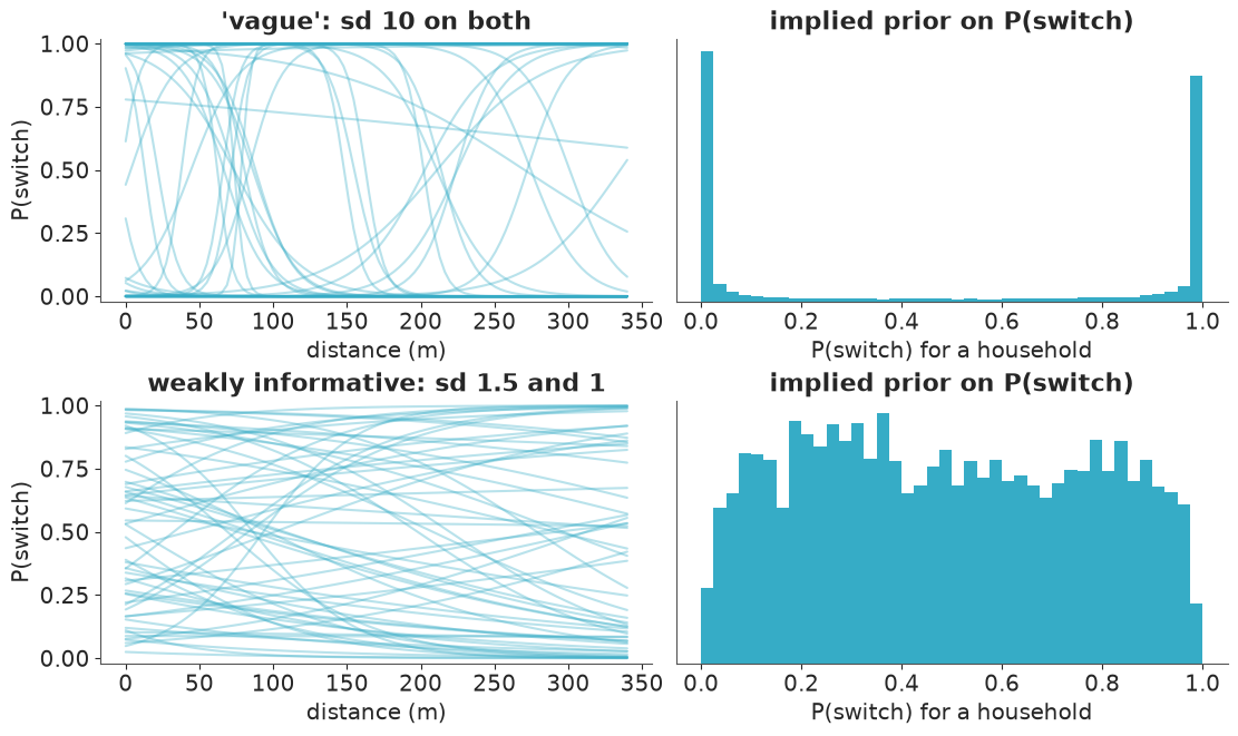
The "vague" prior is anything but. A log-odds of ±10 is a probability of 0.00005 or
0.99995, so Normal(0, 10) says: almost every household either certainly switches or
certainly does not, and moving a few metres flips the village from one to the other. That is
a strong, bizarre belief - the prior on the probability scale is a bathtub, with two thirds
of its mass below 1% or above 99%.
The weakly-informative version spreads over the whole probability scale, allows steep curves in both directions, and only rules out cliffs. With 3020 observations either prior will be overwhelmed for the main effects. With few observations, rare outcomes, or perfectly separating predictors it will not, and the bathtub prior actively hurts. Always check GLM priors on the outcome scale.
4 · Fit, diagnose, interpret: distance only
The helper below samples, optionally adds posterior predictive draws (for the calibration checks in section 7), and computes PSIS-LOO, which section 8 explains. LOO needs the pointwise log-likelihood, a 4000 x 3020 array of about 100 MB per model. We fit five models, and a notebook kernel never frees anything you still hold a name for, so the helper keeps the small LOO result and deletes the big array straight away. On a laptop this is the difference between a notebook that peaks above 3 GB and one that stays well under 2.
def fit(terms, ppc=False):
    """Fit a logistic model with these terms; return (DataTree, PSIS-LOO result)."""
    with logistic_model(design(wells, terms), wells.y):
        idata = pm.sample(random_seed=RANDOM_SEED)
        if ppc:
            pm.sample_posterior_predictive(idata, extend_inferencedata=True, random_seed=RANDOM_SEED)
        pm.compute_log_likelihood(idata, progressbar=False)  # pointwise log-likelihood, needed for LOO
    loo = az.loo(idata, pointwise=True)  # see section 8
    # Two ~100 MB arrays we no longer need: the log-likelihood that LOO has consumed, and the
    # importance weights that ArviZ keeps on the result (compare and plot_khat do not use them).
    del idata["log_likelihood"]
    loo.log_weights = None
    print("divergences:", int(idata.sample_stats["diverging"].sum()))
    return idata, loo


idatas, loos = {}, {}
idatas["dist"], loos["dist"] = fit(["dist100"])
az.summary(idatas["dist"], var_names=["alpha", "beta"], ci_kind="hdi", ci_prob=0.94, round_to=2)
divergences: 0
| mean | sd | hdi94_lb | hdi94_ub | ess_bulk | ess_tail | r_hat | mcse_mean | mcse_sd | |
|---|---|---|---|---|---|---|---|---|---|
| alpha | 0.30 | 0.04 | 0.24 | 0.38 | 4282.75 | 2677.55 | 1.0 | 0.0 | 0.0 |
| beta[dist100] | -0.62 | 0.09 | -0.79 | -0.43 | 3998.01 | 2990.62 | 1.0 | 0.0 | 0.0 |
Diagnostics are clean (r_hat of 1.00, ESS in the thousands, no divergences), so we may
interpret.
The intercept. Predictors are centred, so expit(alpha) is the switching probability
for a household at the average distance of 48 m.
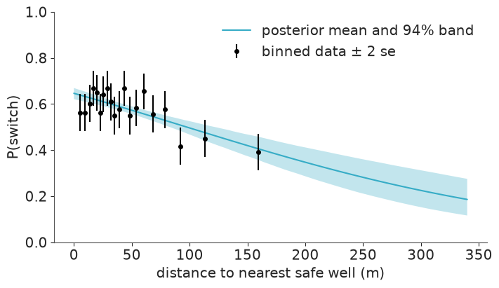
The slope, and the divide-by-4 rule. The logistic curve is steepest at $p = 0.5$, where its slope is $\beta/4$. So $\beta / 4$ is an upper bound on the change in probability per unit of $x$ - and a good approximation whenever probabilities are between roughly 0.25 and 0.75, as they are here.
post = idatas["dist"].posterior
beta_dist = post["beta"].sel(predictor="dist100")
print(f"P(switch) at average distance: {float(expit(post['alpha']).mean()):.2f}")
print(f"divide-by-4: 100 m further away lowers P(switch) by at most {-25 * float(beta_dist.mean()):.1f} percentage points")
P(switch) at average distance: 0.58
divide-by-4: 100 m further away lowers P(switch) by at most 15.5 percentage points
def predict_p(idata, X, num_samples=1000):
    """Posterior draws of P(switch) for the rows of a design matrix: array (draws, rows)."""
    draws = az.extract(idata, var_names=["alpha", "beta"], num_samples=num_samples, random_seed=RANDOM_SEED)
    beta = draws["beta"].transpose("sample", "predictor").values
    return expit(draws["alpha"].values[:, None] + beta @ X.values.T)


grid = prepare(pd.DataFrame({"distance": d_grid * 100, "arsenic": 1.0, "education": 0, "switch": "no", "association": "no"}))
p_grid = predict_p(idatas["dist"], design(grid, ["dist100"]))

b = binned_rate(wells.distance, wells.y, n_bins=20)
fig, ax = plt.subplots(figsize=(7, 4))
ax.fill_between(grid.distance, *np.quantile(p_grid, [0.03, 0.97], axis=0), alpha=0.3)
ax.plot(grid.distance, p_grid.mean(axis=0), label="posterior mean and 94% band")
ax.errorbar(b.x, b.rate, yerr=2 * b.se, fmt="o", color="k", ms=4, label="binned data ± 2 se")
ax.set(xlabel="distance to nearest safe well (m)", ylabel="P(switch)", ylim=(0, 1))
ax.legend();
5 · Add arsenic, then ask a better question than "what is beta?"
idatas["dist + arsenic"], loos["dist + arsenic"] = fit(["dist100", "arsenic"], ppc=True)
az.summary(idatas["dist + arsenic"], var_names=["alpha", "beta"], ci_kind="hdi", ci_prob=0.94, round_to=2)
divergences: 0
| mean | sd | hdi94_lb | hdi94_ub | ess_bulk | ess_tail | r_hat | mcse_mean | mcse_sd | |
|---|---|---|---|---|---|---|---|---|---|
| alpha | 0.33 | 0.04 | 0.26 | 0.41 | 5354.40 | 2955.81 | 1.0 | 0.0 | 0.0 |
| beta[dist100] | -0.89 | 0.10 | -1.09 | -0.70 | 5671.24 | 3342.28 | 1.0 | 0.0 | 0.0 |
| beta[arsenic] | 0.46 | 0.04 | 0.38 | 0.54 | 5050.81 | 3095.49 | 1.0 | 0.0 | 0.0 |
Both effects have the expected sign, and the distance coefficient became more negative once arsenic entered (-0.62 before, -0.89 now). That happens when predictors are correlated in the "masking" direction: households far from a safe well tend to have somewhat higher arsenic (correlation 0.18, printed below), so in the distance-only model the two effects partly cancelled.
Which predictor matters more? Coefficients cannot say: they are per unit, and "1 unit of arsenic" and "100 m" are not comparable. They are also on the wrong scale. The planner's question is about probabilities, and because of the non-linear link the effect of distance on probability is different for every household.
The honest summary is an average predictive difference: take every household as it is, set the predictor to a low value, then to a high value, leave everything else alone, and average the change in predicted probability over households. Do it once per posterior draw and you get a posterior distribution for the answer.
print(f"correlation of distance and arsenic: {wells.distance.corr(wells.arsenic):.2f}")


def average_predictive_difference(idata, terms, column, lo, hi):
    """Posterior draws of mean_i[ P(switch | column=hi, rest_i) - P(switch | column=lo, rest_i) ]."""
    p_lo = predict_p(idata, design(prepare(raw.assign(**{column: lo})), terms))
    p_hi = predict_p(idata, design(prepare(raw.assign(**{column: hi})), terms))
    return (p_hi - p_lo).mean(axis=1)


def report(apd, label):
    lo, hi = np.quantile(apd, [0.03, 0.97])
    print(f"{label:<42} {apd.mean():+.3f}   94% interval [{lo:+.3f}, {hi:+.3f}]")


terms = ["dist100", "arsenic"]
report(average_predictive_difference(idatas["dist + arsenic"], terms, "distance", 0, 100), "distance: next door -> 100 m away")
report(average_predictive_difference(idatas["dist + arsenic"], terms, "arsenic", 0.5, 1.0), "arsenic: 0.5 -> 1.0")
report(average_predictive_difference(idatas["dist + arsenic"], terms, "arsenic", 0.5, 2.0), "arsenic: 0.5 -> 2.0")
correlation of distance and arsenic: 0.18
distance: next door -> 100 m away          -0.204   94% interval [-0.246, -0.160]
arsenic: 0.5 -> 1.0                        +0.056   94% interval [+0.046, +0.066]
arsenic: 0.5 -> 2.0                        +0.166   94% interval [+0.137, +0.194]
Note the counterfactuals are set on the raw columns (distance in metres, arsenic)
and pushed through prepare and design again, so derived columns such as the logarithm
or an interaction stay consistent. Compare the first line with the divide-by-4 bound from
the coefficient in the table above (-0.89 / 4 = -0.22): close, and a little smaller, as it
must be.
6 · An interaction
Does distance put people off less when the arsenic level is frightening? That is an interaction: the slope of one predictor depends on the value of another. With centred inputs the main effects keep their meaning (the effect of distance at average arsenic).
idatas["dist * arsenic"], loos["dist * arsenic"] = fit(["dist100", "arsenic", "dist100:arsenic"])
az.summary(idatas["dist * arsenic"], var_names=["alpha", "beta"], ci_kind="hdi", ci_prob=0.94, round_to=2)
divergences: 0
| mean | sd | hdi94_lb | hdi94_ub | ess_bulk | ess_tail | r_hat | mcse_mean | mcse_sd | |
|---|---|---|---|---|---|---|---|---|---|
| alpha | 0.35 | 0.04 | 0.28 | 0.43 | 5334.02 | 3156.34 | 1.0 | 0.0 | 0.0 |
| beta[dist100] | -0.87 | 0.11 | -1.07 | -0.68 | 5297.75 | 3337.16 | 1.0 | 0.0 | 0.0 |
| beta[arsenic] | 0.47 | 0.04 | 0.39 | 0.55 | 4867.39 | 2869.04 | 1.0 | 0.0 | 0.0 |
| beta[dist100:arsenic] | -0.18 | 0.10 | -0.37 | 0.01 | 5414.59 | 3463.53 | 1.0 | 0.0 | 0.0 |
inter = idatas["dist * arsenic"].posterior["beta"].sel(predictor="dist100:arsenic")
print(f"P(interaction < 0) = {float((inter < 0).mean()):.2f}")
P(interaction < 0) = 0.96
The interaction is probably negative, but the 94% interval is wide and just includes zero. Hold on to that thought: whether this term earns its place is a model comparison question, and we will get a quantitative answer in section 8.
7 · Posterior predictive checks that work for binary data
The standard density overlay (az.plot_ppc_dist) is useless here. The data are zeros and
ones; any model with an intercept reproduces the overall share of ones, so the check always
passes. Two checks that can fail:
Calibration
When the model says 70%, do 70% of those households switch? az.plot_ppc_pava estimates
the conditional event probability as a function of the predicted probability (with
isotonic regression, the pool-adjacent-violators algorithm - so no arbitrary bins) and
compares it with the diagonal. The band shows where the curve could fall if the model were
perfectly calibrated.
az.plot_ppc_pava(idatas["dist + arsenic"]);
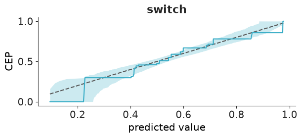
The curve tracks the diagonal through the middle, but at both ends it hugs the edge of the band. Look at the right: above predicted probabilities of about 0.85 it runs along the lower edge - the households the model is most sure about switch a little less often than promised. Suggestive rather than damning; we need a sharper tool.
Binned residuals
Calibration plots show that something is off, not where. Raw residuals $y_i - \hat p_i$ of a binary model are unreadable (two stripes again). Average them within bins of a predictor and they become informative: if the model is right, about 95% of the bin averages should fall inside $\pm 2\sqrt{\bar p(1-\bar p)/n}$.
def plot_binned_residuals(idata, terms, column, ax, n_bins=40):
    p_hat = predict_p(idata, design(wells, terms)).mean(axis=0)
    df = pd.DataFrame({"x": wells[column], "resid": wells.y - p_hat, "var": p_hat * (1 - p_hat)})
    g = df.groupby(pd.qcut(df.x, n_bins, duplicates="drop"), observed=True)
    x, resid, bound = g.x.mean(), g.resid.mean(), 2 * np.sqrt(g["var"].mean() / g.size())
    outside = np.abs(resid) > bound
    ax.plot(x, bound, color="0.6", lw=1)
    ax.plot(x, -bound, color="0.6", lw=1)
    ax.axhline(0, color="k", lw=0.8)
    ax.scatter(x, resid, c=np.where(outside, "C3", "C0"), s=18, zorder=3)
    ax.set(xlabel=column, ylabel="mean residual in bin")
    ax.set_title(f"{int(outside.sum())} of {len(x)} bins outside ± 2 se", loc="right", fontsize=11)


fig, axes = plt.subplots(1, 2, figsize=(11, 3.8), sharey=True)
for ax, column in zip(axes, ["distance", "arsenic"]):
    plot_binned_residuals(idatas["dist + arsenic"], ["dist100", "arsenic"], column, ax)
    ax.set_title("dist + arsenic", loc="left")
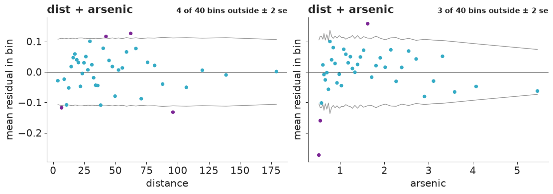
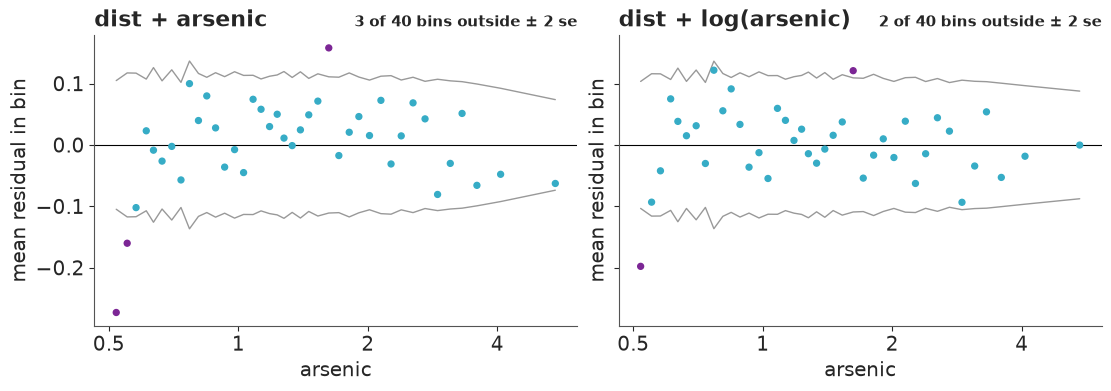
Against distance the residuals look like noise: four bins poke just outside the bounds where chance alone would give about two of 40, but their signs alternate and there is no trend. Against arsenic there is a pattern: the three lowest-arsenic bins are negative, the first of them by 27 percentage points (the model predicts more switching than happens among households barely over the limit), the middle is mostly positive, and five of the six highest bins are negative again. A straight line in arsenic rises too slowly at first and too fast later - the signature of diminishing returns, which is what the very first plot hinted at. The standard fix is to put arsenic on the log scale: going from 0.5 to 1 then matters as much as going from 2 to 4.
idatas["dist + log(arsenic)"], loos["dist + log(arsenic)"] = fit(["dist100", "log_arsenic"], ppc=True)

fig, axes = plt.subplots(1, 2, figsize=(11, 3.8), sharey=True)
for ax, (name, terms) in zip(axes, {"dist + arsenic": ["dist100", "arsenic"], "dist + log(arsenic)": ["dist100", "log_arsenic"]}.items()):
    plot_binned_residuals(idatas[name], terms, "arsenic", ax)
    ax.set_title(name, loc="left")
    ax.set_xscale("log")
    ax.set_xticks([0.5, 1, 2, 4], ["0.5", "1", "2", "4"], minor=False)
    ax.set_xticks([], minor=True)
divergences: 0
az.plot_ppc_pava(idatas["dist + log(arsenic)"]);
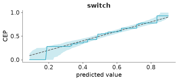
Better, not perfect. The wave in the residuals has gone and the calibration curve now stays inside its band at the top end, but the very first bin - households just above the safety limit - still switches far less than the model expects. (Gelman & Hill suspect a psychological threshold: "barely unsafe" does not feel unsafe. A smooth function of arsenic cannot capture that.)
One more step before comparing everything: education and community association, and whether education changes how people respond to distance.
full_terms = ["dist100", "log_arsenic", "educ4", "assoc", "dist100:educ4"]
idatas["full"], loos["full"] = fit(full_terms)
az.summary(idatas["full"], var_names=["alpha", "beta"], ci_kind="hdi", ci_prob=0.94, round_to=2)
divergences: 0
| mean | sd | hdi94_lb | hdi94_ub | ess_bulk | ess_tail | r_hat | mcse_mean | mcse_sd | |
|---|---|---|---|---|---|---|---|---|---|
| alpha | 0.33 | 0.04 | 0.26 | 0.41 | 5211.42 | 3208.32 | 1.0 | 0.0 | 0.0 |
| beta[dist100] | -1.00 | 0.11 | -1.19 | -0.80 | 4371.85 | 3502.76 | 1.0 | 0.0 | 0.0 |
| beta[log_arsenic] | 0.90 | 0.07 | 0.76 | 1.02 | 4818.07 | 3505.41 | 1.0 | 0.0 | 0.0 |
| beta[educ4] | 0.18 | 0.04 | 0.10 | 0.25 | 6249.08 | 3613.97 | 1.0 | 0.0 | 0.0 |
| beta[assoc] | -0.13 | 0.08 | -0.28 | 0.01 | 5333.35 | 3537.30 | 1.0 | 0.0 | 0.0 |
| beta[dist100:educ4] | 0.38 | 0.10 | 0.18 | 0.56 | 5689.11 | 3407.18 | 1.0 | 0.0 | 0.0 |
8 · Model comparison with PSIS-LOO
We have five models. Binned residuals told us how some of them fail; LOO tells us how much that matters for predicting households we have not seen.
The quantity being estimated is the expected log pointwise predictive density, elpd:
the sum over observations of the log probability the model assigns to $y_i$ when $y_i$
was not used for fitting. Refitting 3020 times is out of the question, so PSIS-LOO
re-weights the draws of the one posterior you have (Pareto-smoothed importance sampling).
That is still the slow step of this notebook (a 4000 x 3020 matrix of weights to smooth per
model), so the fit helper computed it once per model, as az.loo(idata, pointwise=True),
and kept only the result; az.compare accepts those results in place of the DataTrees.
pointwise=True keeps the per-household values, which we will want later. Start by reading
a single model:
loo_full = loos["full"]
loo_full
Computed from 4000 posterior samples and 3020 observations log-likelihood matrix.

         Estimate       SE
elpd_loo -1936.88    17.07
p_loo        6.07        -
------

Pareto k diagnostic values:
                         Count   Pct.
(-Inf, 0.70]   (good)     3020  100.0%
   (0.70, 1]   (bad)         0    0.0%
    (1, Inf)   (very bad)    0    0.0%
How to read this:
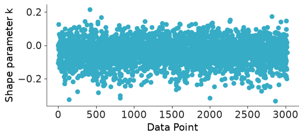
elpd_loois only meaningful relative to another model on the same data. Higher (less negative) is better. For scale: a coin flip would score $3020 \times \log 0.5 \approx -2093$.p_loois the effective number of parameters. Here it is close to the actual count (six coefficients), as it should be for a well-specified model with weak priors. Ap_loofar above the parameter count is a warning sign of misspecification.- Pareto $k$ is a per-observation reliability diagnostic for the importance sampling itself. $k < 0.7$: fine. Larger: that observation is so influential that removing it changes the posterior more than re-weighting can mimic, and the elpd estimate cannot be trusted. With 3020 observations and six parameters no single household is influential, so every $k$ is tiny. (You will meet bad ones in the challenges - they usually point at outliers or at an over-flexible model.)
az.plot_khat(loo_full);
comparison = az.compare(loos, round_to=1)
comparison
| rank | elpd_diff | dse | p_worse | diag_diff | diag_elpd | p | elpd | se | weight | |
|---|---|---|---|---|---|---|---|---|---|---|
| full | 0 | 0.0 | 0.0 | NaN | 6.1 | -1936.9 | 17.1 | 0.9 | ||
| dist + log(arsenic) | 1 | -15.3 | 6.1 | 1.0 | 3.1 | -1952.2 | 16.2 | 0.1 | ||
| dist * arsenic | 2 | -31.2 | 7.7 | 1.0 | 4.4 | -1968.1 | 15.8 | 0.0 | ||
| dist + arsenic | 3 | -31.7 | 7.7 | 1.0 | 3.4 | -1968.6 | 15.6 | 0.0 | ||
| dist | 4 | -103.2 | 14.2 | 1.0 | 1.9 | -2040.0 | 10.4 | 0.0 |
az.plot_compare(comparison);
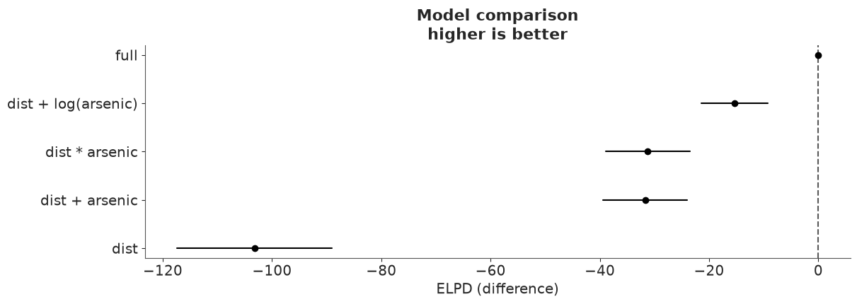
Reading the table:
- Rows are sorted best first.
elpd_diffis each model's elpd minus the best model's;pisp_loo. dseis the standard error of that difference. It is not derived from the twosecolumns: the pointwise elpd values of two models on the same data are highly correlated (a household that is hard to predict is hard for both), so the difference is known far more precisely than either total. Always compareelpd_diffwithdse, never withse.- Rules of thumb: a difference under about 4 is too small to care about whatever its
dse; beyond that, take it seriously when it is severaldsefrom zero.p_worseturns the pair into a probability under a normal approximation - treat it as a rough guide. dseis always relative to the top row. To compare two models further down, callaz.compareon just those two, as we do below.weightis a stacking weight: how to mix the models' predictions to predict best. It is not a posterior probability that the model is true. Near-duplicates share or lose weight arbitrarily.
pairs = [("dist + arsenic", "dist * arsenic"), ("dist + arsenic", "dist + log(arsenic)")]
pd.concat([az.compare({k: loos[k] for k in pair}, round_to=1)[["elpd_diff", "dse", "p"]] for pair in pairs])
| elpd_diff | dse | p | |
|---|---|---|---|
| dist * arsenic | 0.0 | 0.0 | 4.4 |
| dist + arsenic | -0.5 | 1.9 | 3.4 |
| dist + log(arsenic) | 0.0 | 0.0 | 3.1 |
| dist + arsenic | -16.4 | 4.4 | 3.4 |
What all this says:
- Adding arsenic to distance is a huge improvement (about 70 elpd).
- The log transformation beats raw arsenic by about 16 elpd, almost four times its
dse, with the same number of parameters. LOO agrees with the binned residuals. - The distance x arsenic interaction buys nothing: half a unit of elpd, a fraction of
its
dse, for one extra parameter. A coefficient with a 96% posterior probability of being negative can still be irrelevant for prediction. Drop it, unless the interaction itself is the scientific question. - The full model is best: 15 elpd ahead of the runner-up, about 2.5
dse. Convincing, if not overwhelming.
LOO also works pointwise, which makes it a diagnostic rather than only a scoreboard. Where does the log model gain over the linear one?
elpd_lin, elpd_log = loos["dist + arsenic"].elpd_i, loos["dist + log(arsenic)"].elpd_i
gain = pd.DataFrame({"arsenic": wells.arsenic.values, "gain": (elpd_log - elpd_lin).values})
by_bin = gain.groupby(pd.qcut(gain.arsenic, 12), observed=True).agg(arsenic=("arsenic", "mean"), gain=("gain", "sum"))

fig, ax = plt.subplots(figsize=(7, 3.8))
ax.bar(range(len(by_bin)), by_bin.gain, color=np.where(by_bin.gain > 0, "C0", "C3"))
ax.set_xticks(range(len(by_bin)), by_bin.arsenic.round(2), rotation=45)
ax.axhline(0, color="k", lw=0.8)
ax.set(xlabel="mean arsenic level in bin (12 equal-count bins)", ylabel="elpd gained by log(arsenic)");
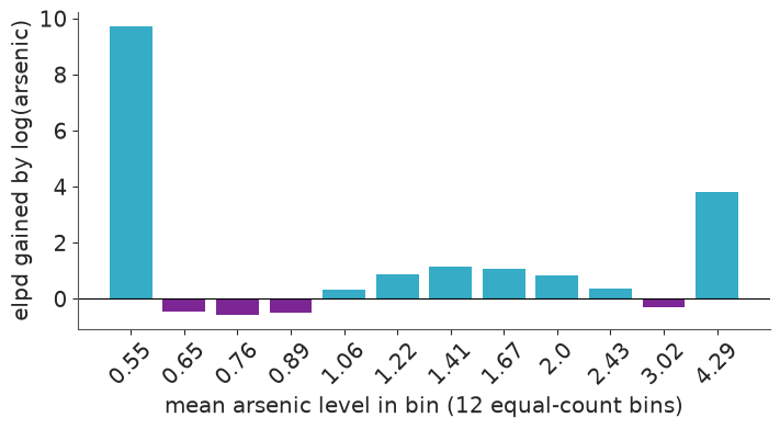
Most of the gain - roughly 13 of the 16 units - comes from the two end bins: the barely-unsafe wells and the most contaminated ones, exactly where the binned residuals of the linear model were negative. In between, each bin moves by about one unit or less in either direction: there the two models predict almost equally well.
9 · Answer the planner
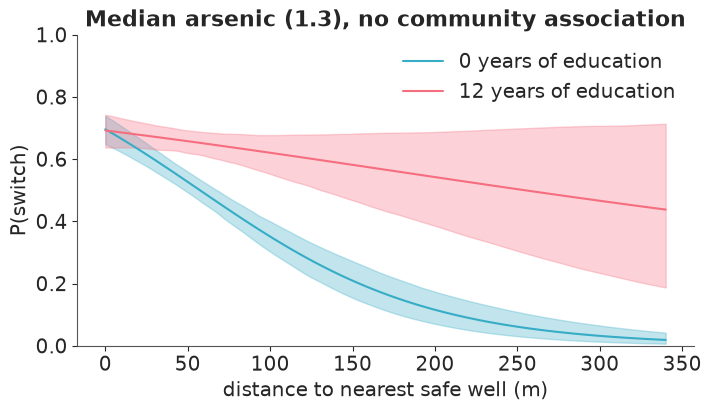
Back to probabilities, with the best model. The interaction with education makes "the effect of distance" depend on who you ask, which is precisely the situation average predictive differences are built for.
report(average_predictive_difference(idatas["full"], full_terms, "distance", 0, 100), "distance: next door -> 100 m away")
report(average_predictive_difference(idatas["full"], full_terms, "arsenic", 0.5, 1.0), "arsenic: 0.5 -> 1.0")
report(average_predictive_difference(idatas["full"], full_terms, "arsenic", 1.0, 2.0), "arsenic: 1.0 -> 2.0")
report(average_predictive_difference(idatas["full"], full_terms, "education", 0, 12), "education: none -> 12 years")
report(average_predictive_difference(idatas["full"], full_terms, "association", "no", "yes"), "community association: no -> yes")
distance: next door -> 100 m away          -0.222   94% interval [-0.267, -0.179]
arsenic: 0.5 -> 1.0                        +0.146   94% interval [+0.126, +0.164]
arsenic: 1.0 -> 2.0                        +0.143   94% interval [+0.123, +0.161]
education: none -> 12 years                +0.118   94% interval [+0.068, +0.165]
community association: no -> yes           -0.031   94% interval [-0.066, +0.002]
fig, ax = plt.subplots(figsize=(7, 4))
for color, years in zip(["C0", "C1"], [0, 12]):
    g = prepare(grid.assign(arsenic=wells.arsenic.median(), education=years))
    p = predict_p(idatas["full"], design(g, full_terms))
    ax.fill_between(g.distance, *np.quantile(p, [0.03, 0.97], axis=0), color=color, alpha=0.3)
    ax.plot(g.distance, p.mean(axis=0), color=color, label=f"{years} years of education")
ax.set(xlabel="distance to nearest safe well (m)", ylabel="P(switch)", ylim=(0, 1),
       title=f"Median arsenic ({wells.arsenic.median():.1f}), no community association")
ax.legend();
For a planner:
- Having to walk 100 m instead of next door lowers the switching probability by about 22 percentage points on average. The deterrent is strongest among the least educated; with 12 years of schooling the curve is much flatter (and, with few such households far from a safe well, much less certain). New safe wells are worth most where the nearest alternative is far away and education is low.
- The choice of scale for arsenic was not a technicality. The linear model put the effect of going from 0.5 to 1.0 at under 6 percentage points; the log model says 15 - the same as going from 1.0 to 2.0. The better-fitting model tells a different story about who responds to information.
- The surprise is community association: if anything its members switch less, though the interval reaches zero.
A caution the model cannot give you: this is an observational survey. "Setting distance to 0" in a computation is not the same as drilling a well next door; calling a predictive difference causal takes assumptions that no amount of LOO can check.
Try it yourself
- Refit the distance-only model with the
Normal(0, 10)priors on all 3020 households and then on a random subsample of 30. How much do the two priors disagree in each case? Plot the posterior curves for both. - The binned residuals still show too few switchers just above the safety limit. Add a term
that lets the model treat "barely unsafe" wells differently (for example an indicator for
arsenic < 0.6, or a spline in log arsenic) and compare withaz.compare. Is the improvement worth a parameter nobody can interpret? - Swap the link: replace
logit_p=etawithp=pm.math.invprobit(eta). Coefficients shrink by a factor of about 1.6 - do the average predictive differences change? Does LOO care?
Next: challenge C03 moves from binary outcomes to counts, and gives LOO's Pareto-$k$ diagnostic real work to do.