Time-to-event data looks like a regression problem until you notice that for many rows the event has not happened yet. The study ended, the customer is still subscribed, the machine is still running. Those rows are not missing and they are not events: they are lower bounds. This notebook shows what goes wrong when you pretend otherwise, and how little code it takes in PyMC to do it properly.
import warnings

import arviz as az
import matplotlib.pyplot as plt
import numpy as np
import pandas as pd
import pymc as pm
from matplotlib.lines import Line2D
from scipy import stats

from pymc_challenges import data

RANDOM_SEED = 44
rng = np.random.default_rng(RANDOM_SEED)
az.style.use("arviz-variat")
1 · Question and data
How long do women survive after a mastectomy, and how much shorter is survival when the
cancer had metastasized? Each row is one patient: time is months of follow-up, event is
True if she died at that time and False if she was still alive when last seen.
data.describe("mastectomy")
df = data.load("mastectomy")
df["group"] = np.where(df.metastasized == "yes", "metastasized", "not metastasized")
df.groupby("group").agg(
    patients=("time", "size"), deaths=("event", "sum"), mean_followup=("time", "mean")
).round(1)
mastectomy: Months of follow-up, death indicator and metastasis status for 44 women.
  source: Survival of breast-cancer patients after mastectomy, via R package `HSAUR`.
  url:    https://raw.githubusercontent.com/pymc-devs/pymc-examples/main/examples/data/mastectomy.csv
| patients | deaths | mean_followup | |
|---|---|---|---|
| group | |||
| metastasized | 32 | 21 | 83.4 |
| not metastasized | 12 | 5 | 131.8 |
Only 26 of the 44 women died during the study. For the other 18 all we know is that they
survived at least time months. That is right-censoring. One line per patient makes
the structure obvious:
order = df.sort_values(["group", "time"]).reset_index(drop=True)
colors = order.group.map({"not metastasized": "C0", "metastasized": "C1"})

fig, ax = plt.subplots(figsize=(8, 7))
ax.hlines(order.index, 0, order.time, color=colors, lw=1.5)
died = order[order.event]
alive = order[~order.event]
ax.scatter(died.time, died.index, marker="x", color="k", zorder=3, label="died")
ax.scatter(alive.time, alive.index, marker=">", facecolor="w", edgecolor="k", zorder=3,
           label="alive when last seen (censored)")
for name, color in [("not metastasized", "C0"), ("metastasized", "C1")]:
    ax.plot([], [], color=color, lw=1.5, label=name)
ax.set(xlabel="months since mastectomy", ylabel="patient", yticks=[])
ax.legend(loc="lower right");
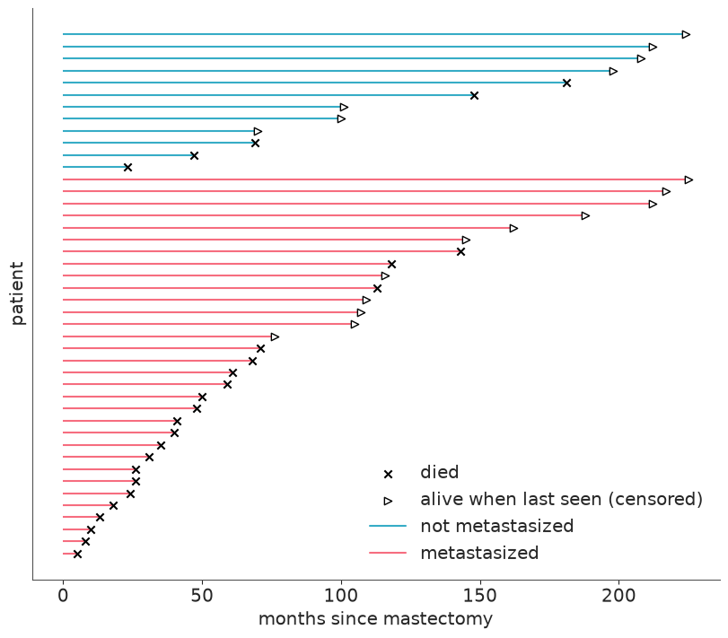
Notice who is censored: mostly the long lines. Censored patients are not a random subset, they are disproportionately the long survivors. Hold that thought.
2 · A model-free benchmark: Kaplan-Meier
The Kaplan-Meier (KM) estimator is the empirical survival function that respects censoring. At each death time $t_j$ with $d_j$ deaths among the $n_j$ patients still under observation, survival is multiplied by $(1 - d_j / n_j)$. Censored patients count in the denominator $n_j$ for as long as they were observed and then silently leave. Ten lines of NumPy:
def kaplan_meier(time, event):
    """Kaplan-Meier estimate. Returns step-function knots (t, S), starting at (0, 1)."""
    time, event = np.asarray(time, dtype=float), np.asarray(event, dtype=bool)
    t_event = np.unique(time[event])
    at_risk = np.array([(time >= t).sum() for t in t_event])
    deaths = np.array([((time == t) & event).sum() for t in t_event])
    surv = np.cumprod(1 - deaths / at_risk)
    # extend the last step to the end of follow-up
    return np.r_[0, t_event, time.max()], np.r_[1, surv, surv[-1]]


GROUP_COLORS = {"not metastasized": "C0", "metastasized": "C1"}


def plot_km(ax):
    for name, grp in df.groupby("group"):
        ax.step(*kaplan_meier(grp.time, grp.event), where="post", color=GROUP_COLORS[name], lw=2,
                label=f"KM, {name}")
    ax.set(xlabel="months since mastectomy", ylabel="S(t) = P(alive at t)", ylim=(0, 1.02))


fig, ax = plt.subplots()
plot_km(ax)
ax.axhline(0.5, color="k", ls=":", lw=1)
ax.legend();
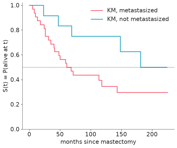
The metastasized group (red) reaches $S = 0.5$ after roughly 60-70 months. The other group only touches 0.5 with its very last observed death, at 181 months, when just five women were still under observation - a "median" that rests on a single event. KM also cannot extrapolate beyond the last follow-up, has no smooth hazard, and offers no direct measure of the group difference with uncertainty. That is what a parametric model buys - at the price of assumptions we will have to check against this very curve.
3 · The likelihood of "not yet"
Let $T$ be the survival time with density $f$ and survival function $S(t) = P(T > t)$.
- A patient who died at $t_i$ contributes $f(t_i)$, as usual.
- A patient censored at $t_i$ contributes $P(T > t_i) = S(t_i)$: we saw that the event had not happened by $t_i$, nothing more.
pm.Censored(name, dist, lower, upper, observed) implements exactly this: an observed value
equal to the bound upper contributes $P(T \ge \text{upper})$, anything below it contributes
the density. lower and upper can be arrays, one bound per observation, which is the
whole trick:
- censored row:
upper= her follow-up time (so the observed value sits on the bound); - death:
upper= $\infty$ (no bound, ordinary density).
t = df.time.to_numpy(dtype=float)
event = df.event.to_numpy()
metastasized = (df.metastasized == "yes").to_numpy(dtype=int)
upper = np.where(event, np.inf, t)
X_MEAN = metastasized.mean()  # used to centre the covariate, see section 4
Do not take the idiom on trust. pm.logp lets us check it against SciPy for an arbitrary
Weibull: deaths should get logpdf, censored rows logsf (log survival function).
censored_dist = pm.Censored.dist(pm.Weibull.dist(alpha=1.5, beta=100.0), lower=None, upper=upper)
logp_pymc = pm.logp(censored_dist, t).eval()
logp_scipy = np.where(
    event,
    stats.weibull_min.logpdf(t, 1.5, scale=100.0),
    stats.weibull_min.logsf(t, 1.5, scale=100.0),
)
print("pm.Censored matches f(t) for deaths and S(t) for censored rows:", np.allclose(logp_pymc, logp_scipy))
pm.Censored matches f(t) for deaths and S(t) for censored rows: True
4 · An exponential AFT model
Start with the simplest survival distribution, the Exponential (constant hazard), and let its scale depend on metastasis:
$$ T_i \sim \text{Exponential}(\text{scale} = \lambda_i), \qquad \log \lambda_i = \alpha + \beta\,(\text{metastasized}_i - \bar{x}) $$
This is an accelerated failure time (AFT) model: the covariate stretches or shrinks the time axis. $e^{\beta}$ is a time ratio - if $e^\beta = 0.5$, every quantile of survival time (median included) is halved for metastasized patients, as if their clock ran twice as fast.
Why centre a 0/1 covariate? Only 12 women are in the reference group. With the raw indicator, $\alpha$ would be informed by those 12 alone and every change in $\alpha$ would have to be undone by $\beta$ for the other 32, so the two end up strongly correlated in the posterior and the sampler works harder for the same answer. Subtracting the mean $\bar{x}$ (the share of metastasized patients) makes $\alpha$ the log scale of an "average" patient. $\beta$ and its interpretation are untouched. Section 6 puts numbers on the difference.
Priors. Normal(4.5, 1.5) on $\alpha$ puts the typical median survival
($\lambda \ln 2$) around 5 years, with a 94% range from a few months to many decades.
$\beta \sim$ Normal(0, 1) says the time ratio is most likely between 1/7 and 7 and does
not presume the sign. We write one function so that the very same model can later be
fitted to mangled versions of the data.
def fit_aft(family, time, upper, x, beta_sd=1.0, alpha_sd=1.5, prior_only=False, centre=True):
    """Censored AFT model. family is "exponential" or "weibull"."""
    with pm.Model(coords={"obs": np.arange(len(time))}) as model:
        upper_ = pm.Data("upper", upper, dims="obs")
        alpha = pm.Normal("alpha", 4.5, alpha_sd)
        beta = pm.Normal("beta", 0, beta_sd)
        scale = pm.math.exp(alpha + beta * (x - X_MEAN if centre else x))
        if family == "exponential":
            dist = pm.Exponential.dist(scale=scale)
        else:
            k = pm.LogNormal("k", 0, 0.5)
            dist = pm.Weibull.dist(alpha=k, beta=scale)
        pm.Deterministic("time_ratio", pm.math.exp(beta))
        pm.Censored("time", dist, lower=None, upper=upper_, observed=time, dims="obs")
        if prior_only:
            return model, pm.sample_prior_predictive(1000, random_seed=RANDOM_SEED)
        idata = pm.sample(random_seed=RANDOM_SEED)
    return model, idata


_, exp_prior = fit_aft("exponential", t, upper, metastasized, prior_only=True)

prior = az.extract(exp_prior, group="prior")
prior_median = np.exp(prior["alpha"].values) * np.log(2)
print("prior median survival of a typical patient, months (3%, 50%, 97%):",
      np.quantile(prior_median, [0.03, 0.5, 0.97]).round(0))

fig, ax = plt.subplots()
grid = np.linspace(0, 240, 200)
ax.plot(grid, np.exp(-grid[:, None] / np.exp(prior["alpha"].values[:60])), color="C0", alpha=0.3)
ax.set(xlabel="months", ylabel="S(t)", title="Survival curves implied by the prior (typical patient)");
prior median survival of a typical patient, months (3%, 50%, 97%): [ 4. 62. 1073.]
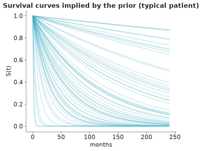
From "almost everybody dies within the first year" to "nearly nine in ten are alive after twenty": wide, but every curve is something that could happen after cancer surgery. Now fit.
exp_model, exp_idata = fit_aft("exponential", t, upper, metastasized)

print("divergences:", int(exp_idata.sample_stats["diverging"].sum()))
az.summary(exp_idata, ci_kind="hdi", ci_prob=0.94, round_to=2)
divergences: 0
| mean | sd | hdi94_lb | hdi94_ub | ess_bulk | ess_tail | r_hat | mcse_mean | mcse_sd | |
|---|---|---|---|---|---|---|---|---|---|
| alpha | 5.11 | 0.20 | 4.74 | 5.49 | 4035.14 | 2496.64 | 1.0 | 0.00 | 0.00 |
| beta | -0.79 | 0.44 | -1.61 | 0.02 | 3742.69 | 2275.52 | 1.0 | 0.01 | 0.01 |
| time_ratio | 0.50 | 0.22 | 0.14 | 0.89 | 3742.69 | 2275.52 | 1.0 | 0.00 | 0.00 |
Clean diagnostics. Before interpreting, the promised demonstration.
5 · What happens if you ignore censoring
Two tempting shortcuts, each fitted with the same model and priors:
- drop: keep only the 26 women whose death was observed ("we only know the true time for them");
- pretend: keep everyone but treat censored follow-up times as death times.
no_bound = np.full(len(t), np.inf)
_, drop_idata = fit_aft("exponential", t[event], no_bound[event], metastasized[event])
_, pretend_idata = fit_aft("exponential", t, no_bound, metastasized)
def scale_draws(post, x):
    """Posterior draws of the scale parameter for metastasis indicator x (0 or 1)."""
    return np.exp(post["alpha"].values + post["beta"].values * (x - X_MEAN))


def median_survival(idata):
    """Posterior draws of median survival (months) per group, for either family."""
    post = az.extract(idata)
    k = post["k"].values if "k" in post else 1.0
    return {
        name: scale_draws(post, x) * np.log(2) ** (1 / k)
        for name, x in [("not metastasized", 0), ("metastasized", 1)]
    }


rows = {}
for label, idata in [("censored (correct)", exp_idata), ("drop censored rows", drop_idata),
                     ("pretend censored = died", pretend_idata)]:
    for name, draws in median_survival(idata).items():
        lo, mid, hi = np.quantile(draws, [0.03, 0.5, 0.97])
        rows[(label, name)] = {"median survival (months)": mid, "3%": lo, "97%": hi}
bias_table = pd.DataFrame(rows).T.round(0)
bias_table
| median survival (months) | 3% | 97% | ||
|---|---|---|---|---|
| censored (correct) | not metastasized | 199.0 | 101.0 | 455.0 |
| metastasized | 92.0 | 63.0 | 142.0 | |
| drop censored rows | not metastasized | 61.0 | 32.0 | 141.0 |
| metastasized | 35.0 | 24.0 | 53.0 | |
| pretend censored = died | not metastasized | 90.0 | 56.0 | 155.0 |
| metastasized | 59.0 | 43.0 | 83.0 |
fits = [("censored likelihood", exp_idata, "-"), ("drop censored rows", drop_idata, ":"),
        ("pretend censored = died", pretend_idata, "--")]

fig, ax = plt.subplots()
plot_km(ax)
for label, idata, ls in fits:
    post = az.extract(idata)
    for x, color in [(0, "C0"), (1, "C1")]:
        ax.plot(grid, np.exp(-grid[:, None] / scale_draws(post, x)).mean(axis=1), color=color, ls=ls)
handles = [Line2D([], [], color="k", lw=2, drawstyle="steps-post", label="Kaplan-Meier")]
handles += [Line2D([], [], color="k", ls=ls, label=label) for label, _, ls in fits]
ax.legend(handles=handles, fontsize=9, title="colours as above");
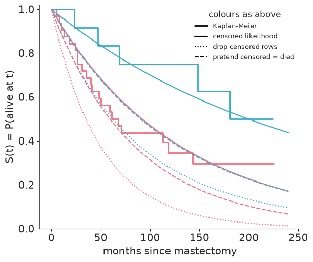
Both shortcuts are badly pessimistic, and the posterior intervals give no warning:
- Dropping censored rows throws away precisely the long survivors (remember the line plot). The estimated median survival falls to 30-40% of the correct one, and the dotted curves sit far below the Kaplan-Meier steps.
- Pretending is milder but biased the same way - median survival comes out at roughly 45-65% of the correct value - because every "she was alive at 150 months" is recorded as "she died at 150 months".
Only the censored likelihood (solid) tracks the KM curves. The bias grows with the censored fraction, which is why it is worst for the non-metastasized group (7 of 12 censored). It is also as large as the effect we are trying to measure: the "pretend" curve for women without metastasis (dashed blue) lies almost exactly on top of the correct curve for women with it (solid red).
6 · Is the hazard constant? A Weibull model
The Exponential has a constant hazard: the risk of dying next month is the same 6 months and 10 years after surgery. The Weibull adds a shape $k$:
$$S(t) = \exp\!\big(-(t/\lambda)^k\big), \qquad h(t) \propto t^{\,k-1}$$
$k < 1$ means the hazard falls with time, $k > 1$ that it rises, and $k = 1$ is the
Exponential. In PyMC's pm.Weibull(alpha, beta) the shape is alpha and the scale is beta
(do not confuse them with our regression coefficients). The AFT reading of $e^\beta$ as a
time ratio is unchanged. The prior LogNormal(0, 0.5) centres $k$ on 1 and covers 0.4-2.6.
wei_model, wei_idata = fit_aft("weibull", t, upper, metastasized)

print("divergences:", int(wei_idata.sample_stats["diverging"].sum()))
az.summary(wei_idata, ci_kind="hdi", ci_prob=0.94, round_to=2)
divergences: 0
| mean | sd | hdi94_lb | hdi94_ub | ess_bulk | ess_tail | r_hat | mcse_mean | mcse_sd | |
|---|---|---|---|---|---|---|---|---|---|
| alpha | 5.15 | 0.23 | 4.73 | 5.58 | 3004.01 | 2389.75 | 1.0 | 0.00 | 0.00 |
| beta | -0.78 | 0.46 | -1.60 | 0.15 | 3673.78 | 2581.21 | 1.0 | 0.01 | 0.01 |
| k | 0.91 | 0.14 | 0.66 | 1.19 | 3241.86 | 2742.84 | 1.0 | 0.00 | 0.00 |
| time_ratio | 0.51 | 0.24 | 0.14 | 0.94 | 3673.78 | 2581.21 | 1.0 | 0.00 | 0.01 |
az.plot_rank(wei_idata, var_names=["alpha", "beta", "k"]);

r_hat of 1.00, ESS in the thousands, and the uniformity test printed in each rank plot
flags nothing. The shape $k$ is estimated a little below 1 with an interval that
comfortably includes 1: no evidence against a constant hazard, which the formal comparison
below confirms.
Aside: what centring bought us
The same model with the raw 0/1 indicator, for comparison:
_, raw_idata = fit_aft("weibull", t, upper, metastasized, centre=False)

centring = {}
for label, idata in [("centred", wei_idata), ("raw 0/1 indicator", raw_idata)]:
    post = az.extract(idata)
    ess = az.ess(idata, var_names=["alpha", "beta"])
    centring[label] = {
        "corr(alpha, beta)": np.corrcoef(post["alpha"], post["beta"])[0, 1],
        "ess_bulk alpha": float(ess["alpha"]),
        "ess_bulk beta": float(ess["beta"]),
    }
pd.DataFrame(centring).T.round(2)
| corr(alpha, beta) | ess_bulk alpha | ess_bulk beta | |
|---|---|---|---|
| centred | -0.07 | 3004.01 | 3673.78 |
| raw 0/1 indicator | -0.83 | 1227.73 | 1227.30 |
Uncentred, $\alpha$ and $\beta$ have a posterior correlation of about -0.8 and the same 4000
draws are worth well under half as many effective draws. Nothing breaks in a model this
small - r_hat is still fine - but the habit pays off in larger regressions, where correlated
intercepts and slopes are a common cause of slow sampling.
Survival curves with uncertainty
$S(t)$ is a deterministic function of the parameters, so each posterior draw gives a whole curve; quantiles across draws give the band.
def survival_curves(idata, x, grid):
    """Array (draws, len(grid)) of S(t) for a patient with metastasis indicator x."""
    post = az.extract(idata)
    k = post["k"].values[:, None] if "k" in post else 1.0
    scale = scale_draws(post, x)[:, None]
    return np.exp(-((grid / scale) ** k))


fig, ax = plt.subplots()
plot_km(ax)
for x, color, name in [(0, "C0", "not metastasized"), (1, "C1", "metastasized")]:
    curves = survival_curves(wei_idata, x, grid)
    lo, hi = np.quantile(curves, [0.03, 0.97], axis=0)
    ax.fill_between(grid, lo, hi, color=color, alpha=0.25)
    ax.plot(grid, curves.mean(axis=0), color=color, label=f"Weibull, {name}")
ax.legend(fontsize=9);
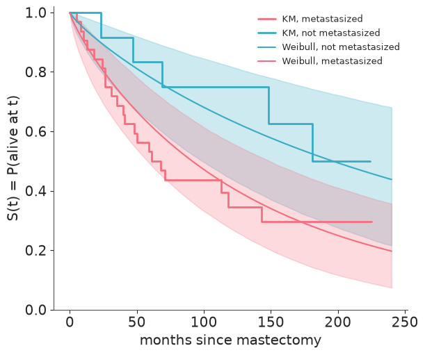
The KM steps stay inside the 94% bands, except that the non-metastasized curve starts a touch above its band: nobody in that group of 12 died in the first 23 months, which a handful of patients can easily do by chance. The bands are wide - this is what 44 patients and 26 deaths can tell you - and widest for the small non-metastasized group, whose curve is informed by only 5 deaths.
A posterior predictive check made for censored data
A standard PPC compares observed and replicated outcomes, but our observed time mixes
deaths with censoring times, so a density overlay would compare apples with oranges.
az.plot_ppc_censored does the right thing: it draws the Kaplan-Meier curve of the
observed data against the survival curves of replicated datasets. It needs three things:
- Uncensored replicated times. Draws from
pm.Censoredare clipped atupper, so we first lift the bound - this is whyupperwas registered withpm.Data. - An event indicator (1 = event, 0 = censored) in
constant_data, under the same name as the observed variable. extrapolation_factor=None. The default (1.2) discards replicated times beyond 1.2x the longest follow-up and renormalises, which drags every replicated curve down to zero at that point. With heavy censoring that makes a good model look bad. We keep all draws and simply zoom the axis instead.
with wei_model, warnings.catch_warnings():
    # PyTensor compares old and new data values and grumbles about inf - inf; harmless
    warnings.simplefilter("ignore", RuntimeWarning)
    pm.set_data({"upper": no_bound})
    wei_ppc = pm.sample_posterior_predictive(wei_idata, random_seed=RANDOM_SEED)
    pm.set_data({"upper": upper})

wei_ppc["constant_data"] = wei_ppc["constant_data"].to_dataset().assign(time=("obs", event.astype(int)))
az.plot_ppc_censored(wei_ppc, var_names="time", num_samples=100, extrapolation_factor=None)
plt.gcf().set_size_inches(7, 4)
plt.gcf().axes[0].set(xlim=(0, 240), xlabel="months since mastectomy");
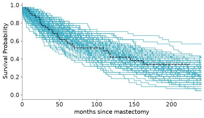
The observed KM curve (dashed, both groups pooled) runs through the middle of the replicated curves. Nothing here or in the per-group plot above argues against the Weibull AFT model.
7 · Interpret: time ratio and median survival
post = az.extract(wei_idata)
time_ratio = post["time_ratio"].values
print(f"time ratio exp(beta): median {np.median(time_ratio):.2f}, "
      f"94% interval {np.quantile(time_ratio, [0.03, 0.97]).round(2)}")
print(f"P(metastasis shortens survival) = {(time_ratio < 1).mean():.2f}")

medians = median_survival(wei_idata)
for name, draws in medians.items():
    print(f"median survival, {name:<17}: {np.median(draws):4.0f} months, "
          f"94% interval {np.quantile(draws, [0.03, 0.97]).round(0)}, "
          f"P(beyond end of follow-up) = {(draws > t.max()).mean():.2f}")
time ratio exp(beta): median 0.46, 94% interval [0.18 1.05]
P(metastasis shortens survival) = 0.96
median survival, not metastasized :  197 months, 94% interval [ 99. 462.], P(beyond end of follow-up) = 0.36
median survival, metastasized     :   91 months, 94% interval [ 58. 149.], P(beyond end of follow-up) = 0.00
fig, ax = plt.subplots()
bins = np.geomspace(20, 3000, 60)
for name, draws in medians.items():
    ax.hist(draws, bins=bins, color=GROUP_COLORS[name], alpha=0.6, label=name)
ax.axvline(t.max(), color="k", ls=":", label="end of follow-up")
ax.set(xscale="log", xlabel="median survival (months, log scale)", yticks=[],
       title="Posterior of median survival")
ax.legend();
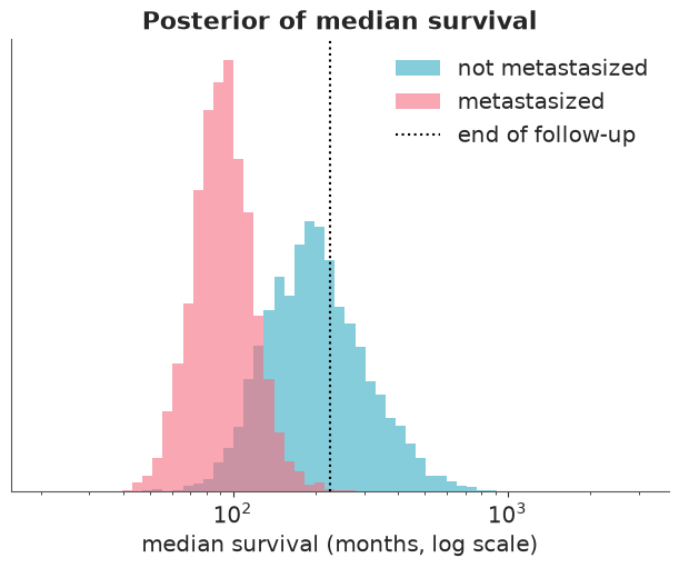
Metastasized cancer roughly halves survival time, and the posterior probability that it shortens survival at all is high (about 0.96) but not overwhelming. The median survival of metastasized patients is pinned down reasonably well because we watched more than half of them die. For the other group more than a third of the posterior lies beyond the end of follow-up: that number is an extrapolation resting on the Weibull shape, not on data. Kaplan-Meier's median rested on a single death; the parametric model answers with a (rightly) huge interval.
8 · Exponential or Weibull?
LOO works unchanged: the pointwise log-likelihood of a censored row is simply $\log S(t_i)$.
with exp_model:
    pm.compute_log_likelihood(exp_idata, progressbar=False)
with wei_model:
    pm.compute_log_likelihood(wei_idata, progressbar=False)

az.compare({"exponential": exp_idata, "weibull": wei_idata})
| rank | elpd_diff | dse | p_worse | diag_diff | diag_elpd | p | elpd | se | weight | |
|---|---|---|---|---|---|---|---|---|---|---|
| exponential | 0 | 0.0 | 0.00 | NaN | 2.1 | -160.0 | 15.0 | 1.0 | ||
| weibull | 1 | -0.5 | 0.45 | 0.86 | N < 100 | 2.3 | -160.0 | 15.0 | 0.0 |
Less than one elpd point apart. The simpler Exponential is marginally ahead because the
Weibull's extra parameter buys nothing, but a gap this small (note ArviZ's N < 100 flag
on the difference) is no reason to prefer either. With 26 events there is no information to
distinguish $k = 0.9$ from $k = 1$. We keep the Weibull for reporting, because its intervals
honestly include our ignorance about the hazard shape.
9 · Small data: how much is the prior doing?
With 26 deaths the prior cannot be an afterthought. az.psense_summary perturbs the prior
and the likelihood by raising each to a power slightly different from 1 and measures how
far the posterior moves (it needs the log_prior and log_likelihood groups). Values above
0.05 flag sensitivity.
with wei_model:
    pm.stats.compute_log_prior(wei_idata, progressbar=False)

az.psense_summary(wei_idata, var_names=["alpha", "beta", "k"])
| prior | likelihood | diagnosis | |
|---|---|---|---|
| alpha | 0.019 | 0.103 | ✓ |
| beta | 0.074 | 0.094 | potential prior-data conflict |
| k | 0.011 | 0.071 | ✓ |
beta - the one parameter the clinical question is about - is flagged: its posterior
responds to the prior and to the likelihood. ArviZ words this as a "potential prior-data
conflict", but read it for what the numbers say: with 12 patients in one group, a
Normal(0, 1) prior is informative enough to matter. alpha and k are not
prior-sensitive. A diagnostic flag is a prompt to look, so look:
refit with a much tighter and a much wider prior on $\beta$ and compare the quantity we care about.
sens = {}
for beta_sd in [0.3, 1.0, 5.0]:
    idata = wei_idata if beta_sd == 1.0 else fit_aft("weibull", t, upper, metastasized, beta_sd=beta_sd)[1]
    ratio = az.extract(idata, var_names="time_ratio").values
    lo, mid, hi = np.quantile(ratio, [0.03, 0.5, 0.97])
    sens[f"beta ~ Normal(0, {beta_sd})"] = {
        "time ratio (median)": mid, "3%": lo, "97%": hi, "P(ratio < 1)": (ratio < 1).mean()
    }
pd.DataFrame(sens).T.round(2)
| time ratio (median) | 3% | 97% | P(ratio < 1) | |
|---|---|---|---|---|
| beta ~ Normal(0, 0.3) | 0.77 | 0.47 | 1.24 | 0.84 |
| beta ~ Normal(0, 1.0) | 0.46 | 0.18 | 1.05 | 0.96 |
| beta ~ Normal(0, 5.0) | 0.36 | 0.09 | 0.96 | 0.97 |
Read the table from the middle row outwards. A sceptical prior (sd = 0.3, "metastasis
changes survival time by at most a factor of two or so") pulls the time ratio clearly
towards 1 and leaves real doubt about the sign; a nearly flat prior (sd = 5) lets the
ratio drift further from 1 than our default. The direction of the effect is the same
under every prior, its size ranges from roughly a quarter off to almost two thirds off
survival time. That is the honest summary of a 44-patient study, and it is the reason a
Bayesian analysis of small survival data should always state its priors and show this table.
Try it yourself
- Replace the Weibull with a log-normal AFT model (
pm.LogNormal.dist(mu=alpha + beta * x, sigma=sigma)). Its hazard rises and then falls. Does LOO prefer it? Do the median survival estimates for the non-metastasized group change, and why is that group so sensitive to the choice of family? - Let the Weibull shape differ by group (
kwithdims="group"). The KM curves hint that the groups might differ in hazard shape - is there enough data to tell? - Artificially censor the data further: pretend the study had stopped at 100 months (every
time > 100becomes a censored observation at 100). How much wider do the posteriors of the time ratio and of median survival become, and how much worse do the two naive shortcuts of section 5 get?
Next: challenge C04 applies all of this to 7,000 telecom customers, most of whom have not churned yet.