Splines and polynomials make you choose a functional form. A Gaussian process lets you say something weaker and more honest: "the function is smooth, it varies by about this much, and it changes on roughly this timescale". That is a prior over functions, and this notebook builds one up from scratch, fits it exactly, then fits it fast, and finally uses the speed to buy a better model.
import time

import arviz as az
import matplotlib.pyplot as plt
import numpy as np
import pandas as pd
import preliz as pz
import pymc as pm
from pymc.model.transform.optimization import freeze_dims_and_data

from pymc_challenges import data

RANDOM_SEED = 1985
rng = np.random.default_rng(RANDOM_SEED)
az.style.use("arviz-variat")

print(f"PyMC {pm.__version__}, ArviZ {az.__version__}, PreliZ {pz.__version__}")
PyMC 6.3.2, ArviZ 1.3.0, PreliZ 0.28.0
1 · Question and data
A dummy's head is fitted with an accelerometer and the motorcycle is crashed into a wall. What is the acceleration curve, and how variable are readings around it? Helmet designers care about both: the curve is the typical load, the scatter is what the helmet must survive.
data.describe("mcycle")
mcycle = data.load("mcycle")
mcycle.describe().round(1)
mcycle: Head acceleration (g) against time after impact (ms), 133 readings.
  source: Silverman (1985), simulated motorcycle crash experiment, via R package `MASS`.
  url:    https://vincentarelbundock.github.io/Rdatasets/csv/MASS/mcycle.csv
| times | accel | |
|---|---|---|
| count | 133.0 | 133.0 |
| mean | 25.2 | -25.5 |
| std | 13.1 | 48.3 |
| min | 2.4 | -134.0 |
| 25% | 15.6 | -54.9 |
| 50% | 23.4 | -13.3 |
| 75% | 34.8 | 0.0 |
| max | 57.6 | 75.0 |
fig, ax = plt.subplots(figsize=(8, 4))
ax.scatter(mcycle.times, mcycle.accel, s=14, color="k")
ax.set(xlabel="time after impact (ms)", ylabel="head acceleration (g)");
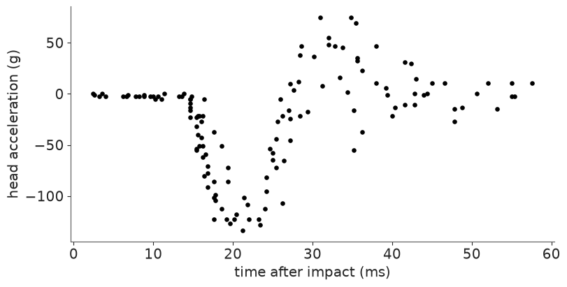
Three things to notice:
- The curve is flat, plunges to about -120 g, rebounds and settles. No low-order polynomial does that.
- The scatter is not constant. Before ~13 ms the readings sit within a few g of zero; after the impact they are spread over 50 g or more. Keep this in mind - the first models below ignore it, and section 7 is about what that costs.
- Several times carry more than one reading, which a GP handles without fuss.
We divide acceleration by its standard deviation so that "1" is a typical swing, but we do not centre it: 0 g is the physically meaningful baseline before the impact, and a GP with a zero mean function returns to 0 when it has no data - exactly what we want here. Time stays in milliseconds so that the lengthscale is readable.
t = mcycle.times.to_numpy()
ACCEL_SD = mcycle.accel.std()
y = mcycle.accel.to_numpy() / ACCEL_SD

t_grid = np.linspace(0, 60, 200)
print(f"1 unit of y = {ACCEL_SD:.1f} g;  {len(t)} readings at {len(np.unique(t))} distinct times")
1 unit of y = 48.3 g; 133 readings at 94 distinct times
2 · A GP is a prior over functions
A Gaussian process says: for any set of inputs $t_1, \dots, t_n$, the function values are jointly Normal,
$$f(t_1), \dots, f(t_n) \sim \text{MvNormal}\big(0,\ K\big), \qquad K_{ij} = k(t_i, t_j).$$
All the modelling is in the kernel $k$: it says how strongly two function values are correlated as a function of how far apart their inputs are. We will use the Matérn 5/2 kernel
$$k(t, t') = \eta^2 \Big(1 + \tfrac{\sqrt5\, r}{\ell} + \tfrac{5 r^2}{3 \ell^2}\Big) \exp\!\Big(-\tfrac{\sqrt5\, r}{\ell}\Big), \qquad r = |t - t'|,$$
which gives twice-differentiable functions - smooth, but not as unrealistically smooth as the squared-exponential. It has two hyperparameters:
- the amplitude $\eta$: the prior standard deviation of $f$ at any point;
- the lengthscale $\ell$: how far you must move before the function "forgets" where it was.
The quickest way to understand them is to draw functions. A PyMC covariance object is
callable: cov(X) builds the matrix symbolically and .eval() gives NumPy.
fig, axes = plt.subplots(1, 3, figsize=(12, 3.2), sharey=True)
for ax, ls in zip(axes, [2, 8, 30]):
    cov = pm.gp.cov.Matern52(1, ls=ls)  # eta = 1
    K = cov(t_grid[:, None]).eval()
    draws = rng.multivariate_normal(np.zeros(len(t_grid)), K + 1e-8 * np.eye(len(t_grid)), size=5)
    ax.plot(t_grid, draws.T, lw=1.2)
    ax.set(title=f"lengthscale = {ls} ms", xlabel="time (ms)")
axes[0].set_ylabel("f(t), prior draws");
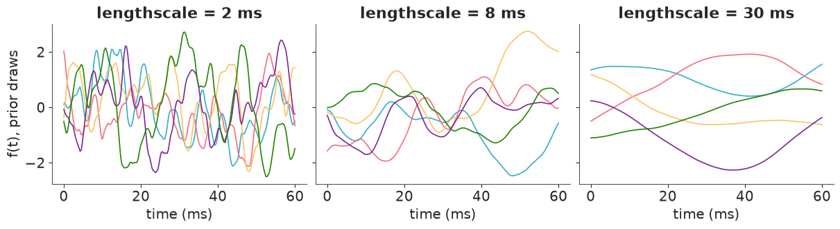
With $\ell = 2$ ms the functions wiggle faster than the accelerometer samples - such a GP could chase every reading. With $\ell = 30$ ms (half the experiment) they are nearly straight lines and could never produce the plunge-and-rebound. The truth is in between, and the data cannot tell us much outside that range:
- lengthscales far below the spacing of the inputs are indistinguishable from noise;
- lengthscales far above the span of the inputs are indistinguishable from a constant or a line.
A flat or very wide prior on $\ell$ therefore leaves the posterior free to drift into regions where the likelihood is flat - a classic source of bad GP fits.
3 · Priors that respect the data scale
For $\ell$ we want little mass below ~3 ms (the median gap between reading times is 0.4 ms, so this is already several samples) and little above ~25 ms (the whole record is 55 ms). An inverse-gamma is the usual choice because its left tail falls to zero very fast - it firmly rules out tiny lengthscales - while the right tail is heavy and forgiving.
Rather than fiddle with alpha and beta, ask PreliZ for the maximum-entropy
inverse-gamma with 90% of its mass between 3 and 25:
ell_prior = pz.maxent(pz.InverseGamma(), lower=3, upper=25, mass=0.9, plot=False)
ELL_ALPHA, ELL_BETA = float(ell_prior.alpha), float(ell_prior.beta)

print(ell_prior)
print("P(ell < 3) = %.3f,  P(ell > 25) = %.3f" % (ell_prior.cdf(3), 1 - ell_prior.cdf(25)))

fig, ax = plt.subplots(figsize=(7, 3))
grid = np.linspace(0.01, 60, 400)
ax.plot(grid, ell_prior.pdf(grid))
ax.axvspan(3, 25, color="k", alpha=0.08, label="90% of the mass")
ax.set(xlabel="lengthscale (ms)", ylabel="prior density", yticks=[])
ax.legend();
InverseGamma(alpha=3.35, beta=32.8)
P(ell < 3) = 0.002,  P(ell > 25) = 0.098
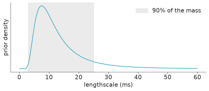
Note how the 10% that is left over is split: almost nothing below 3 ms, nearly all of it in the right tail. That asymmetry is the point of the inverse-gamma.
For the amplitude, y is in standard-deviation units, so the curve's swings are of order 1:
HalfNormal(1.5) allows up to ~3 while preferring less. Same for the noise, HalfNormal(1).
Prior predictive check. Do not take those words on trust - draw hyperparameters from the priors, then a function for each, and look.
with pm.Model():
    ell_ = pm.InverseGamma("ell", alpha=ELL_ALPHA, beta=ELL_BETA)
    eta_ = pm.HalfNormal("eta", 1.5)
    ell_draws, eta_draws = pm.draw([ell_, eta_], draws=12, random_seed=RANDOM_SEED)

fig, ax = plt.subplots(figsize=(8, 4))
for ell_i, eta_i in zip(ell_draws, eta_draws):
    K = (eta_i**2 * pm.gp.cov.Matern52(1, ls=ell_i))(t_grid[:, None]).eval()
    f_draw = rng.multivariate_normal(np.zeros(len(t_grid)), K + 1e-8 * np.eye(len(t_grid)))
    ax.plot(t_grid, f_draw * ACCEL_SD, lw=1, alpha=0.8)
ax.scatter(t, y * ACCEL_SD, s=8, color="k", alpha=0.4, zorder=3)
ax.set(xlabel="time (ms)", ylabel="acceleration (g)", title="Functions drawn from the prior (data in grey for scale)");
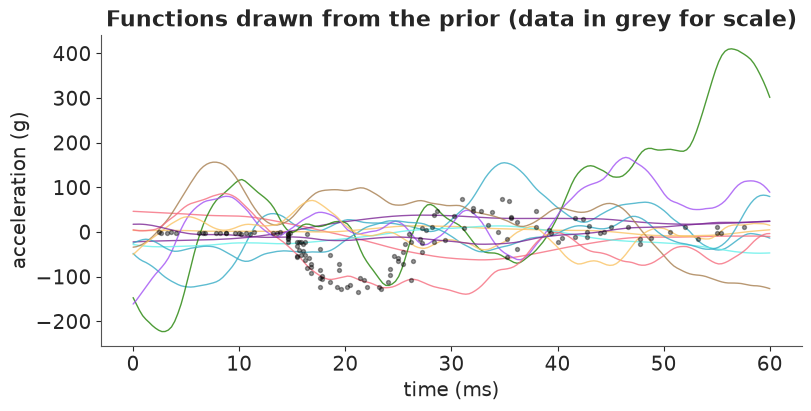
Most prior functions swing by tens to a couple of hundred g - the vertical scale of the data - with the occasional larger one from the tail of the amplitude prior, and they change on timescales from a few to a few tens of milliseconds. None of them looks like the data - they are not supposed to - but the data's shape is clearly within reach. That is what a weakly informative GP prior looks like.
4 · The exact GP: pm.gp.Marginal
With a Normal likelihood, $y_i = f(t_i) + \varepsilon_i$, $\varepsilon_i \sim \text{Normal}(0, \sigma)$, the function values can be integrated out analytically:
$$y \sim \text{MvNormal}\big(0,\ K + \sigma^2 I\big).$$
pm.gp.Marginal implements exactly this. NUTS only has to explore the three
hyperparameters $(\ell, \eta, \sigma)$; the 133 function values never appear as parameters.
with pm.Model() as exact_model:
    ell = pm.InverseGamma("ell", alpha=ELL_ALPHA, beta=ELL_BETA)
    eta = pm.HalfNormal("eta", 1.5)
    sigma = pm.HalfNormal("sigma", 1)

    cov = eta**2 * pm.gp.cov.Matern52(1, ls=ell)
    gp_exact = pm.gp.Marginal(cov_func=cov)
    gp_exact.marginal_likelihood("y", X=t[:, None], y=y, sigma=sigma)

    start = time.time()
    exact_idata = pm.sample(random_seed=RANDOM_SEED)
    exact_seconds = time.time() - start

print("divergences:", int(exact_idata.sample_stats["diverging"].sum()))
az.summary(exact_idata, ci_kind="hdi", ci_prob=0.94, round_to=2)
divergences: 0
| mean | sd | hdi94_lb | hdi94_ub | ess_bulk | ess_tail | r_hat | mcse_mean | mcse_sd | |
|---|---|---|---|---|---|---|---|---|---|
| ell | 7.62 | 1.74 | 4.48 | 10.71 | 1498.18 | 1609.46 | 1.0 | 0.05 | 0.03 |
| eta | 1.21 | 0.40 | 0.60 | 1.91 | 1494.06 | 1669.48 | 1.0 | 0.01 | 0.01 |
| sigma | 0.47 | 0.03 | 0.42 | 0.53 | 3096.31 | 2842.19 | 1.0 | 0.00 | 0.00 |
Clean diagnostics. The lengthscale is around 7 ms, comfortably inside the prior's bulk, and
the noise is just under half a standard deviation of y.
Predicting: gp.conditional
The function was integrated out, so to see it we must bring it back. Conditional on the
hyperparameters and the data, $f$ at new inputs is again multivariate Normal, with the
textbook GP mean and covariance. gp.conditional adds that distribution to the model, and
pm.sample_posterior_predictive draws from it once per posterior draw of the
hyperparameters. pred_noise=True gives new readings instead of the latent curve.
with exact_model:
    gp_exact.conditional("f_new", Xnew=t_grid[:, None])
    gp_exact.conditional("y_new", Xnew=t_grid[:, None], pred_noise=True)
    exact_pred = pm.sample_posterior_predictive(
        exact_idata, var_names=["f_new", "y_new"], random_seed=RANDOM_SEED
    )
def band(da, prob=0.94):
    """Mean and central interval over (chain, draw), rescaled to g."""
    lo, hi = da.quantile([(1 - prob) / 2, (1 + prob) / 2], dim=("chain", "draw")).to_numpy()
    return da.mean(("chain", "draw")).to_numpy() * ACCEL_SD, lo * ACCEL_SD, hi * ACCEL_SD


def plot_fit(f_da, y_da, ax, color="C0", title=None):
    """Latent curve (dark band) and predictive interval for new readings (light band)."""
    f_mean, f_lo, f_hi = band(f_da)
    _, y_lo, y_hi = band(y_da)
    ax.fill_between(t_grid, y_lo, y_hi, color=color, alpha=0.15, label="94% predictive (new readings)")
    ax.fill_between(t_grid, f_lo, f_hi, color=color, alpha=0.45, label="94% band for f")
    ax.plot(t_grid, f_mean, color=color)
    ax.scatter(t, y * ACCEL_SD, s=10, color="k", zorder=3)
    ax.set(xlabel="time (ms)", ylabel="acceleration (g)", title=title)


fig, ax = plt.subplots(figsize=(8, 4))
plot_fit(exact_pred.posterior_predictive["f_new"], exact_pred.posterior_predictive["y_new"], ax,
         title="Exact GP, constant noise")
ax.legend(loc="lower right");
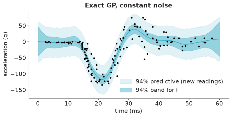
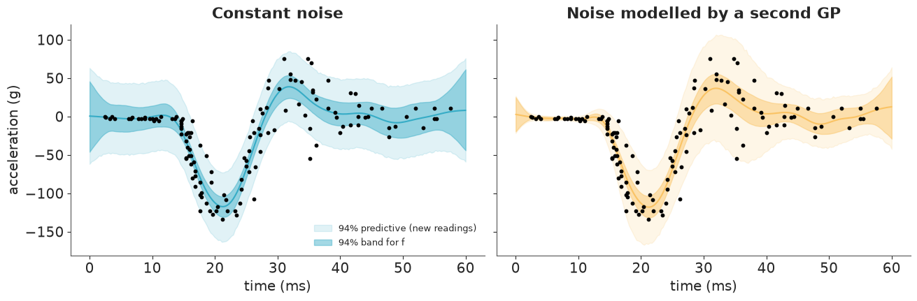
The curve is convincing. The light band is not: it has the same width everywhere, so in the first 13 ms it is an order of magnitude wider than the scatter of the readings, and around the rebound it looks too narrow. One $\sigma$ has to serve the whole record. We will fix that in section 7 - but the fix needs a latent GP inside a bigger model, and that is where exact GPs become painful.
5 · Why exact GPs do not scale
Every evaluation of that MvNormal density needs the Cholesky factor of the $n \times n$ matrix $K + \sigma^2 I$. That costs $O(n^3)$ time and $O(n^2)$ memory, and NUTS needs it (and its gradient) at every leapfrog step - thousands of times per fit. Time the factorisation alone:
sizes = np.array([250, 500, 1000, 2000, 4000])
chol_seconds = []
for n in sizes:
    x = np.sort(rng.uniform(0, 60, n))[:, None]
    # Matern-5/2 kernel written out in NumPy: evaluating PyMC's symbolic kernel here would
    # compile a function that keeps ~2 GB of intermediates alive for the rest of the notebook
    r = np.sqrt(5.0) * np.abs(x - x.T) / 7.0
    K = (1.0 + r + r**2 / 3.0) * np.exp(-r) + 0.2 * np.eye(n)
    del r
    best = np.inf
    for _ in range(3):  # best of three, to reduce timing noise
        start = time.perf_counter()
        np.linalg.cholesky(K)
        best = min(best, time.perf_counter() - start)
    chol_seconds.append(best)
del K

fig, ax = plt.subplots(figsize=(6, 3.5))
ax.loglog(sizes, chol_seconds, "o-", label="measured")
ax.loglog(sizes, chol_seconds[-1] * (sizes / sizes[-1]) ** 3.0, "k--", lw=1, label="$n^3$ reference")
ax.set(xlabel="number of observations n", ylabel="seconds per Cholesky")
ax.set_xticks(sizes, labels=[str(n) for n in sizes])
ax.minorticks_off()
ax.legend();

print(pd.Series(chol_seconds, index=sizes, name="seconds").round(4).to_string())
250     0.0001
500     0.0004
1000    0.0025
2000    0.0168
4000    0.1560
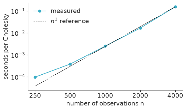
For large $n$ the measured line runs parallel to the $n^3$ reference: doubling the data
multiplies the cost by about eight. 133 points are nothing, a few thousand is a coffee
break per fit, tens of thousands is not feasible. And if the likelihood is not Normal, or
the GP is one component of a bigger model (as it will be in section 7 and in challenge
C08), $f$ cannot be integrated out at all: you need pm.gp.Latent, which adds $n$ strongly
correlated parameters on top of the $O(n^3)$ cost.
6 · The Hilbert-space approximation (HSGP)
The idea (Solin & Särkkä 2020; Riutort-Mayol et al. 2022): on an interval $[-L, L]$, any stationary GP can be approximated by a linear model with $m$ fixed basis functions,
$$f(t) \approx \sum_{j=1}^{m} \sqrt{S_\theta\big(\sqrt{\lambda_j}\big)}\;\phi_j(t)\;\beta_j, \qquad \beta_j \sim \text{Normal}(0, 1),$$
where $\phi_j(t) = \sqrt{1/L}\,\sin\!\big(\sqrt{\lambda_j}\,(t + L)\big)$ are sine waves of increasing frequency $\sqrt{\lambda_j} = j\pi / 2L$, and $S_\theta$ is the kernel's power spectral density - how much variance the kernel puts at each frequency.
- The basis $\phi_j$ does not depend on the hyperparameters: it is computed once.
- $\ell$ and $\eta$ only enter through the weights $\sqrt{S_\theta}$: a long lengthscale switches the high-frequency sines off, a short one turns them on.
- Cost per gradient: $O(nm)$ instead of $O(n^3)$. It is just a regression.
Look at both ingredients:
from pymc.gp.hsgp_approx import calc_eigenvalues, calc_eigenvectors

t_center = (t.max() + t.min()) / 2
half_range = (t.max() - t.min()) / 2
tc_grid = np.linspace(-half_range, half_range, 300)[:, None]  # HSGP works on centred inputs


def hsgp_pieces(m, c, ell):
    """Basis functions on tc_grid and sqrt-PSD weights of a unit-amplitude Matern52."""
    L = np.array([c * half_range])
    eigvals = calc_eigenvalues(L, [m])
    phi = calc_eigenvectors(tc_grid, L, eigvals, [m])
    phi = phi.eval() if hasattr(phi, "eval") else np.asarray(phi)
    psd = pm.gp.cov.Matern52(1, ls=ell).power_spectral_density(np.sqrt(eigvals)).eval().ravel()
    return phi, psd


phi, _ = hsgp_pieces(m=40, c=1.5, ell=1.0)
fig, axes = plt.subplots(1, 2, figsize=(12, 3.5))
for j in [0, 1, 2, 7]:
    axes[0].plot(tc_grid + t_center, phi[:, j], label=f"$\\phi_{{{j + 1}}}$")
axes[0].set(xlabel="time (ms)", title="Basis functions (fixed)")
axes[0].legend(ncol=4, fontsize=9)
for ell_i in [3, 8, 25]:
    _, psd = hsgp_pieces(m=40, c=1.5, ell=ell_i)
    axes[1].plot(np.arange(1, 41), np.sqrt(psd), "o-", ms=3, label=f"$\\ell$ = {ell_i} ms")
axes[1].set(xlabel="basis function j", ylabel="weight $\\sqrt{S(\\sqrt{\\lambda_j})}$",
            title="Weights (depend on the lengthscale)")
axes[1].legend();
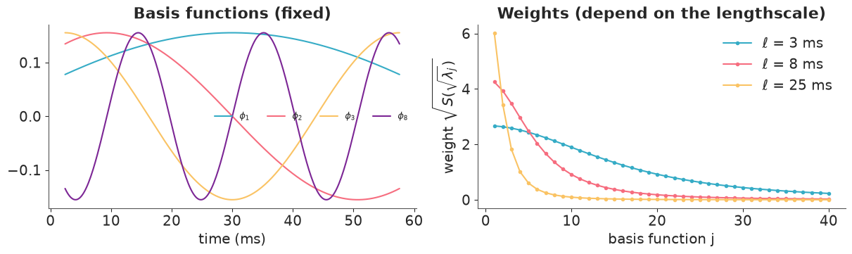
With $\ell = 25$ ms only the first handful of sines matter; with $\ell = 3$ ms the weights are still far from zero at $j = 40$, so truncating there would throw away real wiggliness.
Choosing m and c
Two knobs, two failure modes:
csets the boundary $L = c \times$ (half-range of the inputs). The sines are forced to zero at $\pm L$, so $f$ is pinned there. For long lengthscales that pinning is felt far inside the domain: you need a largerc. If you will predict outside the training range, that range must be inside $[-L, L]$ too.mis the number of sines. Short lengthscales need high frequencies: largerm. And a largercstretches the sines, so it also demands a largerm.
PyMC ships the heuristic from Riutort-Mayol et al. Feed it the range of inputs and the range of lengthscales your prior considers plausible:
m_rec, c_rec = pm.gp.hsgp_approx.approx_hsgp_hyperparams(
    x_range=[t.min(), t.max()], lengthscale_range=[3, 25], cov_func="matern52"
)
print(f"recommended: m = {m_rec}, c = {c_rec:.2f}")
recommended: m = 90, c = 3.71
Trust, but verify. The approximation implies a covariance matrix $\Phi\,\text{diag}(S)\,\Phi^\top$ that we can compare with the true kernel directly, for the recommended setting and for a stingy one. Top row: the covariance between the centre of the record and every other time. Bottom row: the prior variance of $f(t)$ itself, which should be 1 everywhere.
fig, axes = plt.subplots(2, 3, figsize=(12, 5.5), sharex=True, sharey="row")
mid = len(tc_grid) // 2
settings = [((m_rec, c_rec), "C0-"), ((15, 1.2), "C3--")]
for col, ell_i in enumerate([3, 8, 25]):
    K_true = pm.gp.cov.Matern52(1, ls=ell_i)(tc_grid).eval()
    axes[0, col].plot(tc_grid + t_center, K_true[mid], "k", lw=4, alpha=0.25, label="exact kernel")
    axes[1, col].axhline(1, color="k", lw=4, alpha=0.25)
    for (m_i, c_i), style in settings:
        phi, psd = hsgp_pieces(m_i, c_i, ell_i)
        K_approx = phi @ np.diag(psd) @ phi.T
        axes[0, col].plot(tc_grid + t_center, K_approx[mid], style, lw=1.3, label=f"m={m_i}, c={c_i:.1f}")
        axes[1, col].plot(tc_grid + t_center, np.diag(K_approx), style, lw=1.3)
        print(f"ell = {ell_i:>2} ms, m = {m_i:>2}, c = {c_i:.1f}: "
              f"largest error anywhere in the covariance matrix = {np.abs(K_approx - K_true).max():.3f}")
    axes[0, col].set_title(f"$\\ell$ = {ell_i} ms")
    axes[1, col].set(xlabel="time (ms)", ylim=(0, 1.2))
axes[0, 0].set_ylabel("cov(f(t), f(30 ms))")
axes[1, 0].set_ylabel("var(f(t))")
axes[0, 2].legend(fontsize=9, loc="lower center");
ell =  3 ms, m = 90, c = 3.7: largest error anywhere in the covariance matrix = 0.009
ell =  3 ms, m = 15, c = 1.2: largest error anywhere in the covariance matrix = 0.112
ell =  8 ms, m = 90, c = 3.7: largest error anywhere in the covariance matrix = 0.000
ell =  8 ms, m = 15, c = 1.2: largest error anywhere in the covariance matrix = 0.335
ell = 25 ms, m = 90, c = 3.7: largest error anywhere in the covariance matrix = 0.000
ell = 25 ms, m = 15, c = 1.2: largest error anywhere in the covariance matrix = 0.862
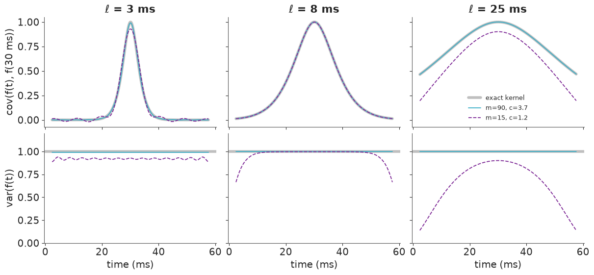
The recommended setting reproduces the kernel at all three lengthscales: the largest error
anywhere in the covariance matrix is 0.009, at $\ell = 3$ ms. The stingy one (m=15,
c=1.2) fails in two different ways:
- Too few sines (
m): at $\ell = 3$ ms it lacks the high frequencies to form a narrow peak. The peak comes out too low, with ripples either side, and the prior variance sits below 1. - Boundary too close (
c): the variance is pinched towards zero at the edges of the record. At $\ell = 8$ ms that only hurts the first and last few milliseconds; at $\ell = 25$ ms it ruins the whole domain (largest error 0.86 - the approximation is nothing like the kernel we asked for). A model fitted with it would be confidently flat near the edges.
Fitting it
gp.prior("f", X) builds the regression above and returns $f$ at the rows of X. Three
details matter:
Xis apm.Datacontainer.HSGPrecords the centre and the boundaryLfrom the training inputs when the model is built, so that swapping in new inputs later withpm.set_dataevaluates the same basis at new locations. (If you want the basis and the weights themselves - for instance to share one basis between several GPs -gp.prior_linearized(X)returns them and you writephi @ (beta * sqrt_psd)yourself.)- The likelihood gets
shape=f.shapeso that it resizes with the data. - Freeze the data while sampling. A
pm.Datacontainer may change at any time, so the compiled model recomputes the whole sine basis at every gradient evaluation - which throws away the main selling point of HSGP.freeze_dims_and_data(model)returns a copy in which the data are constants, so the basis is computed once. Sample from the frozen copy; keep the original forpm.set_data. We time both below.
def build_hsgp(parametrization):
    with pm.Model() as model:
        X = pm.Data("X", t[:, None])
        ell = pm.InverseGamma("ell", alpha=ELL_ALPHA, beta=ELL_BETA)
        eta = pm.HalfNormal("eta", 1.5)
        sigma = pm.HalfNormal("sigma", 1)

        cov = eta**2 * pm.gp.cov.Matern52(1, ls=ell)
        gp = pm.gp.HSGP(m=[m_rec], c=c_rec, parametrization=parametrization, cov_func=cov)
        f = gp.prior("f", X=X)
        pm.Normal("y", f, sigma, observed=y, shape=f.shape)
    return model


hsgp_nc_model = build_hsgp("noncentered")

start = time.time()
with hsgp_nc_model:  # pm.Data left as it is: the basis is rebuilt at every gradient
    pm.sample(random_seed=RANDOM_SEED, progressbar=False)
unfrozen_seconds = time.time() - start

start = time.time()
with freeze_dims_and_data(hsgp_nc_model):
    hsgp_nc_idata = pm.sample(random_seed=RANDOM_SEED)
frozen_seconds = time.time() - start

print(f"sampling wall time: {unfrozen_seconds:.0f}s with live pm.Data, {frozen_seconds:.0f}s frozen")

print("divergences:", int(hsgp_nc_idata.sample_stats["diverging"].sum()))
az.summary(hsgp_nc_idata, var_names=["ell", "eta", "sigma"], ci_kind="hdi", ci_prob=0.94, round_to=2)
sampling wall time: 6s with live pm.Data, 1s frozen
divergences: 165
| mean | sd | hdi94_lb | hdi94_ub | ess_bulk | ess_tail | r_hat | mcse_mean | mcse_sd | |
|---|---|---|---|---|---|---|---|---|---|
| ell | 7.45 | 1.57 | 4.87 | 10.47 | 206.51 | 56.67 | 1.03 | 0.12 | 0.08 |
| eta | 1.19 | 0.40 | 0.55 | 1.92 | 105.77 | 42.09 | 1.05 | 0.05 | 0.07 |
| sigma | 0.47 | 0.03 | 0.42 | 0.53 | 1684.02 | 1762.44 | 1.01 | 0.00 | 0.00 |
First the timing: freezing the data made sampling several times faster even on this tiny problem (both numbers include a few seconds of compilation), and the gap grows with $n$ and $m$. From here on we always sample from the frozen copy.
The estimates agree with the exact GP, but look at the divergence count, the r_hat and the
ESS of ell and eta, an order of magnitude below that of sigma. You have seen this in
E02: it is the centred/non-centred story with the roles reversed.
By default HSGP is non-centred: $\beta_j \sim \text{Normal}(0, 1)$ and $f = \Phi\,(\sqrt{S_\theta} \odot \beta)$. That is the right choice when the data say little about $f$. Here the data pin the curve down tightly, so the products $\sqrt{S_\theta(j)}\,\beta_j$ are well determined - and every change in $\ell$ or $\eta$ must be compensated by all the $\beta_j$ at once. That is a curved, funnel-like posterior. The centred form samples the products directly, $\beta_j \sim \text{Normal}(0, \sqrt{S_\theta(j)})$:
hsgp_model = build_hsgp("centered")
with freeze_dims_and_data(hsgp_model):
    hsgp_idata = pm.sample(draws=2000, random_seed=RANDOM_SEED)  # 2000 draws: see below

print("divergences:", int(hsgp_idata.sample_stats["diverging"].sum()))
az.summary(hsgp_idata, var_names=["ell", "eta", "sigma"], ci_kind="hdi", ci_prob=0.94, round_to=2)
divergences: 0
| mean | sd | hdi94_lb | hdi94_ub | ess_bulk | ess_tail | r_hat | mcse_mean | mcse_sd | |
|---|---|---|---|---|---|---|---|---|---|
| ell | 7.51 | 1.69 | 4.55 | 10.70 | 559.72 | 1077.55 | 1.01 | 0.07 | 0.04 |
| eta | 1.18 | 0.38 | 0.61 | 1.90 | 1105.33 | 2050.90 | 1.00 | 0.01 | 0.01 |
| sigma | 0.47 | 0.03 | 0.41 | 0.53 | 11209.49 | 5611.28 | 1.00 | 0.00 | 0.00 |
The divergences are gone and r_hat is back to 1.00-1.01. That is what matters most:
divergences mean the sampler is missing part of the posterior, which biases everything
downstream.
The centred form is not free, though: the ESS of ell is still well under a tenth of the
number of draws. Of the 90 coefficients only the low-frequency ones are pinned down by the
data; the high-frequency rest are governed by their prior, and for those the centred form
is the funnel (their prior scale $\sqrt{S_\theta(j)}$ moves with $\ell$). Neither
parametrisation is right for all 90 at once. Slow-but-unbiased mixing is the better problem
to have - it is cured by running longer, which is why this fit uses 2000 draws per chain.
Predicting with pm.set_data
No conditional needed: $f$ is a deterministic function of X and the coefficients, so we
swap X and ask for f and y at the new inputs.
with hsgp_model:
    pm.compute_log_likelihood(hsgp_idata)  # for LOO later; do this while X is still the training data
    pm.sample_posterior_predictive(hsgp_idata, extend_inferencedata=True, random_seed=RANDOM_SEED)
    pm.set_data({"X": t_grid[:, None]})
    hsgp_pred = pm.sample_posterior_predictive(
        hsgp_idata, var_names=["f", "y"], predictions=True, random_seed=RANDOM_SEED
    )
Does it agree with the exact GP?
fig, ax = plt.subplots(figsize=(8, 4))
for da, color, label in [(exact_pred.posterior_predictive["f_new"], "C0", "exact"),
                         (hsgp_pred.predictions["f"], "C1", f"HSGP (m={m_rec})")]:
    mean, lo, hi = band(da)
    ax.plot(t_grid, mean, color=color, label=label)
    ax.plot(t_grid, lo, color=color, lw=0.8, ls="--")
    ax.plot(t_grid, hi, color=color, lw=0.8, ls="--")
ax.scatter(t, y * ACCEL_SD, s=8, color="k", alpha=0.4)
ax.set(xlabel="time (ms)", ylabel="acceleration (g)", title="Posterior mean and 94% band of f")
ax.legend();
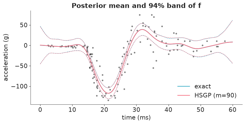
f_gap = np.abs(band(exact_pred.posterior_predictive["f_new"])[0] - band(hsgp_pred.predictions["f"])[0]).max()
print(f"largest gap between the two posterior means of f: {f_gap:.2f} g")
print(f"sampling wall time, 1000 draws: exact {exact_seconds:.0f}s, HSGP {frozen_seconds:.0f}s (frozen)")

rows = {}
for name, idata in [("exact", exact_idata), ("HSGP", hsgp_idata)]:
    post = az.extract(idata, var_names=["ell", "eta", "sigma"])
    rows[name] = {v: f"{float(post[v].mean()):.2f} ± {float(post[v].std()):.2f}" for v in ["ell", "eta", "sigma"]}
pd.DataFrame(rows).T.rename_axis("posterior mean ± sd")
largest gap between the two posterior means of f: 0.42 g
sampling wall time, 1000 draws: exact 5s, HSGP 1s (frozen)
| ell | eta | sigma | |
|---|---|---|---|
| posterior mean ± sd | |||
| exact | 7.62 ± 1.74 | 1.21 ± 0.40 | 0.47 ± 0.03 |
| HSGP | 7.51 ± 1.69 | 1.18 ± 0.38 | 0.47 ± 0.03 |
The curves and bands are on top of each other and the hyperparameters match to within Monte Carlo error. On 133 points speed is not the argument - both models fit in a few seconds, most of it compilation, and your timings will differ. The pay-off is elsewhere: HSGP's cost grows linearly in $n$ instead of cubically, and because $f$ is now an ordinary deterministic node, we can use GPs as building blocks - which is what we do next.
When not to use HSGP: lengthscales that are tiny relative to the domain (the required m
explodes), more than 2-3 input dimensions (m is per dimension and multiplies), or
non-stationary kernels (no spectral density).
7 · The pay-off: a GP for the noise, too
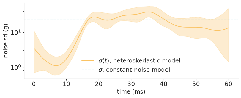
The constant-noise band in section 4 was wrong. Let the noise level itself be a smooth function of time, modelled on the log scale so that it stays positive:
$$ \begin{aligned} y_i &\sim \text{Normal}\big(f(t_i),\ \sigma(t_i)\big) \\ f &\sim \text{GP}(0, k_f) \\ \log \sigma(t) &= s_0 + g(t), \qquad g \sim \text{GP}(0, k_g) \end{aligned} $$
With exact GPs this is unpleasant ($\sigma(t)$ sits inside the covariance matrix, and $g$
must be a 133-dimensional Latent GP). With HSGP it is ten more lines.
Priors: $s_0 \sim \text{Normal}(-1, 1)$ puts the typical noise around $e^{-1} \approx 0.4$
sd units with a factor of $e$ either way. eta_g ~ HalfNormal(1.5) lets the noise vary over
time by a factor of up to $e^{\pm 3}$ - wide, because the plot suggests a change of more
than tenfold. Same lengthscale prior as $f$.
Parametrisation, following the reasoning above: $f$ is strongly informed by the data →
centred; $g$ is only weakly informed (a variance is much harder to learn than a mean)
→ non-centred. Two GPs multiply the awkward geometry, so we also raise target_accept
and, as before, take 2000 draws per chain.
with pm.Model() as hetero_model:
    X = pm.Data("X", t[:, None])

    ell = pm.InverseGamma("ell", alpha=ELL_ALPHA, beta=ELL_BETA)
    eta = pm.HalfNormal("eta", 1.5)
    gp_f = pm.gp.HSGP(m=[m_rec], c=c_rec, parametrization="centered",
                      cov_func=eta**2 * pm.gp.cov.Matern52(1, ls=ell))
    f = gp_f.prior("f", X=X)

    ell_g = pm.InverseGamma("ell_g", alpha=ELL_ALPHA, beta=ELL_BETA)
    eta_g = pm.HalfNormal("eta_g", 1.5)
    s0 = pm.Normal("s0", -1, 1)
    gp_g = pm.gp.HSGP(m=[m_rec], c=c_rec, parametrization="noncentered",
                      cov_func=eta_g**2 * pm.gp.cov.Matern52(1, ls=ell_g))
    g = gp_g.prior("g", X=X)
    sigma_t = pm.Deterministic("sigma_t", pm.math.exp(s0 + g))

    pm.Normal("y", f, sigma_t, observed=y, shape=f.shape)


with freeze_dims_and_data(hetero_model):
    hetero_idata = pm.sample(draws=2000, target_accept=0.95, random_seed=RANDOM_SEED)

print("divergences:", int(hetero_idata.sample_stats["diverging"].sum()))
az.summary(hetero_idata, var_names=["ell", "eta", "ell_g", "eta_g", "s0"],
           ci_kind="hdi", ci_prob=0.94, round_to=2)
divergences: 0
| mean | sd | hdi94_lb | hdi94_ub | ess_bulk | ess_tail | r_hat | mcse_mean | mcse_sd | |
|---|---|---|---|---|---|---|---|---|---|
| ell | 7.57 | 1.60 | 4.69 | 10.56 | 633.09 | 1039.29 | 1.01 | 0.06 | 0.03 |
| eta | 1.15 | 0.38 | 0.59 | 1.84 | 1450.06 | 2192.69 | 1.00 | 0.01 | 0.01 |
| ell_g | 8.95 | 2.58 | 4.66 | 13.68 | 6139.42 | 6028.15 | 1.00 | 0.03 | 0.04 |
| eta_g | 1.46 | 0.48 | 0.73 | 2.33 | 6095.39 | 5880.70 | 1.00 | 0.01 | 0.01 |
| s0 | -1.42 | 0.61 | -2.51 | -0.19 | 7713.84 | 5174.31 | 1.00 | 0.01 | 0.01 |
az.plot_rank(hetero_idata, var_names=["ell", "eta", "ell_g", "eta_g", "s0"]);
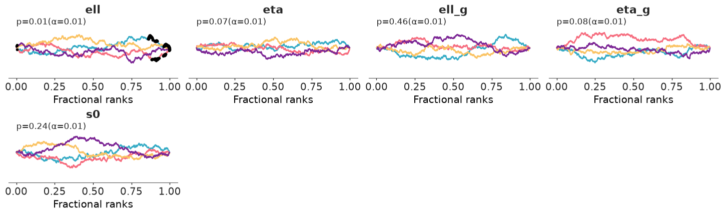
No divergences and r_hat at most 1.01. The weakest parameter is ell again: it has the
lowest ESS, and its rank plot touches the edge of the 99% envelope at the high end (marked
in black) - the slow mixing of the centred form that we met above. For the curve and the
bands, which is what we use below, that is good enough; if $\ell$ itself were the quantity
of interest we would run longer.
with hetero_model:
    pm.compute_log_likelihood(hetero_idata)
    pm.sample_posterior_predictive(hetero_idata, extend_inferencedata=True, random_seed=RANDOM_SEED)
    pm.set_data({"X": t_grid[:, None]})
    hetero_pred = pm.sample_posterior_predictive(
        hetero_idata, var_names=["f", "y", "sigma_t"], predictions=True, random_seed=RANDOM_SEED
    )
Posterior predictive check: whose bands are right?
fig, axes = plt.subplots(1, 2, figsize=(13, 4.2), sharey=True)
plot_fit(hsgp_pred.predictions["f"], hsgp_pred.predictions["y"], axes[0], color="C0",
         title="Constant noise")
plot_fit(hetero_pred.predictions["f"], hetero_pred.predictions["y"], axes[1], color="C2",
         title="Noise modelled by a second GP")
axes[1].set_ylabel("")
axes[0].legend(loc="lower right", fontsize=9);
fig, ax = plt.subplots(figsize=(8, 3.2))
s_mean, s_lo, s_hi = band(hetero_pred.predictions["sigma_t"])
ax.fill_between(t_grid, s_lo, s_hi, color="C2", alpha=0.3)
ax.plot(t_grid, s_mean, color="C2", label="$\\sigma(t)$, heteroskedastic model")
ax.axhline(float(hsgp_idata.posterior["sigma"].mean()) * ACCEL_SD, color="C0", ls="--",
           label="$\\sigma$, constant-noise model")
ax.set(xlabel="time (ms)", ylabel="noise sd (g)", yscale="log")
ax.legend();
A picture is persuasive; a number is checkable. How many readings fall inside each model's own 90% predictive interval, by phase of the crash? A calibrated model scores about 90% in every phase, not just on average.
phase = pd.cut(t, [0, 13, 30, 40, 60],
               labels=["before impact (<13 ms)", "impact (13-30 ms)", "rebound (30-40 ms)", "tail (>40 ms)"])


def coverage_by_phase(idata, prob=0.9):
    y_rep = idata.posterior_predictive["y"]
    lo, hi = y_rep.quantile([(1 - prob) / 2, (1 + prob) / 2], dim=("chain", "draw")).to_numpy()
    inside = (y >= lo) & (y <= hi)
    width = (hi - lo) * ACCEL_SD
    out = pd.DataFrame({"inside": inside, "width": width}).groupby(phase, observed=True).agg(
        n=("inside", "size"), coverage=("inside", "mean"), mean_width_g=("width", "mean"))
    return out.round(2)


pd.concat({"constant noise": coverage_by_phase(hsgp_idata),
           "heteroskedastic": coverage_by_phase(hetero_idata)}, axis=1)
| constant noise | heteroskedastic | |||||
|---|---|---|---|---|---|---|
| n | coverage | mean_width_g | n | coverage | mean_width_g | |
| before impact (<13 ms) | 18 | 1.00 | 80.28 | 18 | 1.00 | 6.12 |
| impact (13-30 ms) | 72 | 0.90 | 77.38 | 72 | 0.94 | 75.36 |
| rebound (30-40 ms) | 22 | 0.82 | 78.69 | 22 | 0.95 | 119.17 |
| tail (>40 ms) | 21 | 1.00 | 81.33 | 21 | 1.00 | 55.88 |
The constant-noise model has one width for everything: about 80 g. Before the impact that is an interval 80 g wide around readings that vary by a couple of g. It covers 100% of them, but over-coverage is a failure too: this model would not notice a sensor fault ten times larger than anything in the data. In the rebound, where the scatter is largest, the same 80 g is too narrow and coverage drops to 82%.
The heteroskedastic model's interval is 6 g wide before the impact, about 120 g in the rebound and 56 g in the tail, and it covers 94-100% of the readings in every phase. That is slightly conservative for a nominal 90% - with about 20 readings in three of the phases, 100% instead of 90% is a matter of two readings - but it is never too narrow, and its widths follow the data.
LOO
Pointwise LOO needs a pointwise likelihood, which is another thing HSGP gives us. (The
Marginal model has a single 133-dimensional MvNormal "observation", so az.loo has
nothing to leave out.)
comparison = az.compare({"constant noise": hsgp_idata, "heteroskedastic": hetero_idata})
comparison
| rank | elpd_diff | dse | p_worse | diag_diff | diag_elpd | p | elpd | se | weight | |
|---|---|---|---|---|---|---|---|---|---|---|
| heteroskedastic | 0 | 0.0 | 0.0 | NaN | 5 k̂ > 0.70 | 22.5 | -40.0 | 14.0 | 1.0 | |
| constant noise | 1 | -50.0 | 10.0 | 1.0 | 12.0 | -90.0 | 10.0 | 0.0 |
az.plot_compare(comparison);
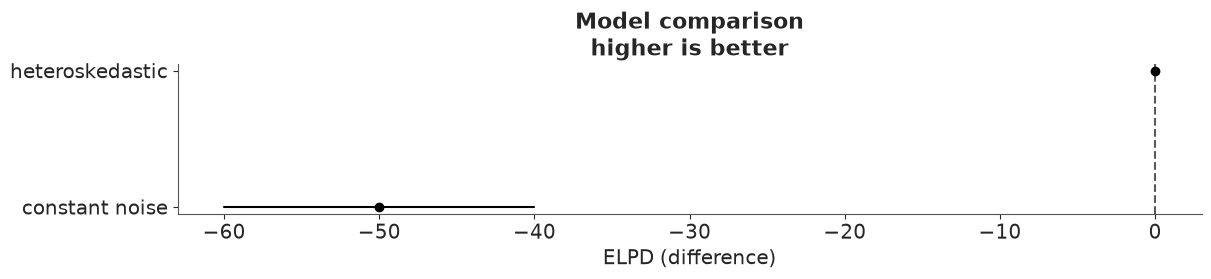
The heteroskedastic model wins by an elpd margin several times its standard error dse,
despite spending more effective parameters (p). If LOO warns about a few Pareto-$k$ values
above 0.7 for this model, that is expected: with a flexible noise process, a single reading
in a sparse stretch has a lot of influence on the local $\sigma(t)$, which is precisely the
situation where importance sampling struggles. The margin here is far too large for that to
change the verdict; when it is close, refit for the flagged points with az.reloo or use
az.loo_kfold.
What did we learn about the crash? The mean curve barely changed between models. What changed is the honesty of the uncertainty: a helmet engineer reading the first figure would conclude that readings are uncertain by tens of g at all times; the second says the rig is precise to a few g and the large scatter is a feature of the impact phase itself.
Try it yourself
- Replace
Matern52withExpQuadin the exact model and the centred HSGP. Compare the fits, then explain what goes wrong in the centred HSGP (hint: plot theExpQuadspectral density weights for large $j$ the way we did in section 6). - Halve and double
m(keepingc), and setc = 1.2(keepingm). Which posterior summaries move first - $\ell$, $\eta$, or the curve itself? - The readings look heavier-tailed than Normal during the rebound. Swap the likelihood of
the heteroskedastic model for a
StudentTwith an estimatednu. Does LOO prefer it, and do the Pareto-$k$ warnings go away?
Next: challenge C08, where HSGPs become components of a structural time-series model that has to forecast - something a stationary GP on its own turns out to be bad at.