A meta-analysis is the original privacy-preserving analysis. Each study keeps its patients
and publishes a handful of numbers - how many people in each arm, how many had the event -
and the analyst pools those numbers. The metadat database (the benchmark collection behind
the R package metafor) holds hundreds of such tables, and not one of them contains a person.
This notebook takes that seriously in both directions. First, the good news: for the models used here the published table loses nothing relative to the individual records, so there is no privacy-vs-accuracy trade-off at all. Then the cost of going further: when a database suppresses small counts or adds calibrated noise before release, the numbers it publishes are no longer the sufficient statistics, and an analysis that ignores that is not just noisier but wrong. Both mechanisms are modelled explicitly, and the loss of information is measured rather than guessed. Along the way, the usual visual tools of the trade are built by hand: forest, funnel, bubble, influence and cumulative plots.
import logging

import arviz as az
import matplotlib.pyplot as plt
import numpy as np
import pandas as pd
import pymc as pm
from scipy import stats

from pymc_challenges import data

RANDOM_SEED = 42
rng = np.random.default_rng(RANDOM_SEED)
az.style.use("arviz-variat")
logging.getLogger("pymc").setLevel(logging.WARNING)  # this notebook runs ~50 fits: no banner per fit
BLUE, ORANGE, AQUA, GREY = "#2a78d6", "#eb6834", "#1baf7a", "#8a8a86"
print(f"PyMC {pm.__version__}, ArviZ {az.__version__}")


def fit(model, **kw):
    """One place for the sampler settings; every fit reports its divergences."""
    with model:
        idata = pm.sample(target_accept=0.95, random_seed=RANDOM_SEED, progressbar=False, **kw)
    print(f"  {model.name or 'model'}: divergences = {int(idata.sample_stats['diverging'].sum())}")
    return idata


def stacked(da):
    return da.stack(sample=("chain", "draw")).transpose("sample", ...).to_numpy()
PyMC 6.3.2, ArviZ 1.3.0
1 · The database
Thirteen trials of the BCG vaccine against tuberculosis, published between 1948 and 1980 and run on four continents. Each is a 2 x 2 table plus two study-level facts: the year and the absolute latitude of the site (BCG is known to work better far from the equator, plausibly because exposure to environmental mycobacteria near the equator gives some natural immunity that the vaccine cannot add to). That is all we get: 13 rows.
data.describe("bcg")
bcg = data.load("bcg")
bcg["n_vacc"] = bcg.tpos + bcg.tneg
bcg["n_ctrl"] = bcg.cpos + bcg.cneg
bcg["rate_vacc"] = 1000 * bcg.tpos / bcg.n_vacc
bcg["rate_ctrl"] = 1000 * bcg.cpos / bcg.n_ctrl
bcg[["author", "year", "ablat", "alloc", "tpos", "n_vacc", "cpos", "n_ctrl", "rate_vacc", "rate_ctrl"]].round(1)
bcg: 13 trials as 2x2 tables (TB cases and non-cases in vaccinated / control arms), year, latitude, allocation.
  source: Colditz et al. (1994), BCG vaccine against tuberculosis; the `metafor`/`metadat` benchmark.
  url:    https://raw.githubusercontent.com/wviechtb/metadat/master/data-raw/dat.bcg.txt
| author | year | ablat | alloc | tpos | n_vacc | cpos | n_ctrl | rate_vacc | rate_ctrl | |
|---|---|---|---|---|---|---|---|---|---|---|
| 0 | Aronson | 1948 | 44 | random | 4 | 123 | 11 | 139 | 32.5 | 79.1 |
| 1 | Ferguson & Simes | 1949 | 55 | random | 6 | 306 | 29 | 303 | 19.6 | 95.7 |
| 2 | Rosenthal et al | 1960 | 42 | random | 3 | 231 | 11 | 220 | 13.0 | 50.0 |
| 3 | Hart & Sutherland | 1977 | 52 | random | 62 | 13598 | 248 | 12867 | 4.6 | 19.3 |
| 4 | Frimodt-Moller et al | 1973 | 13 | alternate | 33 | 5069 | 47 | 5808 | 6.5 | 8.1 |
| 5 | Stein & Aronson | 1953 | 44 | alternate | 180 | 1541 | 372 | 1451 | 116.8 | 256.4 |
| 6 | Vandiviere et al | 1973 | 19 | random | 8 | 2545 | 10 | 629 | 3.1 | 15.9 |
| 7 | TPT Madras | 1980 | 13 | random | 505 | 88391 | 499 | 88391 | 5.7 | 5.6 |
| 8 | Coetzee & Berjak | 1968 | 27 | random | 29 | 7499 | 45 | 7277 | 3.9 | 6.2 |
| 9 | Rosenthal et al | 1961 | 42 | systematic | 17 | 1716 | 65 | 1665 | 9.9 | 39.0 |
| 10 | Comstock et al | 1974 | 18 | systematic | 186 | 50634 | 141 | 27338 | 3.7 | 5.2 |
| 11 | Comstock & Webster | 1969 | 33 | systematic | 5 | 2498 | 3 | 2341 | 2.0 | 1.3 |
| 12 | Comstock et al | 1976 | 33 | systematic | 27 | 16913 | 29 | 17854 | 1.6 | 1.6 |
order = np.argsort(bcg.ablat.to_numpy())
fig, ax = plt.subplots(figsize=(9, 5.5))
for k, i in enumerate(order):
    r = bcg.iloc[i]
    ax.plot([r.rate_ctrl, r.rate_vacc], [k, k], color=GREY, lw=1 + np.log10(r.n_vacc + r.n_ctrl), zorder=1)
    ax.scatter(r.rate_ctrl, k, color=GREY, s=50, zorder=2)
    ax.scatter(r.rate_vacc, k, color=BLUE, s=50, zorder=3)
ax.set(yticks=range(len(bcg)), xlabel="tuberculosis cases per 1000 participants",
       title="Control (grey) vs vaccinated (blue) TB rate in each trial, ordered by latitude")
ax.set_yticklabels([f"{bcg.author[i]} ({bcg.year[i]}, {bcg.ablat[i]}°)" for i in order], fontsize=9)
ax.scatter([], [], color=GREY, label="control arm")
ax.scatter([], [], color=BLUE, label="BCG arm")
ax.legend(loc="lower right");
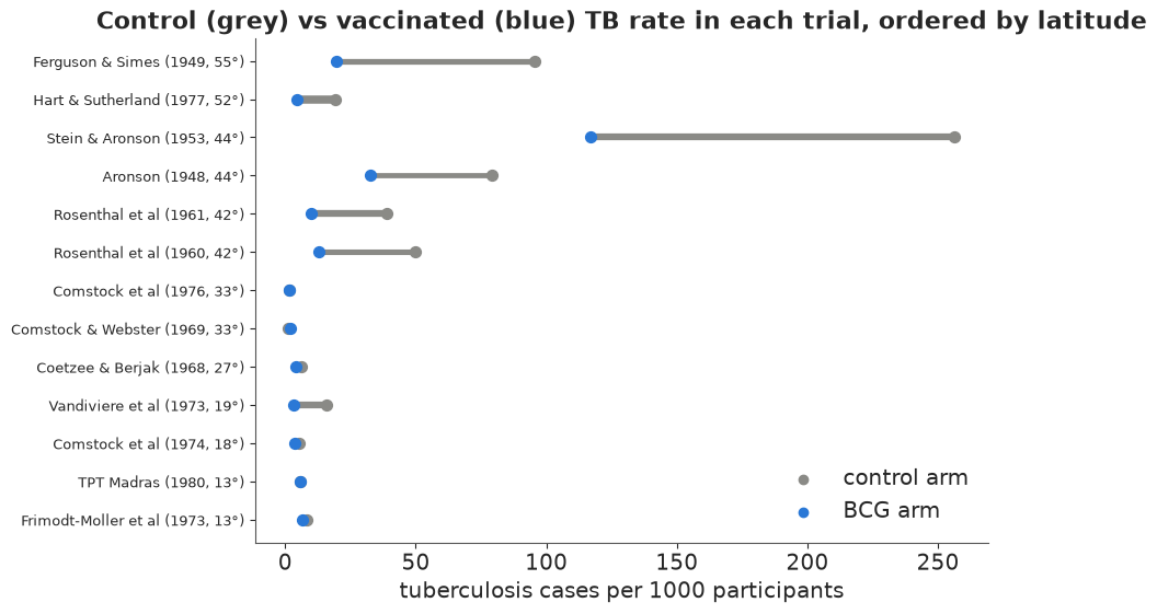
The picture already contains the whole story: the vaccine arm is to the left of the control arm in eleven of thirteen trials, the gap is larger at high latitude, and the trials differ enormously in size (the line thickness): from 260 to 177,000 participants.
Why the table loses nothing: sufficient statistics
Suppose we did have the individual records - one row per participant with arm and outcome. For a binary outcome and a model whose parameters are per-arm probabilities, the likelihood of those records is $\prod_i p_{\text{arm}(i)}^{y_i}(1-p_{\text{arm}(i)})^{1-y_i}$, which depends on the data only through the count of events per arm. The 2 x 2 table is a sufficient statistic: every posterior we could compute from the records we can compute from the table. Let us check that literally, on the first trial.
a, b, c, d = (bcg[col].to_numpy(float) for col in ["tpos", "tneg", "cpos", "cneg"])
i = 0
records = np.r_[np.ones(int(a[i])), np.zeros(int(b[i]))]  # the participant-level 0/1 outcomes, BCG arm

p_test = 0.03
lp_individual = pm.logp(pm.Bernoulli.dist(p=p_test), records).sum().eval()
lp_table = pm.logp(pm.Binomial.dist(n=a[i] + b[i], p=p_test), a[i]).eval()
log_binom_coef = stats.binom(a[i] + b[i], p_test).logpmf(a[i]) - (a[i] * np.log(p_test) + b[i] * np.log(1 - p_test))
print(f"individual records: {lp_individual:.3f}   table: {lp_table:.3f}   "
      f"difference = log binomial coefficient = {log_binom_coef:.3f} (a constant, so the posteriors agree)")
individual records: -17.651 table: -1.629 difference = log binomial coefficient = 16.021 (a constant, so the posteriors agree)
The two log-likelihoods differ by a constant that does not depend on $p$, so every posterior is identical. This is why the published table is, for this model, a lossless and anonymous summary: the privacy comes free. (The claim has limits: it needs the model to be a function of the arm-level counts only. Patient-level covariates, time-to-event outcomes or interactions between a treatment and an individual's characteristics need more than the table - that is where individual-participant-data meta-analysis, and its privacy problems, begin.)
2 · Two ways to pool: two-stage and one-stage
Two-stage. Reduce each trial to a log odds ratio $y_k$ and its standard error $s_k$, then treat $y_k \sim \text{Normal}(\theta_k, s_k)$ with the trial effects drawn from a population: $\theta_k \sim \text{Normal}(\mu, \tau)$. $\mu$ is the average effect, $\tau$ the between-trial heterogeneity. This is the model everyone learns first; it needs a normal approximation and, if any cell is zero, a "continuity correction".
One-stage. Keep the counts. Each arm's cases are Binomial with a trial-specific control-arm log odds $\alpha_k$ and the same $\theta_k$ on top for the vaccine arm. Exact likelihood, no corrections, small trials handled honestly. It is also the model to which the sufficiency argument above applies.
Priors: $\mu \sim \text{Normal}(0, 1.5)$ says an odds ratio between 1/20 and 20 is plausible; $\tau \sim \text{HalfNormal}(1)$ allows trial effects to differ by a factor of $e^{\pm 2}$ around the mean, which for vaccine trials is generous. Both models are non-centred.
y = np.log(a * d / (b * c))                      # log odds ratio (no zero cells in BCG)
se = np.sqrt(1 / a + 1 / b + 1 / c + 1 / d)
K = len(bcg)
coords = {"trial": bcg.author.to_numpy(dtype=object)}

with pm.Model(coords=coords, name="two_stage") as two_stage:
    mu = pm.Normal("mu", 0, 1.5)
    tau = pm.HalfNormal("tau", 1)
    z = pm.Normal("z", 0, 1, dims="trial")
    theta = pm.Deterministic("theta", mu + tau * z, dims="trial")
    pm.Normal("y", theta, se, observed=y, dims="trial")
    pm.Deterministic("theta_new", mu + tau * pm.Normal("z_new", 0, 1))  # a trial not yet run
idata_2 = fit(two_stage)


def one_stage_model(cases_t, n_t, cases_c, n_c, names, extra=None):
    """Binomial random-effects model; `extra` adds a term to theta from (model) -> tensor."""
    with pm.Model(coords={"trial": names}, name="one_stage") as m:
        mu = pm.Normal("mu", 0, 1.5)
        tau = pm.HalfNormal("tau", 1)
        z = pm.Normal("z", 0, 1, dims="trial")
        shift = extra(m) if extra is not None else 0.0
        theta = pm.Deterministic("theta", mu + shift + tau * z, dims="trial")
        alpha = pm.Normal("alpha", -4, 2, dims="trial")  # control-arm log odds of TB
        pm.Binomial("cases_c", n=n_c, p=pm.math.invlogit(alpha), observed=cases_c, dims="trial")
        pm.Binomial("cases_t", n=n_t, p=pm.math.invlogit(alpha + theta), observed=cases_t, dims="trial")
        pm.Deterministic("theta_new", mu + tau * pm.Normal("z_new", 0, 1))
    return m


one_stage = one_stage_model(a, a + b, c, c + d, coords["trial"])
idata_1 = fit(one_stage)
two_stage: divergences = 0
one_stage: divergences = 0
def summarise(idata, names, prefix=""):
    q = [0.05, 0.5, 0.95]
    return {n: np.quantile(stacked(idata.posterior[prefix + n]), q) for n in names}


fig, axes = plt.subplots(1, 2, figsize=(11, 2.6))
for ax, var, xl in [(axes[0], "mu", "average effect $\\mu$ (log odds ratio)"), (axes[1], "tau", "heterogeneity $\\tau$")]:
    for k, (name, idata, pre) in enumerate([("two-stage (normal)", idata_2, "two_stage::"), ("one-stage (binomial)", idata_1, "one_stage::")]):
        lo, med, hi = summarise(idata, [var], pre)[var]
        ax.plot([lo, hi], [k, k], color=BLUE, lw=2)
        ax.scatter(med, k, color="k", zorder=3)
        ax.text(hi + 0.02, k, f"{med:.2f} [{lo:.2f}, {hi:.2f}]", va="center", fontsize=9)
    ax.set(yticks=[0, 1], yticklabels=["two-stage", "one-stage"], xlabel=xl, ylim=(-0.6, 1.6))
    ax.margins(x=0.35)
fig.suptitle("Posterior medians and 90% intervals", y=1.05);
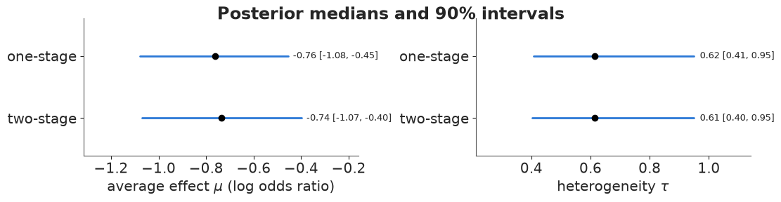
The two agree here because no trial is tiny and no cell is empty; when either fails, the one-stage model is the one to trust, and it is the one used from now on.
The forest plot, done properly
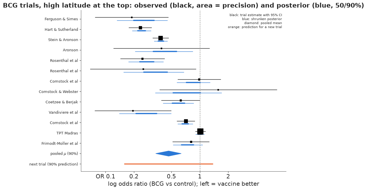
A forest plot shows each trial's own estimate and, in a Bayesian version, its shrunken posterior, then the pooled effect as a diamond. The line most forest plots omit is the prediction interval: where the effect of the next trial would fall. With $\tau$ this large it is several times wider than the interval for $\mu$, and it is the interval a public-health official planning a new BCG programme actually needs.
def forest(ax, idata, names, y_obs, se_obs, prefix, order=None, title=""):
    TH = stacked(idata.posterior[prefix + "theta"])
    MU = stacked(idata.posterior[prefix + "mu"])
    NEW = stacked(idata.posterior[prefix + "theta_new"])
    order = np.arange(len(names)) if order is None else order
    yy = np.arange(len(names))[::-1] + 2
    for row, i in zip(yy, order):
        ax.plot([y_obs[i] - 1.96 * se_obs[i], y_obs[i] + 1.96 * se_obs[i]], [row + 0.15, row + 0.15], color="k", lw=1)
        ax.scatter(y_obs[i], row + 0.15, color="k", s=8 + 200 / se_obs[i]**2 / (1 / se_obs**2).max(), marker="s", zorder=3)
        lo, q1, q3, hi = np.quantile(TH[:, i], [0.05, 0.25, 0.75, 0.95])
        ax.plot([lo, hi], [row - 0.15, row - 0.15], color=BLUE, lw=1)
        ax.plot([q1, q3], [row - 0.15, row - 0.15], color=BLUE, lw=3)
    lo, med, hi = np.quantile(MU, [0.05, 0.5, 0.95])
    ax.fill([lo, med, hi, med], [1, 1.25, 1, 0.75], color=BLUE)
    plo, phi = np.quantile(NEW, [0.05, 0.95])
    ax.plot([plo, phi], [0, 0], color=ORANGE, lw=2.5)
    ax.axvline(0, color=GREY, lw=1, ls="--")
    ax.set(yticks=np.r_[yy, 1, 0], xlabel="log odds ratio (BCG vs control); left = vaccine better", title=title)
    ax.set_yticklabels(list(np.asarray(names)[order]) + ["pooled $\\mu$ (90%)", "next trial (90% prediction)"], fontsize=9)
    ax.set_xticks(np.log([0.1, 0.2, 0.5, 1, 2]))
    ax.set_xticklabels(["OR 0.1", "0.2", "0.5", "1", "2"])
    return ax


fig, ax = plt.subplots(figsize=(9, 6.5))
forest(ax, idata_1, coords["trial"], y, se, "one_stage::", order=order[::-1],
       title="BCG trials, high latitude at the top: observed (black, area = precision) and posterior (blue, 50/90%)")
ax.text(0.98, 0.98, "black: trial estimate with 95% CI\nblue: shrunken posterior\ndiamond: pooled mean\norange: prediction for a new trial",
        transform=ax.transAxes, fontsize=8, va="top", ha="right");
3 · Heterogeneity is the result, not a nuisance
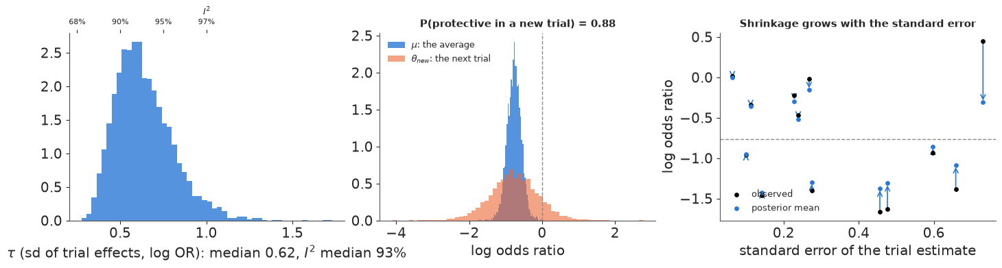
$\tau$ is usually reported once and then ignored. Three displays that make it speak:
- $\tau$ and $I^2$ as posteriors. $I^2$ is the share of the variation in observed effects that is heterogeneity rather than sampling noise; it is a function of $\tau$ and the trials' precisions, so it has a posterior too.
- The next trial. The predictive distribution of $\theta_{\text{new}}$ against the posterior of $\mu$: the first is what happens somewhere new, the second is a population average nobody will ever observe.
- Shrinkage against precision. How far each trial is pulled towards the mean, plotted against its standard error: imprecise trials move a long way, precise ones barely.
w = 1 / se**2
s2_typical = (K - 1) * w.sum() / (w.sum()**2 - (w**2).sum())  # Higgins & Thompson's typical within-trial variance
TAU = stacked(idata_1.posterior["one_stage::tau"])
MU = stacked(idata_1.posterior["one_stage::mu"])
NEW = stacked(idata_1.posterior["one_stage::theta_new"])
I2 = TAU**2 / (TAU**2 + s2_typical)
TH_mean = stacked(idata_1.posterior["one_stage::theta"]).mean(0)

fig, axes = plt.subplots(1, 3, figsize=(14, 3.8))
axes[0].hist(TAU, bins=50, color=BLUE, alpha=0.8, density=True)
axes[0].set(xlabel=f"$\\tau$ (sd of trial effects, log OR): median {np.median(TAU):.2f}, $I^2$ median {np.median(I2):.0%}")
ax2 = axes[0].twiny()
ax2.set_xlim(axes[0].get_xlim())
tau_ticks = np.array([0.25, 0.5, 0.75, 1.0])
ax2.set_xticks(tau_ticks)
ax2.set_xticklabels([f"{t**2 / (t**2 + s2_typical):.0%}" for t in tau_ticks], fontsize=8)
ax2.set_xlabel("$I^2$", fontsize=9)

axes[1].hist(MU, bins=60, color=BLUE, alpha=0.8, density=True, label="$\\mu$: the average")
axes[1].hist(NEW, bins=60, color=ORANGE, alpha=0.6, density=True, label="$\\theta_{new}$: the next trial")
axes[1].axvline(0, color=GREY, ls="--", lw=1)
axes[1].set(xlabel="log odds ratio")
axes[1].set_title(f"P(protective in a new trial) = {(NEW < 0).mean():.2f}", fontsize=11)
axes[1].legend(fontsize=9)

for i in range(K):
    axes[2].annotate("", xy=(se[i], TH_mean[i]), xytext=(se[i], y[i]),
                     arrowprops=dict(arrowstyle="->", color=BLUE, lw=1.2))
axes[2].scatter(se, y, color="k", s=15, zorder=3, label="observed")
axes[2].scatter(se, TH_mean, color=BLUE, s=15, zorder=3, label="posterior mean")
axes[2].axhline(np.median(MU), color=GREY, ls="--", lw=1)
axes[2].set(xlabel="standard error of the trial estimate", ylabel="log odds ratio")
axes[2].set_title("Shrinkage grows with the standard error", fontsize=11)
axes[2].legend(fontsize=9, loc="lower left");
4 · Meta-regression: explaining the heterogeneity
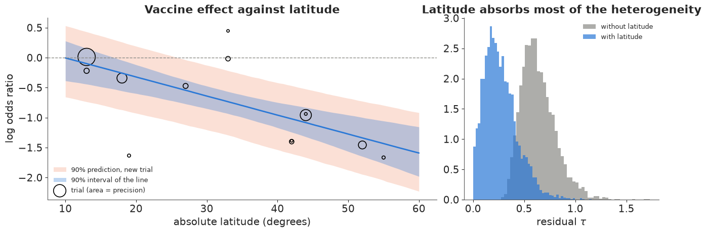
A study-level covariate turns $\mu$ into a line: $\theta_k = \mu + \beta\,(\text{lat}_k - \overline{\text{lat}}) + \tau z_k$. If latitude explains the differences between trials, the residual $\tau$ shrinks. The bubble plot (area = precision) is the standard display; the two bands are, again, the line and the prediction for a new trial at that latitude.
lat_c = (bcg.ablat - bcg.ablat.mean()).to_numpy(float)
metareg = one_stage_model(a, a + b, c, c + d, coords["trial"],
                          extra=lambda m: pm.Normal("beta", 0, 0.1) * lat_c)
idata_r = fit(metareg)
BETA = stacked(idata_r.posterior["one_stage::beta"])
MU_r = stacked(idata_r.posterior["one_stage::mu"])
TAU_r = stacked(idata_r.posterior["one_stage::tau"])
print(f"beta: {np.median(BETA):.3f} per degree of latitude, 90% [{np.quantile(BETA, 0.05):.3f}, {np.quantile(BETA, 0.95):.3f}]")
print(f"tau: {np.median(TAU):.2f} -> {np.median(TAU_r):.2f} with latitude in the model")

lat_grid = np.linspace(10, 60, 100)
line = MU_r[:, None] + BETA[:, None] * (lat_grid - bcg.ablat.mean())
new = line + TAU_r[:, None] * rng.normal(size=(len(MU_r), 1))
fig, axes = plt.subplots(1, 2, figsize=(13, 4.5), gridspec_kw={"width_ratios": [2, 1]})
ax = axes[0]
ax.fill_between(lat_grid, *np.quantile(new, [0.05, 0.95], axis=0), color=ORANGE, alpha=0.2, lw=0, label="90% prediction, new trial")
ax.fill_between(lat_grid, *np.quantile(line, [0.05, 0.95], axis=0), color=BLUE, alpha=0.3, lw=0, label="90% interval of the line")
ax.plot(lat_grid, np.median(line, axis=0), color=BLUE, lw=2)
ax.scatter(bcg.ablat, y, s=600 * w / w.max() + 10, facecolor="none", edgecolor="k", lw=1.2, label="trial (area = precision)")
ax.axhline(0, color=GREY, ls="--", lw=1)
ax.set(xlabel="absolute latitude (degrees)", ylabel="log odds ratio", title="Vaccine effect against latitude")
ax.legend(fontsize=9, loc="lower left")
axes[1].hist(TAU, bins=50, color=GREY, alpha=0.7, density=True, label="without latitude")
axes[1].hist(TAU_r, bins=50, color=BLUE, alpha=0.7, density=True, label="with latitude")
axes[1].set(xlabel="residual $\\tau$", title="Latitude absorbs most of the heterogeneity")
axes[1].legend(fontsize=9);
  one_stage: divergences = 2
beta: -0.031 per degree of latitude, 90% [-0.043, -0.018]
tau: 0.62 -> 0.24 with latitude in the model
5 · Which trials drive the answer, and when did we know?
Two questions a reviewer always asks, both answered by refitting. Leave-one-out influence: drop each trial and refit - which trial, if removed, moves $\mu$ the most? Cumulative meta-analysis: add trials in the order they were published - when did the evidence become conclusive, and did the later trials change the picture? With a one-stage model that fits in two seconds, 25 refits are cheap.
def mu_summary(idata):
    m = stacked(idata.posterior["one_stage::mu"])
    return np.quantile(m, [0.05, 0.5, 0.95]), (m < 0).mean()


loo_rows = []
for k in range(K):
    keep = np.arange(K) != k
    m_k = one_stage_model(a[keep], (a + b)[keep], c[keep], (c + d)[keep], coords["trial"][keep])
    with m_k:
        id_k = pm.sample(target_accept=0.95, random_seed=RANDOM_SEED, progressbar=False)
    loo_rows.append((bcg.author[k], *mu_summary(id_k)))

by_year = np.argsort(bcg.year.to_numpy(), kind="stable")
cum_rows = []
for n_trials in range(2, K + 1):
    keep = by_year[:n_trials]
    m_k = one_stage_model(a[keep], (a + b)[keep], c[keep], (c + d)[keep], coords["trial"][keep])
    with m_k:
        id_k = pm.sample(target_accept=0.95, random_seed=RANDOM_SEED, progressbar=False)
    cum_rows.append((bcg.year.to_numpy()[keep[-1]], bcg.author[keep[-1]], *mu_summary(id_k)))
full_lo, full_med, full_hi = np.quantile(MU, [0.05, 0.5, 0.95])
fig, axes = plt.subplots(1, 2, figsize=(14, 5.5))
ax = axes[0]
for row, (name, (lo, med, hi), p_neg) in enumerate(loo_rows[::-1]):
    ax.plot([lo, hi], [row, row], color=BLUE, lw=2)
    ax.scatter(med, row, color="k", zorder=3, s=20)
ax.axvspan(full_lo, full_hi, color=GREY, alpha=0.2, lw=0)
ax.axvline(full_med, color=GREY, lw=1)
ax.set(yticks=range(K), xlabel="pooled $\\mu$ with this trial removed (90%)", title="Leave-one-out influence")
ax.set_yticklabels([f"without {r[0]}" for r in loo_rows[::-1]], fontsize=9)

ax = axes[1]
for row, (year, name, (lo, med, hi), p_neg) in enumerate(cum_rows):
    ax.plot([lo, hi], [row, row], color=BLUE, lw=2)
    ax.scatter(med, row, color="k", zorder=3, s=20)
    ax.text(hi + 0.05, row, f"P($\\mu$<0) = {p_neg:.2f}", va="center", fontsize=8)
ax.axvline(0, color=GREY, lw=1, ls="--")
ax.set(yticks=range(len(cum_rows)), xlabel="pooled $\\mu$ after each trial was published (90%)",
       title="Cumulative meta-analysis by year", xlim=(-2.2, 1.2))
ax.set_yticklabels([f"{r[0]}: + {r[1]}" for r in cum_rows], fontsize=9)
ax.invert_yaxis();
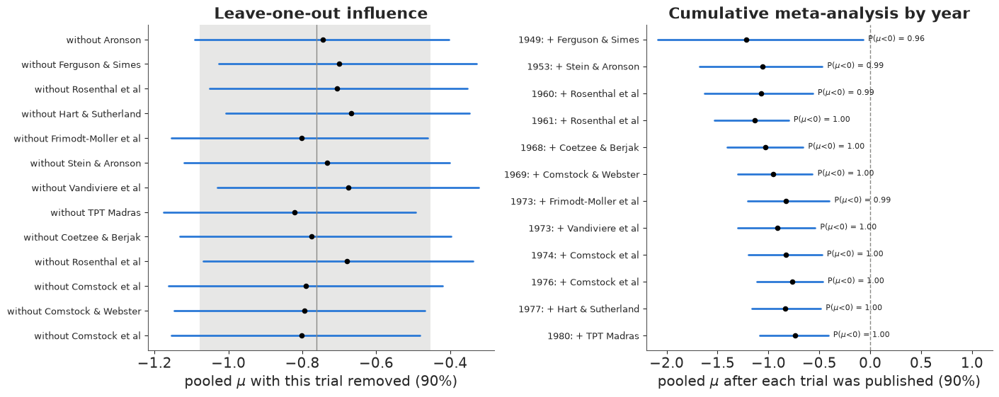
Read the left panel against the grey band (the full-data posterior): no single trial moves the pooled estimate outside it, which is the reassurance one wants. Read the right panel top to bottom: the case for the vaccine was already strong by the early 1950s, and the 177,000-participant Madras trial of 1980 (odds ratio 1.0) pulled the average towards zero without coming close to overturning it - the random-effects model treats it as one more setting, not as the final word.
6 · What the database cannot tell you: small-study effects
A database of published studies has a blind spot: studies that were never published. The classic demonstration is intravenous magnesium after a heart attack. Through the early 1990s, a meta-analysis of small trials found a large mortality benefit, and a 1993 paper called it an "effective, safe, simple and inexpensive" treatment. Then ISIS-4 randomised 58,050 patients and found nothing. Egger et al. (2001) assembled the 16 trials to study what went wrong.
The funnel plot puts each trial's effect against its standard error, so precise trials sit at the top near the truth and imprecise ones fan out symmetrically below - if what was published is all that was run. A Bayesian Egger model adds a term $\gamma\,s_k$ to the trial effect: $\gamma$ is the small-study slope, and $\mu$ becomes the effect a trial of infinite precision would find.
data.describe("magnesium")
mg = data.load("magnesium")
a2, n1, c2, n2 = (mg[col].to_numpy(float) for col in ["ai", "n1i", "ci", "n2i"])
cc = 0.5 * ((a2 == 0) | (c2 == 0))               # continuity correction only where a cell is zero
y2 = np.log(((a2 + cc) / (n1 - a2 + cc)) / ((c2 + cc) / (n2 - c2 + cc)))
se2 = np.sqrt(1 / (a2 + cc) + 1 / (n1 - a2 + cc) + 1 / (c2 + cc) + 1 / (n2 - c2 + cc))
mg_names = mg.study.to_numpy(dtype=object)


def normal_re(y_, se_, names, slope=None, name="re"):
    with pm.Model(coords={"trial": names}, name=name) as m:
        mu = pm.Normal("mu", 0, 1.5)
        tau = pm.HalfNormal("tau", 1)
        z = pm.Normal("z", 0, 1, dims="trial")
        shift = pm.Normal("gamma", 0, 2) * slope if slope is not None else 0.0
        pm.Normal("y", mu + shift + tau * z, se_, observed=y_, dims="trial")
    return m


id_all = fit(normal_re(y2, se2, mg_names, name="all16"))
id_small = fit(normal_re(y2[:-1], se2[:-1], mg_names[:-1], name="without_ISIS4"))
id_egger = fit(normal_re(y2, se2, mg_names, slope=se2, name="egger"))
GAMMA = stacked(id_egger.posterior["egger::gamma"])
print(f"small-study slope gamma: median {np.median(GAMMA):.2f}, P(gamma < 0) = {(GAMMA < 0).mean():.3f}")
magnesium: 16 trials: deaths and patients per arm, including the 58,050-patient ISIS-4 mega-trial.
  source: Egger, Davey Smith & Altman (2001), intravenous magnesium after myocardial infarction, via `metadat`.
  url:    https://raw.githubusercontent.com/wviechtb/metadat/master/data-raw/dat.egger2001.txt
all16: divergences = 0
without_ISIS4: divergences = 0
  egger: divergences = 14
small-study slope gamma: median -1.35, P(gamma < 0) = 0.998
fig, axes = plt.subplots(1, 2, figsize=(14, 5.5), gridspec_kw={"width_ratios": [1.3, 1]})
ax = axes[0]
se_grid = np.linspace(0.01, 1.8, 100)
# contour-enhanced funnel (Peters et al. 2008): shade where a trial with this SE is "significant",
# darker for smaller p; the central white wedge is p > 0.1. Missing trials in the white wedge = suspicious.
z_cuts = [stats.norm.ppf(1 - p / 2) for p in (0.1, 0.05, 0.01)] + [np.inf]
for (z_lo, z_hi), shade in zip(zip(z_cuts[:-1], z_cuts[1:]), (0.08, 0.16, 0.26)):
    for sign in (-1, 1):
        ax.fill_betweenx(se_grid, sign * z_lo * se_grid, np.clip(sign * z_hi * se_grid, -5, 5), color="k", alpha=shade, lw=0)
mu_all, tau_all = np.median(stacked(id_all.posterior["all16::mu"])), np.median(stacked(id_all.posterior["all16::tau"]))
ax.plot(mu_all - 1.96 * np.sqrt(se_grid**2 + tau_all**2), se_grid, color=BLUE, ls="--", lw=1.2)
ax.plot(mu_all + 1.96 * np.sqrt(se_grid**2 + tau_all**2), se_grid, color=BLUE, ls="--", lw=1.2, label="random-effects 95% funnel")
mu_e = np.median(stacked(id_egger.posterior["egger::mu"]))
ax.plot(mu_e + np.median(GAMMA) * se_grid, se_grid, color=ORANGE, lw=2, label="Egger line: effect drifts with SE")
ax.scatter(y2, se2, color="k", s=30, zorder=3)
for j in [13, 15]:
    ax.annotate(mg_names[j], (y2[j], se2[j]), xytext=(8, -4), textcoords="offset points", fontsize=9)
ax.invert_yaxis()
ax.set(xlabel="log odds ratio (magnesium vs control); left = fewer deaths", ylabel="standard error (precise trials at the top)",
       xlim=(-5, 5))
ax.set_title("Contour-enhanced funnel: grey = 'significant' at 10% / 5% / 1%, white = not", fontsize=11)
ax.legend(fontsize=9, loc="lower left")

ax = axes[1]
for idata, pre, col, lab in [(id_small, "without_ISIS4::", GREY, "15 small trials only"),
                             (id_all, "all16::", BLUE, "all 16, random effects"),
                             (id_egger, "egger::", ORANGE, "Egger-adjusted: $\\mu$ at SE = 0")]:
    ax.hist(stacked(idata.posterior[pre + "mu"]), bins=60, density=True, alpha=0.6, color=col, label=lab)
ax.axvline(y2[-1], color="k", lw=2, label=f"ISIS-4 alone: {y2[-1]:+.2f}")
ax.set(xlabel="pooled log odds ratio")
ax.set_title("Three answers to 'does magnesium save lives?'", fontsize=11)
ax.legend(fontsize=9);
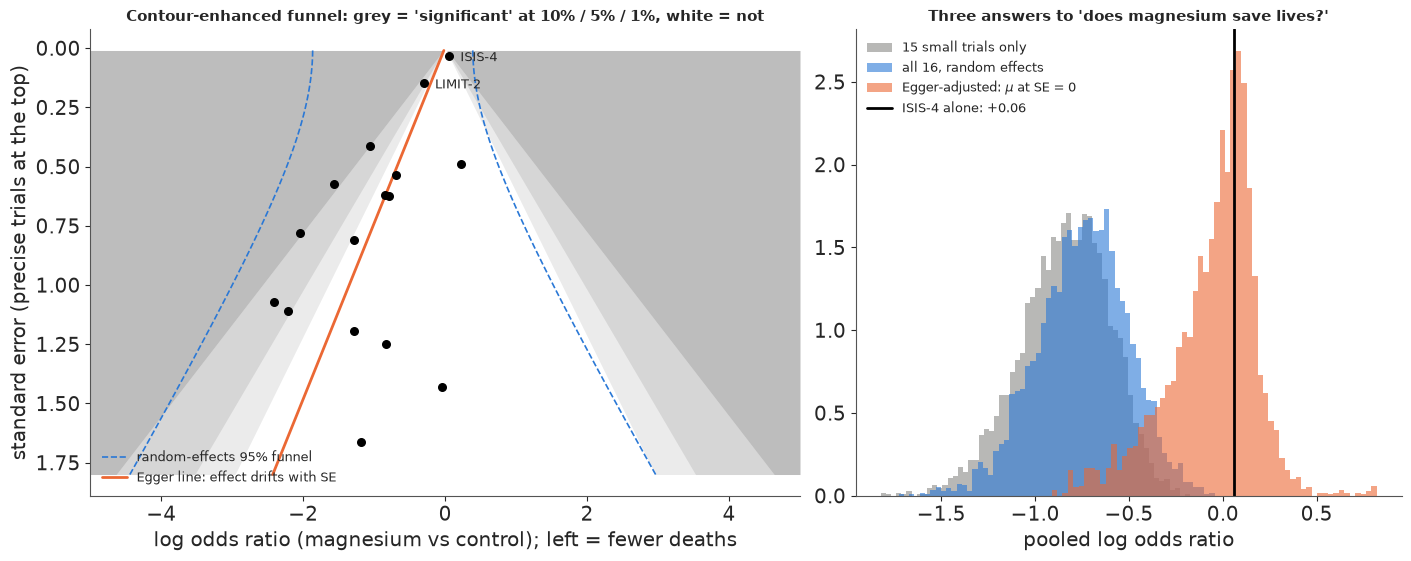
The small trials sit almost entirely in the lower-left: the imprecise ones all found large benefits, exactly the asymmetry a mix of publication bias and small-trial quality problems produces, and the slope $\gamma$ is decisively negative. The random-effects model on all 16 trials still says "magnesium halves mortality" because it treats ISIS-4 as one trial among many; the Egger-adjusted $\mu$ says "no effect", which is what ISIS-4 found. Neither model knows which is right - the adjustment is a hypothesis about the missing studies - but a funnel this lopsided is the database telling you what it does not contain.
7 · When the database protects privacy harder than it needs to
Section 1 showed that releasing the counts costs nothing. Real data custodians often go further, because a count of 1 in a small cell can be identifying when combined with other releases. Two common mechanisms, and how to model each so the analysis stays honest:
7.1 Small-cell suppression: "fewer than 10"
Cells below a threshold are published as "<10". A suppressed cell is not missing, it is
interval-censored: we know the count is in $\{0, \ldots, 9\}$. pm.Censored around the
Binomial does exactly this: an observation at the bound contributes $P(X \le 9)$ instead of
$P(X = x)$.
THR = 10
suppressed_t, suppressed_c = a < THR, c < THR
print(f"cells published as '<{THR}': {suppressed_t.sum()} BCG-arm and {suppressed_c.sum()} control-arm counts "
      f"({', '.join(bcg.author[suppressed_t | suppressed_c])})")

with pm.Model(coords=coords, name="suppressed") as suppressed:
    mu = pm.Normal("mu", 0, 1.5)
    tau = pm.HalfNormal("tau", 1)
    z = pm.Normal("z", 0, 1, dims="trial")
    theta = pm.Deterministic("theta", mu + tau * z, dims="trial")
    alpha = pm.Normal("alpha", -4, 2, dims="trial")
    # lower=THR-1 where suppressed: an observed value of THR-1 then means "at most THR-1"
    pm.Censored("cases_c", pm.Binomial.dist(n=c + d, p=pm.math.invlogit(alpha)),
                lower=np.where(suppressed_c, THR - 1, -1), upper=None,
                observed=np.where(suppressed_c, THR - 1, c), dims="trial")
    pm.Censored("cases_t", pm.Binomial.dist(n=a + b, p=pm.math.invlogit(alpha + theta)),
                lower=np.where(suppressed_t, THR - 1, -1), upper=None,
                observed=np.where(suppressed_t, THR - 1, a), dims="trial")
    pm.Deterministic("theta_new", mu + tau * pm.Normal("z_new", 0, 1))
idata_s = fit(suppressed)
cells published as '<10': 5 BCG-arm and 1 control-arm counts (Aronson, Ferguson & Simes, Rosenthal et al, Vandiviere et al, Comstock & Webster)
suppressed: divergences = 1
TH_full = stacked(idata_1.posterior["one_stage::theta"])
TH_sup = stacked(idata_s.posterior["suppressed::theta"])
fig, ax = plt.subplots(figsize=(9, 5.5))
yy = np.arange(K)[::-1]
for row, i in zip(yy, order):
    for S, off, col in [(TH_full, 0.18, BLUE), (TH_sup, -0.18, ORANGE)]:
        lo, q1, q3, hi = np.quantile(S[:, i], [0.05, 0.25, 0.75, 0.95])
        ax.plot([lo, hi], [row + off, row + off], color=col, lw=1)
        ax.plot([q1, q3], [row + off, row + off], color=col, lw=3)
    if suppressed_t[i] or suppressed_c[i]:
        ax.text(1.05, row, f"'<{THR}'", color=ORANGE, fontsize=9, va="center")
ax.axvline(0, color=GREY, lw=1, ls="--")
ax.set(yticks=yy, xlabel="log odds ratio", xlim=(-2.6, 1.3),
       title="Trial posteriors from the full counts (blue) and with small cells suppressed (orange)")
ax.set_yticklabels(list(coords["trial"][order]), fontsize=9)
for pre, idata, lab in [("one_stage::", idata_1, "full counts"), ("suppressed::", idata_s, "suppressed")]:
    m = stacked(idata.posterior[pre + "mu"])
    print(f"{lab:12s} mu = {np.median(m):.2f} [{np.quantile(m, 0.05):.2f}, {np.quantile(m, 0.95):.2f}]   "
          f"tau = {np.median(stacked(idata.posterior[pre + 'tau'])):.2f}")
full counts  mu = -0.76 [-1.08, -0.45]   tau = 0.62
suppressed   mu = -0.84 [-1.33, -0.47]   tau = 0.69
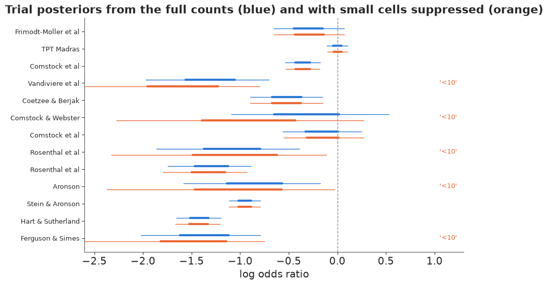
Suppression widens the affected trials' posteriors a lot and the pooled interval a little (its lower end moves from -1.1 to -1.3; the median by less than 0.1): the cells under 10 belong to the small trials, which carried little weight to begin with. The important thing is what did not happen: a censored likelihood does not bias the estimate, whereas treating "<10" as 9, or as 5, or dropping those trials, would.
7.2 Differential privacy: calibrated noise on every count
Differential privacy gives a formal guarantee - the released numbers are almost equally likely whether or not any one person took part - by adding noise before release. With the Gaussian mechanism, each case count gets $\text{Normal}(0, \sigma_{\text{DP}})$ noise with $\sigma_{\text{DP}} = \sqrt{2\ln(1.25/\delta)}\,/\,\varepsilon$; smaller $\varepsilon$ means stronger privacy and more noise. (The enrolment totals are treated as public.)
The released count is then $\tilde{x}_k = x_k + e_k$, and the analyst's model must include $e_k$. A count is approximately $\text{Normal}(np,\ np(1-p))$, and adding independent noise just adds $\sigma_{\text{DP}}^2$ to that variance, so the noise-aware model is one line different from a naive one that pretends the noisy counts are exact. We sweep $\varepsilon$ from generous to strict, with one noise draw per level, and fit both models.
DELTA = 1e-5
epsilons = np.array([4, 2, 1, 0.5, 0.25, 0.1])
sigmas = np.sqrt(2 * np.log(1.25 / DELTA)) / epsilons


def dp_model(noisy_t, noisy_c, sigma_dp, aware):
    with pm.Model(coords=coords, name="dp_aware" if aware else "dp_naive") as m:
        mu = pm.Normal("mu", 0, 1.5)
        tau = pm.HalfNormal("tau", 1)
        z = pm.Normal("z", 0, 1, dims="trial")
        theta = pm.Deterministic("theta", mu + tau * z, dims="trial")
        alpha = pm.Normal("alpha", -4, 2, dims="trial")
        p_c, p_t = pm.math.invlogit(alpha), pm.math.invlogit(alpha + theta)
        extra = sigma_dp**2 if aware else 0.0
        pm.Normal("cases_c", (c + d) * p_c, pm.math.sqrt((c + d) * p_c * (1 - p_c) + extra), observed=noisy_c, dims="trial")
        pm.Normal("cases_t", (a + b) * p_t, pm.math.sqrt((a + b) * p_t * (1 - p_t) + extra), observed=noisy_t, dims="trial")
    return m


dp_results = []
for eps, sig in zip(epsilons, sigmas):
    noisy_t, noisy_c = a + rng.normal(0, sig, K), c + rng.normal(0, sig, K)
    print(f"epsilon = {eps:<5} sigma_DP = {sig:5.1f}", end="")
    row = {"eps": eps, "sigma": sig}
    for aware in (True, False):
        with dp_model(noisy_t, noisy_c, sig, aware):
            id_dp = pm.sample(target_accept=0.95, random_seed=RANDOM_SEED, progressbar=False)
        pre = "dp_aware::" if aware else "dp_naive::"
        row["aware" if aware else "naive"] = np.quantile(stacked(id_dp.posterior[pre + "mu"]), [0.05, 0.5, 0.95])
        row[("aware" if aware else "naive") + "_theta_sd"] = stacked(id_dp.posterior[pre + "theta"]).std(0)
        print(f"   {'aware' if aware else 'naive'} div = {int(id_dp.sample_stats['diverging'].sum())}", end="")
    print()
    dp_results.append(row)
epsilon = 4.0 sigma_DP = 1.2
aware div = 0
   naive div = 0
epsilon = 2.0   sigma_DP =   2.4
aware div = 0
   naive div = 0
epsilon = 1.0   sigma_DP =   4.8
aware div = 0
   naive div = 0
epsilon = 0.5   sigma_DP =   9.7
aware div = 0
   naive div = 0
epsilon = 0.25  sigma_DP =  19.4
aware div = 0
   naive div = 0
epsilon = 0.1   sigma_DP =  48.4
aware div = 0
naive div = 0
fig, axes = plt.subplots(1, 2, figsize=(14, 5))
ax = axes[0]
x = np.arange(len(epsilons))
ax.axhspan(full_lo, full_hi, color=GREY, alpha=0.2, lw=0, label="no privacy: full counts (90%)")
ax.axhline(full_med, color=GREY, lw=1)
for key, col, off, lab in [("aware", BLUE, -0.1, "noise-aware model"), ("naive", ORANGE, 0.1, "naive model (ignores the noise)")]:
    lo, med, hi = np.array([r[key] for r in dp_results]).T
    ax.errorbar(x + off, med, yerr=[med - lo, hi - med], fmt="o", color=col, capsize=3, label=lab)
ax.axhline(0, color="k", lw=0.8, ls=":")
ax.set(xticks=x, xticklabels=[f"$\\varepsilon$ = {e}\n$\\sigma$ = {s:.0f}" for e, s in zip(epsilons, sigmas)],
       ylabel="pooled $\\mu$ (90%)")
ax.set_title("Privacy-utility: stronger privacy to the right", fontsize=11)
ax.legend(fontsize=9, loc="upper left")

ax = axes[1]
n_cases = a + c                                   # what the noise competes with: the number of events
cmap = plt.get_cmap("Blues")
label_these = np.r_[np.argsort(n_cases)[:2], np.argsort(n_cases)[-3:]]
for i in np.argsort(n_cases):
    sd_path = [r["aware_theta_sd"][i] for r in dp_results]
    ax.plot(x, sd_path, marker="o", ms=4, lw=1.5, color=cmap(0.3 + 0.7 * np.log(n_cases[i]) / np.log(n_cases.max())))
    if i in label_these:
        ax.text(x[-1] + 0.1, sd_path[-1], f"{coords['trial'][i]}: {int(n_cases[i])} cases", fontsize=8, va="center")
ax.set(xticks=x, xticklabels=[f"$\\varepsilon$ = {e}" for e in epsilons], ylabel="posterior sd of the trial effect $\\theta_k$",
       xlim=(-0.3, len(x) + 1.6))
ax.set_title("Which trials still carry information (darker = more cases)", fontsize=11);
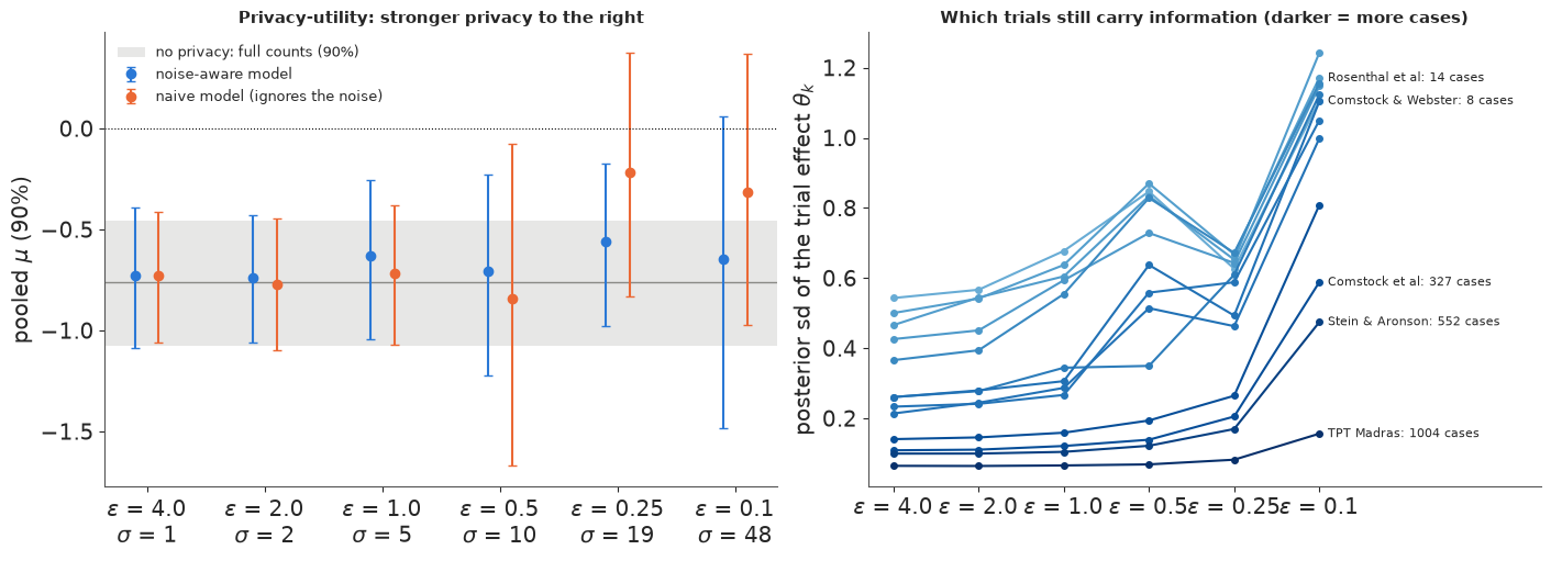
Two lessons, one for each panel. Left: the naive analysis does not merely get noisier as privacy tightens - its estimate drifts towards no effect (noise added to a count of 4 cases reads as a weaker contrast: the classical attenuation of measurement error), and its interval has no way of knowing that. The noise-aware model stays centred near the full-data answer at every $\varepsilon$ and widens instead: its interval is the price of the privacy, stated in the units of the question. Right: what protects a trial from the noise is its number of cases, not its number of participants. Tuberculosis is rare, so a trial of 26,000 people may hold only 62 cases and lose most of its precision at $\varepsilon \le 0.25$; only Madras, with a thousand cases, is nearly untouched. A database that adds noise should say so in its metadata, because the analyst can account for it - but only if told.
(One noise realisation per $\varepsilon$ is enough to make the point; a proper evaluation would average the curve over many draws of the noise. That is one of the exercises.)
8 · Studies inside studies: a three-level model
Many databases have structure above the study: trials from the same research group, sites within a multi-centre trial, or here 56 studies of modified school calendars nested in 11 school districts. Two variance components - between districts and between studies within a district - and the question of how much of the heterogeneity lives at each level.
data.describe("konstantopoulos")
ko = data.load("konstantopoulos")
districts = np.sort(ko.district.unique())
d_idx = pd.Index(districts).get_indexer(ko.district)

with pm.Model(coords={"district": districts.astype(str), "study": ko.study.to_numpy()}, name="three_level") as three_level:
    mu = pm.Normal("mu", 0, 1)
    tau_d = pm.HalfNormal("tau_district", 0.5)
    tau_s = pm.HalfNormal("tau_study", 0.5)
    delta = pm.Deterministic("delta", mu + tau_d * pm.Normal("zd", 0, 1, dims="district"), dims="district")
    theta = pm.Deterministic("theta", delta[d_idx] + tau_s * pm.Normal("zs", 0, 1, dims="study"), dims="study")
    pm.Normal("y", theta, np.sqrt(ko.vi.to_numpy()), observed=ko.yi.to_numpy(), dims="study")
    pm.Deterministic("icc", tau_d**2 / (tau_d**2 + tau_s**2))
idata_3 = fit(three_level)
az.summary(idata_3, var_names=["three_level::mu", "three_level::tau_district", "three_level::tau_study", "three_level::icc"],
           ci_kind="hdi", ci_prob=0.9, round_to=2)
konstantopoulos: 56 studies nested in 11 school districts: standardised mean difference, its variance, year.
  source: Konstantopoulos (2011), modified school calendars and achievement, via `metadat`.
  url:    https://raw.githubusercontent.com/wviechtb/metadat/master/data-raw/dat.konstantopoulos2011.txt
three_level: divergences = 0
| mean | sd | hdi90_lb | hdi90_ub | ess_bulk | ess_tail | r_hat | mcse_mean | mcse_sd | |
|---|---|---|---|---|---|---|---|---|---|
| three_level::mu | 0.18 | 0.09 | 0.03 | 0.33 | 372.67 | 590.93 | 1.02 | 0.00 | 0.0 |
| three_level::tau_district | 0.28 | 0.08 | 0.16 | 0.41 | 567.25 | 934.71 | 1.01 | 0.00 | 0.0 |
| three_level::tau_study | 0.19 | 0.03 | 0.13 | 0.24 | 894.87 | 1393.65 | 1.00 | 0.00 | 0.0 |
| three_level::icc | 0.66 | 0.15 | 0.43 | 0.89 | 598.82 | 1111.89 | 1.00 | 0.01 | 0.0 |
DELTA_ = stacked(idata_3.posterior["three_level::delta"])
TH3 = stacked(idata_3.posterior["three_level::theta"])
ICC = stacked(idata_3.posterior["three_level::icc"])
cmap = plt.get_cmap("tab20")
fig, axes = plt.subplots(1, 2, figsize=(14, 6), gridspec_kw={"width_ratios": [2.2, 1]})
ax = axes[0]
row = 0
for j, dname in enumerate(districts):
    members = np.where(d_idx == j)[0]
    col = cmap(j / len(districts))
    lo, hi = np.quantile(DELTA_[:, j], [0.05, 0.95])
    ax.fill_betweenx([row - 0.5, row + len(members) - 0.5], lo, hi, color=col, alpha=0.2, lw=0)
    ax.axvline(0, color=GREY, lw=1, ls="--")
    for s in members:
        yi, sei = ko.yi[s], np.sqrt(ko.vi[s])
        ax.plot([yi - 1.96 * sei, yi + 1.96 * sei], [row, row], color="k", lw=0.8, alpha=0.6)
        ax.plot(np.quantile(TH3[:, s], [0.05, 0.95]), [row, row], color=col, lw=2.5)
        row += 1
    ax.text(1.25, row - len(members) / 2 - 0.5, f"district {dname}", va="center", fontsize=8, color=col)
ax.set(yticks=[], xlim=(-1.2, 1.6), xlabel="standardised mean difference")
ax.set_title("56 studies in 11 districts: observed 95% CI (black), posterior 90% (colour), district mean (shaded)", fontsize=10)
ax.invert_yaxis()
axes[1].hist(ICC, bins=50, color=BLUE, alpha=0.8, density=True)
axes[1].set(xlabel="share of heterogeneity between districts", xlim=(0, 1))
axes[1].set_title(f"ICC: median {np.median(ICC):.2f}, 90% [{np.quantile(ICC, 0.05):.2f}, {np.quantile(ICC, 0.95):.2f}]", fontsize=11);
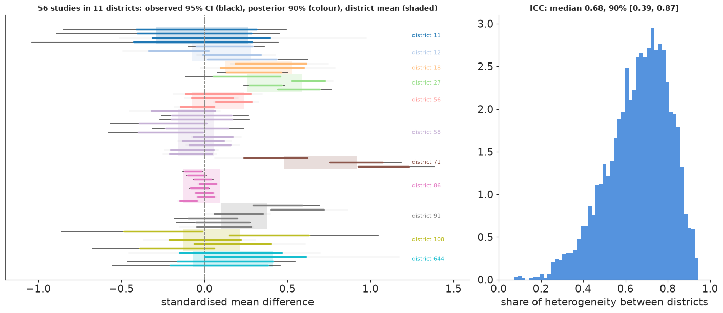
Most of the heterogeneity is between districts, not between studies within one: a study's result tells you more about its district than about the intervention in general, and a two-level model that ignored the districts would report a $\tau$ that mixes the two and an interval for $\mu$ that is too narrow (11 districts, not 56 studies, are the effective sample size for the top level).
9 · Summary
| Question | Display / model |
|---|---|
| What did each study find and what do we now believe about it? | forest plot: observed CI, shrunken posterior, pooled diamond, prediction interval |
| How different are the studies? | posterior of $\tau$ and $I^2$; the predictive distribution of a new trial |
| Why are they different? | meta-regression on a study-level covariate; residual $\tau$ |
| Does one study drive the answer? When did we know? | leave-one-out influence; cumulative meta-analysis |
| What is missing from the database? | contour-enhanced funnel; a small-study slope (Egger) |
| Studies within groups? | three-level model; ICC |
| Counts are all we get - do we lose anything? | no: they are sufficient statistics (section 1) |
| Counts are suppressed or noised - what then? | censored likelihood; noise-aware likelihood; measure the loss (section 7) |
Try it yourself
- Average over the noise. Repeat the $\varepsilon$ sweep of section 7.2 with ten noise draws per level and plot the mean and spread of the posterior sd of $\mu$ against $\varepsilon$. At what $\varepsilon$ does the noise-aware posterior first become wider than the "15 small trials only" magnesium posterior of section 6?
- The Laplace mechanism. Pure $\varepsilon$-DP adds Laplace($1/\varepsilon$) noise
instead of Gaussian. Write the noise-aware likelihood with a Laplace error term (a
pm.CustomDistof Binomial-normal-approximation plus Laplace, or a latent true count with a Normal approximation) and compare the two mechanisms at equal $\varepsilon$. - Magnesium in one stage. Refit section 6 with the binomial one-stage model and no continuity correction (the Bertschat trial has zero deaths in one arm). Does the Egger-type adjustment still say "no effect" when the slope is put on $\sqrt{1/n_k}$ instead of the estimated standard error?