Disease counts are rarely published per person or per coordinate. They are published per area: a district, a county, a postcode. Two neighbouring districts share a population that commutes, a coastline, an industry, a water supply, so their disease rates tend to be alike - but "neighbouring" is a statement about a map, not about a distance. Skye and the Western Isles are neighbours across a strait; Glasgow and one of its suburbs are neighbours across a street. The natural object is a graph: one node per area, an edge for "shares a border".
This notebook builds that graph from real polygons and puts the three classic graph priors on it: the intrinsic CAR (ICAR), the proper CAR, and BYM2, the modern default for disease mapping. It deliberately runs into the three problems that trip people up in practice - islands, a CAR parameter that will not leave the boundary, and a variance that means something different on every map - and fixes each one.
Why this dataset. The repository already has county polygons for the whole US (E16), and Minnesota radon (E02) sits on them. But radon is a set of home measurements, not areal counts, and fitting it with a county-level CAR would teach the wrong lesson. The Scottish lip-cancer data is the benchmark for areal models precisely because it is what these models are for: small counts with a known expected count per area, very unequal populations (from 1.4 to 88 expected cases), a covariate with a plausible mechanism (sunlight: outdoor work), real islands, and results that have been reproduced in WinBUGS, INLA, CARBayes and Stan, so we can check ours.
import json
import logging
import warnings

import arviz as az
import matplotlib.pyplot as plt
import numpy as np
import pandas as pd
import pymc as pm
from matplotlib.collections import LineCollection, PolyCollection
from matplotlib.colors import TwoSlopeNorm
from scipy import stats
from scipy.sparse.csgraph import connected_components
from scipy.special import logsumexp

from pymc_challenges import data

RANDOM_SEED = 1987
rng = np.random.default_rng(RANDOM_SEED)
az.style.use("arviz-variat")
logging.getLogger("pymc").setLevel(logging.WARNING)  # ~40 fits below: no banner per fit
BLUE, ORANGE, AQUA, GREY, RED = "#2a78d6", "#eb6834", "#1baf7a", "#8a8a86", "#c8374b"
print(f"PyMC {pm.__version__}, ArviZ {az.__version__}")
PyMC 6.3.2, ArviZ 1.3.0
1 · Question and data
Between 1975 and 1980, 536 men in Scotland were diagnosed with lip cancer. For each of the 56 districts we know the observed count $y_i$ and an expected count $E_i$: what the district would have seen if every age group had the national rate. Their ratio is the standardised morbidity ratio $\text{SMR}_i = y_i / E_i$, the raw estimate of the district's relative risk. The epidemiological question is twofold:
- Where is the risk genuinely elevated, once the noise of small counts is accounted for?
- Does outdoor work explain it? Lip cancer is linked to sunlight exposure, and
AFFis the percentage of the workforce in agriculture, fishing and forestry.
The data come as a GeoJSON of district polygons with the counts as properties.
data.describe("scotland_lip_geojson")
geo = json.load(open(data.path("scotland_lip_geojson")))
lip = pd.DataFrame([f["properties"] for f in geo["features"]])
rings = [np.asarray(f["geometry"]["coordinates"][0]) for f in geo["features"]]  # outer rings
print({f["geometry"]["type"] for f in geo["features"]}, "- coordinates in metres (British National Grid)")
lip = lip.rename(columns={"NAME": "district", "CANCER": "y", "CEXP": "E"})
lip["SMR"] = lip.y / lip.E
N = len(lip)
names = lip.district.to_numpy(dtype=object)
y, E = lip.y.to_numpy(), lip.E.to_numpy()
aff = lip.AFF.to_numpy(float)
lip[["district", "y", "E", "SMR", "AFF", "POP"]].sort_values("SMR").iloc[[0, 1, 2, 27, 28, -3, -2, -1]].round(2)
scotland_lip_geojson: 56 Scottish districts (British National Grid polygons, metres) with observed cases CANCER, expected cases CEXP, population POP and % in agriculture/fishing/forestry AFF. GeoJSON: use data.path().
  source: Clayton & Kaldor (1987) male lip cancer 1975-80 via Cressie (1993); expected counts and AFF from Lawson et al. (1999); WinBUGS boundaries prepared by Luc Anselin for the GeoDa Center data-and-lab.
  url:    https://geodacenter.github.io/data-and-lab/data/scotlip.zip
{'Polygon'} - coordinates in metres (British National Grid)| district | y | E | SMR | AFF | POP | |
|---|---|---|---|---|---|---|
| 55 | Annandale | 0 | 1.76 | 0.00 | 10 | 103412 |
| 54 | Tweeddale | 0 | 4.16 | 0.00 | 16 | 38704 |
| 53 | Strathkelvin | 1 | 7.03 | 0.14 | 1 | 246744 |
| 28 | Perth-Kinross | 16 | 14.37 | 1.11 | 10 | 346041 |
| 27 | EastLothian | 10 | 8.96 | 1.12 | 7 | 231185 |
| 2 | Caithness | 11 | 3.04 | 3.62 | 10 | 83190 |
| 1 | Banff-Buchan | 39 | 8.66 | 4.50 | 16 | 231337 |
| 0 | Skye-Lochalsh | 9 | 1.38 | 6.52 | 16 | 28324 |
Every geometry is a single polygon (GeoDa merged multi-part islands into one ring), with
coordinates on the British National Grid - metres on a flat projection, so an aspect ratio
of 1 draws Scotland without distortion. A choropleth needs no GIS library: a
PolyCollection of the rings coloured by value (as in E16).
def draw_map(ax, values, cmap="viridis", norm=None, title="", cbar_label="", edges=None, **kw):
    pc = PolyCollection(rings, array=np.asarray(values, float), cmap=cmap, norm=norm,
                        edgecolor="white", linewidth=0.4, **kw)
    ax.add_collection(pc)
    if edges is not None:
        ax.add_collection(edges)
    ax.autoscale_view()
    ax.set_aspect(1)
    ax.set_axis_off()
    ax.set_title(title, fontsize=11)
    plt.colorbar(pc, ax=ax, shrink=0.6, label=cbar_label)
    return pc


RR_NORM = TwoSlopeNorm(vcenter=0.0, vmin=np.log(0.2), vmax=np.log(5))  # log relative risk, centred at RR = 1


def rr_colorbar_ticks(pc):
    ticks = [0.2, 0.5, 1, 2, 5]
    pc.colorbar.set_ticks(np.log(ticks))
    pc.colorbar.set_ticklabels([str(t) for t in ticks])


fig, axes = plt.subplots(1, 3, figsize=(15, 6.5))
draw_map(axes[0], np.log(E), cmap="Greys", title="expected cases $E_i$ (log scale)", cbar_label="log E")
pc = draw_map(axes[1], np.log(np.clip(lip.SMR, 0.2, None)), cmap="RdBu_r", norm=RR_NORM,
              title="raw SMR = observed / expected", cbar_label="SMR")
rr_colorbar_ticks(pc)
draw_map(axes[2], aff, cmap="YlGn", title="AFF: % outdoor workforce", cbar_label="%");
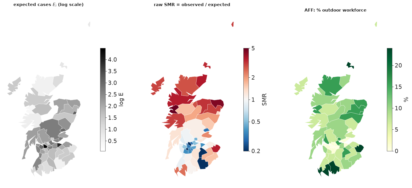
The raw SMR map shows the pattern that made this dataset famous: high ratios in the north and west (the Highlands, Skye, the islands), ratios below 1 in the urban central belt. The outdoor-work map has a similar shape. Two warnings, though. First, the most extreme SMRs belong to the smallest districts (Skye-Lochalsh: 9 cases where 1.4 were expected), and the two districts with zero cases expected fewer than 5 - their SMR of 0 is mostly noise. Second, AFF and the risk share their spatial pattern, so any model that lets the risk vary smoothly in space will compete with AFF to explain the same map. Both themes run through the rest of the notebook.
2 · From polygons to a graph
Two districts are queen neighbours if their boundaries share at least one point, and rook neighbours if they share at least one boundary segment (the names come from chess: a rook cannot move diagonally across a corner). Topological shapefiles like this one store a shared border with identical vertices on both sides, so a set intersection of vertex keys does the job; rounding the coordinates to a tolerance first makes the same code work on files whose borders were digitised twice.
def contiguity(rings, tol=1.0, rule="queen"):
    """Adjacency matrix from polygon rings: shared vertices (queen) or shared edges (rook)."""
    keys = [[tuple(k) for k in np.round(r / tol).astype(np.int64)] for r in rings]
    if rule == "queen":
        sets = [set(k[:-1]) for k in keys]
    else:
        sets = [{frozenset(e) for e in zip(k[:-1], k[1:]) if e[0] != e[1]} for k in keys]
    n = len(rings)
    W = np.zeros((n, n), dtype=int)
    for i in range(n):
        for j in range(i + 1, n):
            W[i, j] = W[j, i] = len(sets[i] & sets[j]) > 0
    return W


W_queen = contiguity(rings, rule="queen")
W_rook = contiguity(rings, rule="rook")
for tol in [1.0, 100.0, 1000.0]:
    print(f"tolerance {tol:6.0f} m: queen edges {contiguity(rings, tol).sum() // 2}")
print(f"queen edges {W_queen.sum() // 2}, rook edges {W_rook.sum() // 2}; corner-only neighbours:",
      [f"{names[i]}-{names[j]}" for i, j in zip(*np.nonzero(np.triu(W_queen - W_rook)))])
tolerance      1 m: queen edges 117
tolerance    100 m: queen edges 117
tolerance   1000 m: queen edges 117
queen edges 117, rook edges 115; corner-only neighbours: ['EastLothian-Edinburgh', 'Falkirk-Clackmannan']
The graph does not depend on the tolerance, and queen and rook differ by two corner contacts only. We use queen contiguity. Now the graph's anatomy: how many neighbours each district has, and whether every district can be reached from every other.
degree = W_queen.sum(1)
n_comp, comp = connected_components(W_queen, directed=False)
islands = np.nonzero(degree == 0)[0]
print(f"{n_comp} connected components; component sizes {np.bincount(comp).tolist()}")
print("districts with no neighbour:", names[islands].tolist())
centroids = np.array([r[:-1].mean(0) for r in rings])


def edge_lines(W, **kw):
    i, j = np.nonzero(np.triu(W))
    return LineCollection(np.stack([centroids[i], centroids[j]], axis=1), **kw)


fig, axes = plt.subplots(1, 2, figsize=(13, 6.5), gridspec_kw={"width_ratios": [1.3, 1]})
draw_map(axes[0], degree, cmap="Blues", title="queen contiguity graph (node colour = degree)",
         cbar_label="number of neighbours", edges=edge_lines(W_queen, color="k", lw=0.8))
axes[0].scatter(*centroids[islands].T, s=80, facecolor="none", edgecolor=RED, lw=2, zorder=5)
for i in islands:
    axes[0].annotate(names[i], centroids[i], xytext=(8, 0), textcoords="offset points", color=RED, fontsize=9)
axes[1].bar(*np.unique(degree, return_counts=True), color=BLUE)
axes[1].set(xlabel="number of neighbours", ylabel="districts", title="degree distribution");
4 connected components; component sizes [53, 1, 1, 1]
districts with no neighbour: ['Okney', 'Shetland', 'WesternIsles']
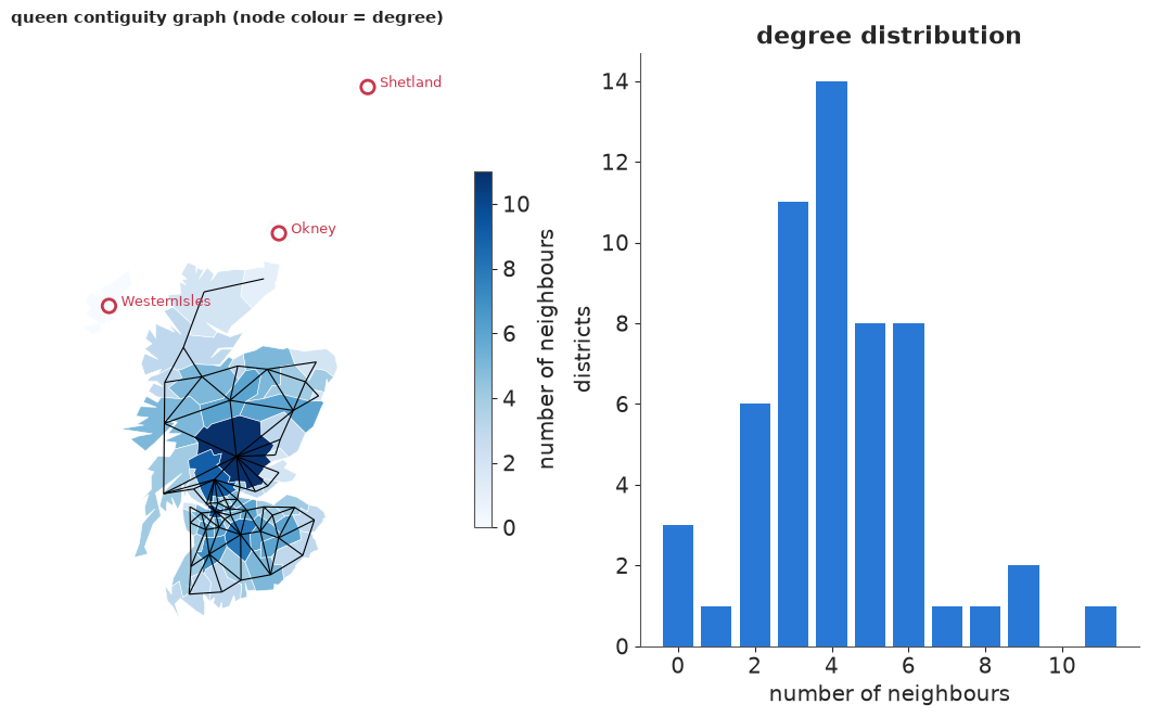
The mainland is one connected piece, but Orkney, Shetland and the Western Isles touch nothing: the graph has four components. (The GeoJSON spells Orkney "Okney"; we keep the source's spelling.) Degrees range from 0 to 11, and as we will see the degree matters: under an ICAR prior a district's variance depends on how many neighbours it has.
A published neighbour list, and why we do not simply trust it
The WinBUGS/GeoBUGS version of this dataset (reproduced in pymc-examples) ships a hand-edited neighbour list. Comparing it with our polygon graph is instructive.
data.describe("scotland_lip_adjacency")
bugs = data.load("scotland_lip_adjacency")
assert (bugs.CODENO.to_numpy() == lip.CODENO.to_numpy()).all()  # same districts, same order
W_bugs = np.zeros((N, N), dtype=int)
for i, nbrs in enumerate(bugs.ADJ):
    W_bugs[i, np.asarray(json.loads(nbrs)) - 1] = 1
print(f"published list: symmetric {bool((W_bugs == W_bugs.T).all())}, {W_bugs.sum() // 2} edges, "
      f"{connected_components(W_bugs, directed=False)[0]} component")
diff = W_bugs - W_queen
pd.DataFrame(
    [(names[i], names[j], "published only" if diff[i, j] > 0 else "polygons only",
      f"{np.linalg.norm(centroids[i] - centroids[j]) / 1000:.0f}") for i, j in zip(*np.nonzero(np.triu(diff)))],
    columns=["district", "district", "edge in", "centroid distance (km)"])
scotland_lip_adjacency: 56 districts: CANCER, CEXP, AFF and the published (hand-edited, islands linked) neighbour lists ADJ.
  source: Scottish lip cancer data with the WinBUGS GeoBUGS adjacency lists, via pymc-examples.
  url:    https://raw.githubusercontent.com/pymc-devs/pymc-examples/main/examples/data/scotland_lips_cancer.csv
published list: symmetric True, 132 edges, 1 component
| district | district | edge in | centroid distance (km) | |
|---|---|---|---|---|
| 0 | Skye-Lochalsh | WesternIsles | published only | 118 |
| 1 | Caithness | Okney | published only | 60 |
| 2 | Ross-Cromarty | WesternIsles | published only | 106 |
| 3 | Ross-Cromarty | Nairn | published only | 72 |
| 4 | Okney | Shetland | published only | 213 |
| 5 | Lochaber | WesternIsles | published only | 162 |
| 6 | WesternIsles | Sutherland | published only | 120 |
| 7 | NEFife | Dundee | published only | 22 |
| 8 | Roxburgh | Tweeddale | published only | 61 |
| 9 | Roxburgh | Annandale | polygons only | 47 |
| 10 | Argyll-Bute | Inverclyde | published only | 37 |
| 11 | Argyll-Bute | Cunninghame | published only | 49 |
| 12 | Dunfermline | Falkirk | published only | 25 |
| 13 | Nithsdale | Tweeddale | published only | 66 |
| 14 | Nithsdale | Annandale | polygons only | 38 |
| 15 | WestLothian | Tweeddale | polygons only | 31 |
| 16 | WestLothian | Annandale | published only | 86 |
| 17 | Stewartry | Kyle-Carrick | published only | 50 |
| 18 | Midlothian | Tweeddale | polygons only | 25 |
| 19 | Midlothian | Annandale | published only | 74 |
| 20 | Inverclyde | Dumbarton | published only | 23 |
| 21 | Dumbarton | Renfrew | published only | 32 |
| 22 | Clydebank | Renfrew | published only | 13 |
| 23 | Edinburgh | Tweeddale | polygons only | 31 |
| 24 | Edinburgh | Annandale | published only | 85 |
The published list has 132 edges to our 117. The differences fall into four groups:
- Islands linked by hand: Orkney to Caithness and Shetland, the Western Isles to four mainland districts. This is a modelling decision (ferries, shared fishing grounds), not geography.
- Estuary crossings: NE Fife - Dundee over the Tay, Dunfermline - Falkirk over the Forth, Argyll & Bute to Inverclyde and Cunninghame over the Clyde, plus three more pairs facing each other across the Clyde. Again defensible, again a decision.
- Near misses: Ross-Cromarty - Nairn (across the Moray Firth) and Stewartry - Kyle-Carrick, whose polygons do not touch on this simplified map.
- Tweeddale and Annandale look swapped. The polygons say Edinburgh, Midlothian and West Lothian border Tweeddale (correct: Peebles is 30 km south of Edinburgh), and that Roxburgh and Nithsdale border Annandale (correct: both lie along the Dumfriesshire border). The published list says the opposite for all five pairs. Somewhere between WinBUGS and this CSV the neighbour lists of the last two districts were attached to the wrong rows. It changes little here, since both districts have zero cases, but it is the kind of error that only a map reveals.
We build our own graph from the polygons and make the island decision explicitly.
Is there spatial structure at all? Moran's I
Before modelling, a classic descriptive check. Moran's I is the correlation between a value and the average of its neighbours, $I = \frac{N}{\sum_{ij} W_{ij}} \frac{\sum_{ij} W_{ij} z_i z_j}{\sum_i z_i^2}$ with $z$ centred; its reference distribution comes from shuffling the values over the map. We apply it to the log SMR (with 0.5 added to the counts so zeros are finite) on the mainland graph.
def morans_i(z, W):
    z = z - z.mean()
    return len(z) / W.sum() * (z @ W @ z) / (z @ z)


def moran_test(z, W, n_perm=4999):
    obs = morans_i(z, W)
    perm = np.array([morans_i(rng.permutation(z), W) for _ in range(n_perm)])
    return obs, (1 + (perm >= obs).sum()) / (n_perm + 1)


log_smr = np.log((y + 0.5) / E)
I_obs, p_val = moran_test(log_smr, W_queen)
print(f"Moran's I of log SMR = {I_obs:.2f} (permutation p = {p_val:.4f}; expectation under no pattern "
      f"{-1 / (N - 1):.2f})")
I_aff, p_aff = moran_test(aff, W_queen)
print(f"Moran's I of AFF      = {I_aff:.2f} (permutation p = {p_aff:.4f})")
Moran's I of log SMR = 0.50 (permutation p = 0.0002; expectation under no pattern -0.02)
Moran's I of AFF = 0.29 (permutation p = 0.0018)
Strong positive autocorrelation in both - neighbouring districts have similar SMRs and similar outdoor workforces. Moran's I tells us that there is structure. The models below tell us how much, where, and how much of it the covariate explains.
3 · Graph priors: ICAR, proper CAR and BYM2
All models share the Poisson likelihood with the expected count as offset,
$$y_i \sim \text{Poisson}(E_i \, r_i), \qquad \log r_i = \beta_0 + \beta_1 x_i + u_i,$$
with $x_i$ = (AFF$_i$ - mean) / 10, so $e^{\beta_1}$ is the relative risk per 10 percentage points of outdoor workforce. They differ only in the prior for the district effects $u$.
Graph Laplacian. With $D$ the diagonal matrix of degrees, $Q = D - W$ is the graph Laplacian, and $u^\top Q u = \sum_{i \sim j} (u_i - u_j)^2$ sums the squared differences over the edges. Every graph prior here penalises that sum.
- ICAR (intrinsic CAR, Besag 1974): $p(u) \propto \exp(-\frac{1}{2\sigma^2} u^\top Q u)$.
Equivalently, each $u_i$ given the rest is Normal around the mean of its
neighbours with variance $\sigma^2 / d_i$. $Q$ is singular - adding a constant to every
$u_i$ does not change a single difference - so the density is improper and must be pinned
down with a sum-to-zero constraint.
pm.ICARimposes it softly, as a tight Normal on $\sum_i u_i$. One constant per connected component is free, which is why islands matter. - Proper CAR: precision $\tau (D - \alpha W)$ with $0 < \alpha < 1$. Proper for $\alpha < 1$, and $\alpha \to 1$ recovers the ICAR.
- BYM (Besag, York & Mollié 1991): $u = \sigma_\phi \phi + \sigma_\theta \theta$, an ICAR component plus an iid one, because real maps have both smooth and area-specific variation.
- BYM2 (Riebler et al. 2016): $u = \sigma\left(\sqrt{\rho/s}\,\phi + \sqrt{1-\rho}\,\theta\right)$, the same sum re-parameterised by a total scale $\sigma$ and a mixing proportion $\rho \in (0, 1)$. The constant $s$ is the scaling factor of the graph, defined next.
Why the ICAR needs scaling: variances come from the graph
Under the constrained ICAR with $\sigma = 1$, the covariance of $\phi$ is the generalised inverse $Q^{+}$ of the Laplacian. Its diagonal - the marginal variances - is not constant: it depends on each area's position in the graph. The scaling factor is their geometric mean, $s = \exp\left(\frac{1}{N}\sum_i \log Q^{+}_{ii}\right)$; dividing $\phi$ by $\sqrt{s}$ gives a field whose typical marginal variance is 1, the same as the iid $\theta$. Only then do $\sigma$ and $\rho$ mean the same thing on every map.
To compute it we need a connected graph. We link each island to the district whose boundary is closest to it - a rule we can state and defend, where the published list made a judgement call per island.
def min_boundary_distance(i, j):
    return np.sqrt(((rings[i][:, None, :] - rings[j][None, :, :]) ** 2).sum(-1)).min()


W = W_queen.copy()
for i in islands:
    dist = np.array([np.inf if j == i else min_boundary_distance(i, j) for j in range(N)])
    j = int(dist.argmin())
    W[i, j] = W[j, i] = 1
    print(f"link {names[i]:>13s} -> {names[j]:<14s} ({dist[j] / 1000:.0f} km of sea)")
print(f"linked graph: {W.sum() // 2} edges, {connected_components(W, directed=False)[0]} component")


def scaling_factor(W):
    Q = np.diag(W.sum(1)) - W
    return np.exp(np.mean(np.log(np.diag(np.linalg.pinv(Q)))))


Q = np.diag(W.sum(1)) - W
Q_plus = np.linalg.pinv(Q)  # the generalised inverse = covariance of the constrained ICAR
s = scaling_factor(W)
print(f"scaling factor s = {s:.3f}; marginal variances range {np.diag(Q_plus).min():.2f} - {np.diag(Q_plus).max():.2f}")
link         Okney -> Caithness      (28 km of sea)
link      Shetland -> Okney          (192 km of sea)
link  WesternIsles -> Ross-Cromarty  (41 km of sea)
linked graph: 120 edges, 1 component
scaling factor s = 0.632; marginal variances range 0.23 - 4.60
Shetland's nearest district is Orkney, so the two northern islands form a chain hanging off Caithness; the graph is now connected. (The 192 km is an artefact: Shetland is drawn as a crude 7-point outline of its northern part only. The rule still picks Orkney.) The marginal variances of a unit ICAR on the linked graph span a factor of twenty. Where does that come from? The next figure plots them against the degree, and also asks the question that separates this notebook from E07: how does prior correlation relate to distance?
var_icar = np.diag(Q_plus)
corr_icar = Q_plus / np.sqrt(np.outer(var_icar, var_icar))
alpha_demo = 0.96
cov_car = np.linalg.inv(np.diag(W.sum(1)) - alpha_demo * W)
corr_car = cov_car / np.sqrt(np.outer(np.diag(cov_car), np.diag(cov_car)))
dist_km = np.linalg.norm(centroids[:, None] - centroids[None], axis=-1) / 1000
iu = np.triu_indices(N, 1)
is_edge = W[iu] == 1

fig, axes = plt.subplots(1, 3, figsize=(16, 4.8))
axes[0].scatter(W.sum(1) + rng.uniform(-0.15, 0.15, N), var_icar, color=BLUE, alpha=0.8)
for i in islands:
    axes[0].annotate(names[i], (W.sum(1)[i], var_icar[i]), xytext=(5, 0), textcoords="offset points", fontsize=8)
axes[0].axhline(s, color=ORANGE, ls="--", label=f"geometric mean s = {s:.2f}")
axes[0].set(xlabel="number of neighbours", ylabel=r"marginal variance $Q^{+}_{ii}$", yscale="log",
            title="ICAR variances depend on the graph")
axes[0].legend()
for ax, corr, label in [(axes[1], corr_icar, "ICAR"), (axes[2], corr_car, rf"proper CAR, $\alpha$ = {alpha_demo}")]:
    ax.scatter(dist_km[iu][~is_edge], corr[iu][~is_edge], s=6, color=GREY, alpha=0.5, label="not neighbours")
    ax.scatter(dist_km[iu][is_edge], corr[iu][is_edge], s=14, color=ORANGE, label="neighbours")
    ax.axhline(0, color="k", lw=0.6)
    ax.set(xlabel="distance between centroids (km)", ylabel="prior correlation", title=f"{label}: correlation vs distance")
    ax.legend(loc="upper right", fontsize=8)
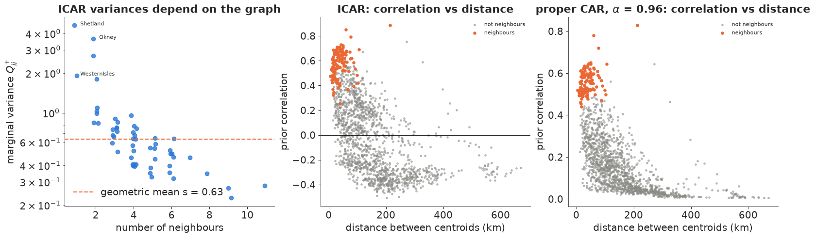
Three things to take from this figure.
- Poorly connected areas get large prior variances. A district with a single neighbour (the islands, peninsulas) is pinned down by one difference only; a central district with eight neighbours is held by eight. Under the ICAR the variance is a property of the graph, so the same $\sigma$ implies a different spread of risk on a different map - hence the scaling factor $s$ in BYM2.
- Correlation is not a function of distance. Under the ICAR, pairs 50 km apart have prior correlations anywhere from about 0.8 to below zero; two neighbours can be more or less correlated depending on what else they touch. A stationary GP (E07) makes correlation a smooth, decreasing function of distance by construction. An adjacency prior makes it a function of topology: a small urban district 5 km across and a Highland district 100 km across are treated alike if they have the same neighbours.
- The ICAR's correlations go negative at long range - a consequence of the sum-to-zero constraint: if the far north is above average, something else must be below. The proper CAR (here with $\alpha = 0.96$, near its posterior median below) has no constraint: its correlations decay towards zero instead, but scatter just as widely at a given distance.
Which is right? Neither in general. Adjacency is the natural choice when the areas are the unit at which things happen (health boards, school districts, policies) and when areas differ wildly in size; distance is natural for a continuous process observed at points (earthquakes, E07; soil, air quality). For areal data a GP on centroids ignores the areas' very different sizes, and an ICAR ignores the kilometres. An ICAR is also cheap: its precision matrix is sparse, with no $N \times N$ covariance to factorise.
Prior predictive, by hand
pm.ICAR has no random number generator (pm.sample_prior_predictive raises
NotImplementedError: Cannot sample from ICAR prior), so we draw from it ourselves: with
$Q^{+} = V \Lambda V^\top$, a constrained ICAR draw is $V \Lambda^{1/2} z$. Below: four draws
of the scaled ICAR field $\phi/\sqrt{s}$ and four of the iid field $\theta$, both on the scale
of log relative risk with $\sigma = 0.5$.
with pm.Model() as m_check, warnings.catch_warnings():
    warnings.simplefilter("ignore", UserWarning)  # a Numba "object mode" notice before the error
    pm.ICAR("phi", W=W)
    try:
        pm.sample_prior_predictive(draws=10, random_seed=RANDOM_SEED)
    except NotImplementedError as err:
        print("pm.sample_prior_predictive:", err)

lam, V = np.linalg.eigh(Q_plus)
lam = np.clip(lam, 0, None)  # the constant direction has eigenvalue 0 (numerically ~1e-16)


def draw_scaled_icar(n):
    return (V * np.sqrt(lam / s)) @ rng.standard_normal((N, n))


phi_draws = draw_scaled_icar(4).T
theta_draws = rng.standard_normal((4, N))
fig, axes = plt.subplots(2, 4, figsize=(16, 9))
for k in range(4):
    pc = draw_map(axes[0, k], 0.5 * phi_draws[k], cmap="RdBu_r", norm=RR_NORM, title=f"scaled ICAR draw {k + 1}")
    rr_colorbar_ticks(pc)
    pc = draw_map(axes[1, k], 0.5 * theta_draws[k], cmap="RdBu_r", norm=RR_NORM, title=f"iid draw {k + 1}")
    rr_colorbar_ticks(pc)
print(f"check: mean marginal variance of the scaled draws (geometric) = "
      f"{np.exp(np.mean(np.log(np.var(draw_scaled_icar(20000), axis=1)))):.2f}")
pm.sample_prior_predictive: Cannot sample from ICAR prior
check: mean marginal variance of the scaled draws (geometric) = 1.00
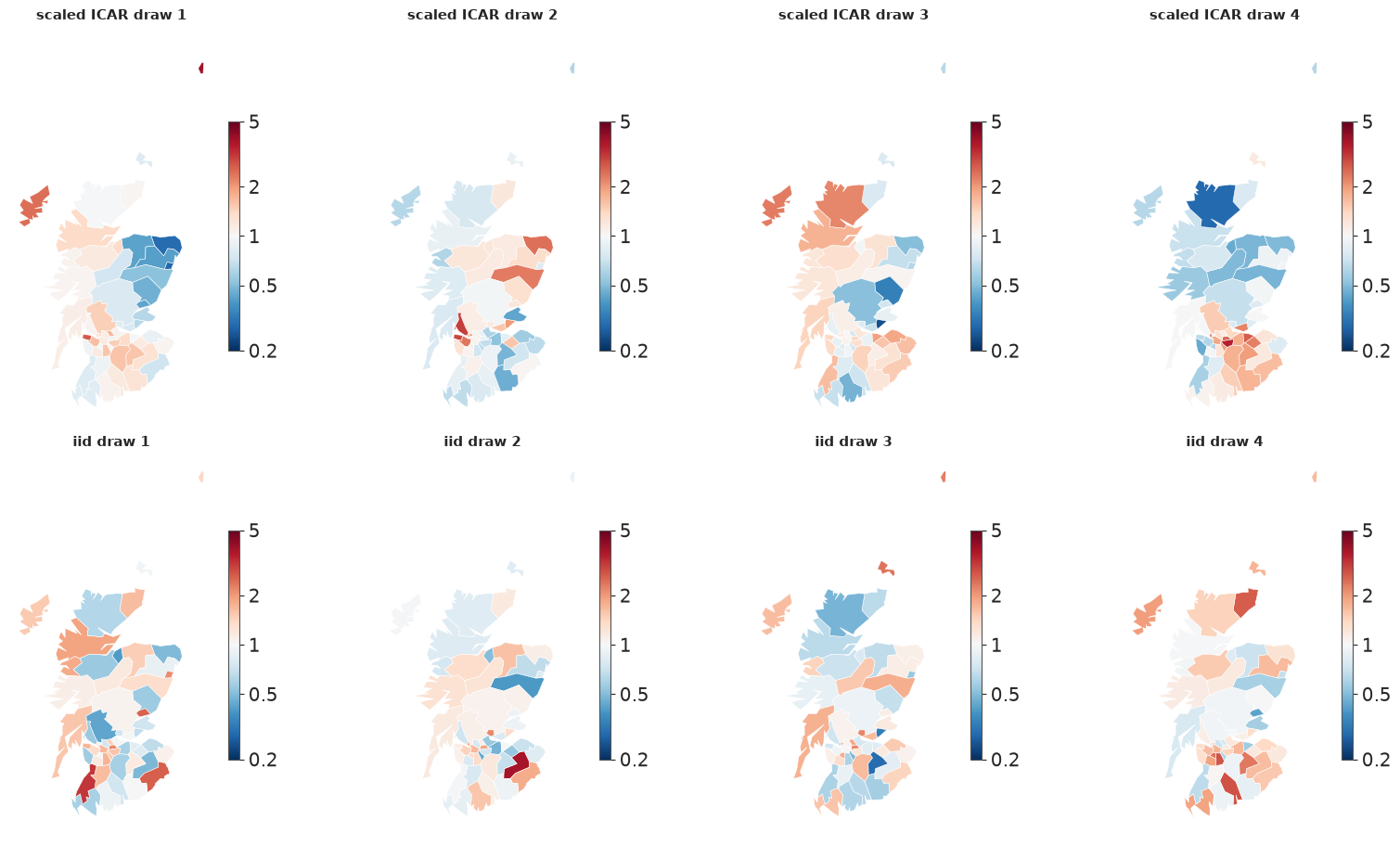
The ICAR draws are smooth patches spanning several districts, most variable at the poorly connected edges; the iid draws are confetti. Both have the same typical variance, so a HalfNormal(1) prior on $\sigma$ means the same thing for either. Its median, $\sigma \approx 0.67$, puts two thirds of the districts within a factor of about 2 of the baseline risk; its upper tail allows much more. Loose, but not absurd for a rare cancer in small populations.
4 · Fitting the ladder
Five models, each adding one idea: Poisson with the covariate only; iid district effects
(a Poisson-lognormal: extra-Poisson variation, no space); ICAR; proper CAR; BYM2. One
builder function makes them all, so that the only thing that changes is the prior on $u$.
The ICAR and BYM2 components are non-centred (pm.ICAR with unit scale, multiplied by
$\sigma$), the proper CAR is centred because pm.CAR takes the precision directly.
obs_idx restricts the likelihood to a subset of districts - we will need it for
cross-validation in section 8.
x = (aff - aff.mean()) / 10
coords = {"district": names}


def build(kind, W=W, obs_idx=None, scale=None):
    obs = np.arange(N) if obs_idx is None else np.asarray(obs_idx)
    with pm.Model(coords=coords) as model:
        b0 = pm.Normal("b0", 0.0, 1.0)
        b1 = pm.Normal("b1", 0.0, 1.0)
        if kind == "poisson":
            u = 0.0
        elif kind == "iid":
            sigma = pm.HalfNormal("sigma", 1.0)
            u = sigma * pm.Normal("theta", 0.0, 1.0, dims="district")
        elif kind == "icar":
            sigma = pm.HalfNormal("sigma", 1.0)
            u = sigma * pm.ICAR("phi", W=W, dims="district")
        elif kind == "car":
            sigma = pm.HalfNormal("sigma", 1.0)
            alpha = pm.Uniform("alpha", 0.0, 1.0)
            u = pm.CAR("phi", mu=np.zeros(N), W=W, alpha=alpha, tau=1 / sigma**2, dims="district")
        elif kind == "bym":  # the original, unscaled BYM
            sigma_phi = pm.HalfNormal("sigma_phi", 1.0)
            sigma_theta = pm.HalfNormal("sigma_theta", 1.0)
            phi = pm.ICAR("phi", W=W, dims="district")
            theta = pm.Normal("theta", 0.0, 1.0, dims="district")
            u = sigma_phi * phi + sigma_theta * theta
        elif kind == "bym2":
            s_ = scaling_factor(W) if scale is None else scale
            sigma = pm.HalfNormal("sigma", 1.0)
            rho = pm.Beta("rho", 1.0, 1.0)
            phi = pm.ICAR("phi", W=W, dims="district")
            theta = pm.Normal("theta", 0.0, 1.0, dims="district")
            u = sigma * (pm.math.sqrt(rho / s_) * phi + pm.math.sqrt(1 - rho) * theta)
        log_rr = pm.Deterministic("log_rr", b0 + b1 * x + u, dims="district")
        if obs_idx is None:
            pm.Poisson("y", mu=E * pm.math.exp(log_rr), observed=y, dims="district")
        else:
            pm.Poisson("y", mu=E[obs] * pm.math.exp(log_rr[obs]), observed=y[obs])
    return model


def fit(model, loglik=True, **kw):
    with model:
        idata = pm.sample(target_accept=0.9, random_seed=RANDOM_SEED, progressbar=False, **kw)
        if loglik:
            pm.compute_log_likelihood(idata, progressbar=False)
    return idata


def diagnostics(idata, var_names):
    summ = az.summary(idata, var_names=var_names, round_to=3)
    return summ.assign(divergences=int(idata.sample_stats["diverging"].sum()))[
        ["mean", "sd", "eti89_lb", "eti89_ub", "ess_bulk", "ess_tail", "r_hat", "divergences"]]


warnings.filterwarnings("ignore", message="Estimated shape parameter of Pareto")  # Pareto k: section 8
kinds = ["poisson", "iid", "icar", "car", "bym2"]
fits, loos = {}, {}
for kind in kinds:
    fits[kind] = fit(build(kind))
    loos[kind] = az.loo(fits[kind], pointwise=True)
    loos[kind].log_weights = None  # see AUTHORING.md: we only need elpd and Pareto k
print(f"warm-up steps: {fits['bym2'].posterior.attrs.get('tuning_steps')} (nutpie), 4 x 1000 draws each")

hyper = {"poisson": ["b0", "b1"], "iid": ["b0", "b1", "sigma"], "icar": ["b0", "b1", "sigma"],
         "car": ["b0", "b1", "sigma", "alpha"], "bym2": ["b0", "b1", "sigma", "rho"]}
pd.concat({k: diagnostics(fits[k], hyper[k]) for k in kinds})
warm-up steps: 400 (nutpie), 4 x 1000 draws each
| mean | sd | eti89_lb | eti89_ub | ess_bulk | ess_tail | r_hat | divergences | ||
|---|---|---|---|---|---|---|---|---|---|
| poisson | b0 | 0.095 | 0.043 | 0.025 | 0.163 | 4294.844 | 2745.083 | 1.002 | 0 |
| b1 | 0.736 | 0.060 | 0.642 | 0.830 | 3585.365 | 2361.048 | 1.003 | 0 | |
| iid | b0 | 0.097 | 0.097 | -0.059 | 0.247 | 1569.929 | 2020.427 | 1.001 | 0 |
| b1 | 0.670 | 0.146 | 0.433 | 0.905 | 1457.777 | 1804.148 | 1.001 | 0 | |
| sigma | 0.623 | 0.089 | 0.493 | 0.775 | 1085.707 | 1416.082 | 1.002 | 0 | |
| icar | b0 | 0.099 | 0.051 | 0.018 | 0.181 | 4447.485 | 3581.224 | 1.001 | 0 |
| b1 | 0.374 | 0.124 | 0.173 | 0.567 | 1950.381 | 2420.455 | 1.003 | 0 | |
| sigma | 0.673 | 0.119 | 0.502 | 0.878 | 634.068 | 929.774 | 1.005 | 0 | |
| car | b0 | 0.020 | 0.297 | -0.451 | 0.503 | 112.668 | 124.298 | 1.033 | 0 |
| b1 | 0.398 | 0.131 | 0.185 | 0.599 | 1375.512 | 2004.336 | 1.003 | 0 | |
| sigma | 0.728 | 0.134 | 0.535 | 0.958 | 1018.241 | 1330.788 | 1.001 | 0 | |
| alpha | 0.958 | 0.044 | 0.879 | 0.997 | 669.242 | 829.070 | 1.006 | 0 | |
| bym2 | b0 | 0.101 | 0.059 | 0.006 | 0.193 | 4483.028 | 3399.840 | 1.000 | 0 |
| b1 | 0.404 | 0.129 | 0.196 | 0.612 | 3177.886 | 3166.098 | 1.001 | 0 | |
| sigma | 0.515 | 0.084 | 0.393 | 0.658 | 1247.921 | 1716.033 | 1.003 | 0 | |
| rho | 0.819 | 0.152 | 0.523 | 0.988 | 660.891 | 1110.797 | 1.002 | 0 |
Everything samples in seconds with no divergences and $\hat r \le 1.01$, except the proper CAR, whose intercept has a bulk ESS of about 110 and $\hat r \approx 1.03$, with $\alpha$ pushed against 1. That is failure number two; we come back to it in section 5. The headline numbers already tell a story:
- $\beta_1$, the AFF effect, drops from about 0.67 (iid) to about 0.4 (all spatial models). Section 7 is about why.
- The spatial models agree with each other closely on $\beta_0$, $\beta_1$ and the size of the district effects.
Posterior predictive check: is the leftover variation spatial?
A random-effects model always fits the counts (each district has its own parameter), so a count-level PPC says little. The sharper question is whether the iid model's residual effects $\theta_i$ still carry spatial structure - if so, the model's assumption of independent districts is wrong. We compute Moran's I of the posterior-mean effects, and for the BYM2 of its unstructured part $\theta$ only. We also check plain overdispersion for the Poisson-only model: the share of districts whose count falls outside the central 90% posterior predictive interval.
def post_mean(idata, var):
    return idata.posterior[var].mean(("chain", "draw")).to_numpy()


for label, idata, var in [("iid model, theta", fits["iid"], "theta"), ("BYM2, unstructured theta", fits["bym2"], "theta"),
                          ("BYM2, structured phi", fits["bym2"], "phi")]:
    I, p = moran_test(post_mean(idata, var), W, n_perm=1999)
    print(f"Moran's I of {label:<26s}: {I:5.2f} (permutation p = {p:.3f})")

for kind in ["poisson", "iid", "bym2"]:
    with build(kind):
        pp = pm.sample_posterior_predictive(fits[kind], random_seed=RANDOM_SEED, progressbar=False)
    lo, hi = np.quantile(pp.posterior_predictive["y"].to_numpy().reshape(-1, N), [0.05, 0.95], axis=0)
    print(f"{kind:>8s}: {np.mean((y < lo) | (y > hi)):.0%} of districts outside their 90% predictive interval")
Moran's I of iid model, theta          :  0.35 (permutation p = 0.001)
Moran's I of BYM2, unstructured theta  : -0.08 (permutation p = 0.739)
Moran's I of BYM2, structured phi      :  0.77 (permutation p = 0.001)
poisson: 39% of districts outside their 90% predictive interval
iid: 0% of districts outside their 90% predictive interval
bym2: 0% of districts outside their 90% predictive interval
The Poisson-only model leaves 39% of the districts outside their 90% intervals: there is far more variation between districts than AFF explains. The two random-effects models leave none outside - which says only that a model with one parameter per district can fit 56 counts, not that it is right. Moran's I is more informative: the iid model's residual effects are still clearly autocorrelated (0.35, against 0.50 for the raw log SMR). Independent effects soak up the overdispersion but leave the map's structure unexplained. In the BYM2 the structured part $\phi$ takes the spatial pattern ($I = 0.77$), and the unstructured remainder shows none ($I = -0.08$).
5 · Three failures and their fixes
Failure 1: islands
What if we had kept the raw polygon graph, with its three isolated islands?
Loudly: the BYM2 scaling factor does not exist. An isolated node's row of $Q$ is all zeros, so its generalised-inverse variance is 0 (here $-0$ from rounding), the log is $-\infty$ or NaN, and so is $s$. The model's log-density at the starting point is $-\infty$, so sampling fails before it starts.
with np.errstate(divide="ignore", invalid="ignore"):
    s_raw = scaling_factor(W_queen)
print(f"diag of pinv(Q) for the islands: {np.diag(np.linalg.pinv(np.diag(degree) - W_queen))[islands].round(12)}")
print(f"scaling factor on the raw graph: {s_raw}")
with np.errstate(divide="ignore", invalid="ignore"):
    m_bad = build("bym2", W=W_queen, scale=s_raw)
print("log-density at the initial point:", m_bad.point_logps())
diag of pinv(Q) for the islands: [-0. -0.  0.]
scaling factor on the raw graph: nan
log-density at the initial point: {'b0': np.float64(-0.92), 'b1': np.float64(-0.92), 'sigma': np.float64(-0.73), 'rho': np.float64(-1.39), 'phi': np.float64(1.96), 'theta': np.float64(-51.46), 'y': np.float64(-inf)}
Quietly: the ICAR samples fine and gives the islands no prior at all. Look at the ICAR density again: an isolated $\phi_i$ appears in no difference $(\phi_i - \phi_j)^2$, so the only thing that touches it is the global soft sum-to-zero term. Its prior is flat. The model runs without a warning, and the islands are estimated from their own counts alone - no pooling - while the global constraint now also has to absorb the level of three separate components.
fit_islands = fit(build("icar", W=W_queen), loglik=False)
print(diagnostics(fit_islands, ["b0", "b1", "sigma"]))


def rr_summary(idata, idx):
    rr = np.exp(idata.posterior["log_rr"].isel(district=idx).to_numpy().reshape(-1, len(idx)))
    return [f"{m:.2f} [{lo:.2f}, {hi:.2f}]" for m, lo, hi in zip(np.median(rr, 0), *np.quantile(rr, [0.05, 0.95], 0))]


pd.DataFrame({"y": y[islands], "E": E[islands], "SMR": lip.SMR.to_numpy()[islands].round(2),
              "iid": rr_summary(fits["iid"], islands),
              "ICAR, islands isolated": rr_summary(fit_islands, islands),
              "ICAR, islands linked": rr_summary(fits["icar"], islands)},
             index=names[islands]).rename_axis("relative risk: median [90%]")
        mean     sd  eti89_lb  eti89_ub  ess_bulk  ess_tail  r_hat  \
b0     0.102  0.051     0.019     0.183  4973.410  3178.462  1.001
b1     0.422  0.127     0.219     0.624  1908.444  2534.376  1.000
sigma  0.639  0.113     0.475     0.831   613.572   968.079  1.005

       divergences
b0               0
b1               0
sigma 0 | y | E | SMR | iid | ICAR, islands isolated | ICAR, islands linked | |
|---|---|---|---|---|---|---|
| relative risk: median [90%] | ||||||
| Okney | 8 | 2.4 | 3.33 | 3.18 [1.84, 5.28] | 3.18 [1.66, 5.36] | 3.84 [2.31, 5.89] |
| Shetland | 7 | 2.3 | 3.04 | 2.10 [1.09, 3.71] | 2.91 [1.42, 5.26] | 2.61 [1.39, 4.49] |
| WesternIsles | 13 | 4.4 | 2.95 | 2.36 [1.44, 3.63] | 2.86 [1.75, 4.41] | 2.86 [1.82, 4.31] |
Compare the columns. With the islands isolated, their relative risks sit just below the raw SMR with wide intervals: they are practically unpooled fixed effects that happen to share a sampler with a spatial model. The iid model shrinks them towards the national regression line - Shetland, with a low AFF, the most (3.0 to 2.1). Linked, they are shrunk towards their neighbours instead: Orkney moves up (its neighbour Caithness has an SMR of 3.6), Shetland moves towards Orkney. Neither answer is automatically right - whether Shetland should borrow strength from Orkney is a substantive question - but the isolated version is not a decision anyone made; it is a side effect.
Fixes, in order of preference:
- Decide on links for islands explicitly (ferry routes, nearest district, as here) and say so.
- Keep the components separate and do it properly (Freni-Sterrantino, Ventrucci & Rue
2018): a sum-to-zero constraint per component, a scaling factor per component, and
for singletons only the iid part.
pm.ICARapplies one global constraint, so this needs a custom density (try it at the end).
Failure 2: the proper CAR's $\alpha$ sits at the boundary
The proper CAR looked attractive: a proper density, no constraint, no scaling. But its posterior for $\alpha$ is piled against 1, and the intercept mixes badly.
alpha_draws = fits["car"].posterior["alpha"].to_numpy().ravel()
print(f"alpha: median {np.median(alpha_draws):.3f}, 5% quantile {np.quantile(alpha_draws, 0.05):.3f}")
print(f"b0 ESS bulk: CAR {float(az.ess(fits['car'], var_names=['b0'])['b0']):.0f}, "
      f"BYM2 {float(az.ess(fits['bym2'], var_names=['b0'])['b0']):.0f}")

alphas = np.linspace(0.0, 0.999, 60)
neigh_corr = []
for a in alphas:
    cov = np.linalg.inv(np.diag(W.sum(1)) - a * W)
    c = cov / np.sqrt(np.outer(np.diag(cov), np.diag(cov)))
    neigh_corr.append(c[iu][is_edge].mean())

fig, axes = plt.subplots(1, 3, figsize=(16, 4.5))
axes[0].hist(alpha_draws, bins=60, color=BLUE, density=True)
axes[0].set(xlabel=r"$\alpha$", title=r"posterior of $\alpha$ (prior: uniform)")
axes[1].plot(alphas, neigh_corr, color=ORANGE, lw=2)
axes[1].set(xlabel=r"$\alpha$", ylabel="mean neighbour correlation",
            title=r"what $\alpha$ means on this graph")
axes[1].axvspan(np.quantile(alpha_draws, 0.05), 1, color=BLUE, alpha=0.15, label="posterior 90% upper region")
axes[1].legend(fontsize=8)
axes[2].scatter(alpha_draws, fits["car"].posterior["b0"].to_numpy().ravel(), s=3, alpha=0.3, color=BLUE)
axes[2].set(xlabel=r"$\alpha$", ylabel=r"$\beta_0$", title=r"as $\alpha \to 1$ the intercept loses its anchor");
alpha: median 0.972, 5% quantile 0.874
b0 ESS bulk: CAR 113, BYM2 4483
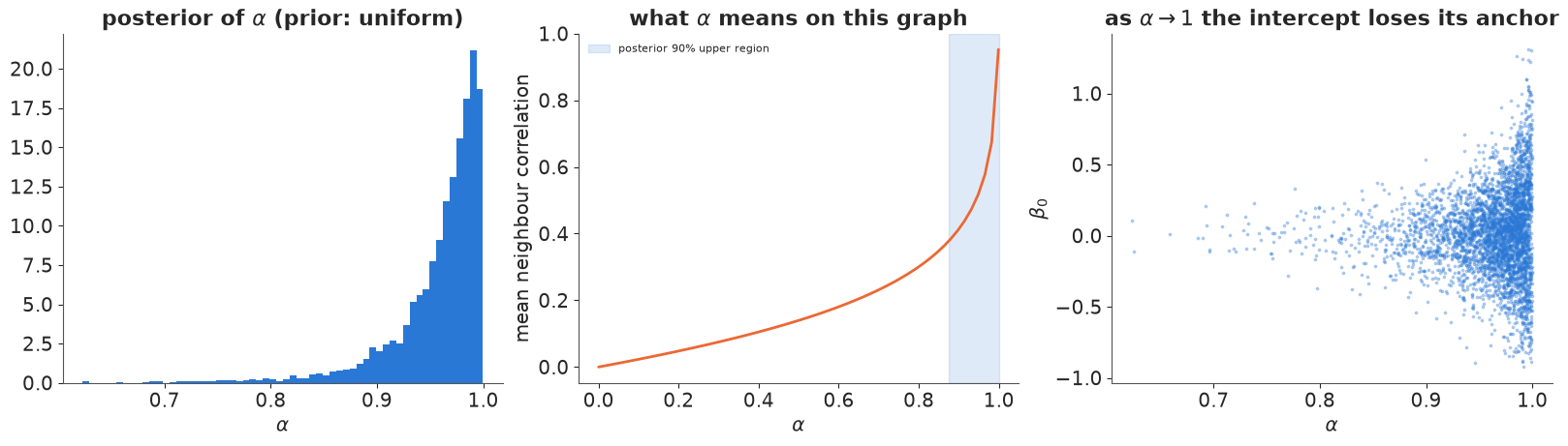
Two reasons, both structural rather than numerical:
- $\alpha$ is not a correlation. On this graph the average prior correlation between neighbours is still below 0.3 at $\alpha = 0.8$ and only climbs steeply in the last few hundredths before 1. A uniform prior on $\alpha$ therefore puts most of its mass on weak spatial dependence, and data with real spatial structure have to push $\alpha$ into the corner (Wall 2004 documents this for US states).
- At $\alpha \to 1$ the constant direction becomes (almost) free. The proper CAR's precision approaches the singular Laplacian, so the mean level of $\phi$ and the intercept $\beta_0$ trade off, as the right panel shows. That is where the low ESS of $\beta_0$ comes from.
Fix: use the ICAR (the $\alpha = 1$ limit, with the constraint that removes the free direction) and, when the data may be less smooth, mix it with iid noise - which is BYM2. The proper CAR still has its place (it is a valid model on graphs where you want weak dependence and a proper prior), but $\alpha$ should not be read as "how spatial".
Failure 3: the unscaled BYM - two scales that do not mean the same thing
The original BYM puts separate priors on $\sigma_\phi$ (ICAR) and $\sigma_\theta$ (iid). It samples fine here, but its parameters are hard to read and its priors are silently unequal.
fit_bym = fit(build("bym"), loglik=False)
print(diagnostics(fit_bym, ["b0", "b1", "sigma_phi", "sigma_theta"]))
post_bym = az.extract(fit_bym, var_names=["sigma_phi", "sigma_theta"])
sp, st = post_bym["sigma_phi"].to_numpy(), post_bym["sigma_theta"].to_numpy()
print(f"corr(sigma_phi, sigma_theta) = {np.corrcoef(sp, st)[0, 1]:.2f}")
naive = sp**2 / (sp**2 + st**2)
marginal = s * sp**2 / (s * sp**2 + st**2)
rho_bym2 = fits["bym2"].posterior["rho"].to_numpy().ravel()
print(f"'spatial share' sigma_phi^2 / (sigma_phi^2 + sigma_theta^2): median {np.median(naive):.2f}")
print(f"same with the ICAR's actual marginal variance s * sigma_phi^2: median {np.median(marginal):.2f}")
print(f"BYM2 rho: median {np.median(rho_bym2):.2f}")
sp0, st0 = np.abs(rng.standard_normal((2, 100_000)))  # the BYM prior: two HalfNormal(1) scales
share0 = s * sp0**2 / (s * sp0**2 + st0**2)
print(f"prior on the spatial share implied by the BYM priors: median {np.median(share0):.2f}, "
      f"P(share > 0.5) = {np.mean(share0 > 0.5):.2f}   (BYM2: 0.50 and 0.50 by construction)")
              mean     sd  eti89_lb  eti89_ub  ess_bulk  ess_tail  r_hat  \
b0           0.100  0.056     0.010     0.187  4623.618  3488.097  1.003
b1           0.390  0.133     0.179     0.597  3217.581  3100.696  1.001
sigma_phi    0.633  0.128     0.441     0.844   770.578   872.236  1.008
sigma_theta  0.149  0.104     0.016     0.340   708.396   895.144  1.009

             divergences
b0                     0
b1                     0
sigma_phi              0
sigma_theta            0
corr(sigma_phi, sigma_theta) = -0.33
'spatial share' sigma_phi^2 / (sigma_phi^2 + sigma_theta^2): median 0.96
same with the ICAR's actual marginal variance s * sigma_phi^2: median 0.94
BYM2 rho: median 0.86
prior on the spatial share implied by the BYM priors: median 0.39, P(share > 0.5) = 0.43   (BYM2: 0.50 and 0.50 by construction)
$\sigma_\phi$ is a conditional standard deviation (of $\phi_i$ given its neighbours, for one neighbour), while $\sigma_\theta$ is a marginal one. On this graph a unit ICAR has typical marginal variance $s \approx 0.63$, so the same HalfNormal(1) prior on the two scales quietly favours the iid part (the implied prior on the spatial share has its median below 0.5) - and on a different map, with another $s$, the tilt would be different. The two scales are also negatively correlated in the posterior: the data constrain their total better than their split.
The posterior share differs between the two parameterisations - about 0.94 for BYM, 0.86 for BYM2's $\rho$ - and neither is "the" answer: the data say "mostly spatial", and the rest is prior, which also enters through the priors on the total scale. With BYM that prior is implicit and graph-dependent; with BYM2 you set it directly on the quantity you report, and the same prior means the same thing on every map.
6 · BYM2: how spatial is the risk?
post2 = az.extract(fits["bym2"], var_names=["sigma", "rho"])
fig, axes = plt.subplots(1, 2, figsize=(12, 4))
axes[0].hist(post2["rho"].to_numpy(), bins=50, density=True, color=BLUE, alpha=0.8, label="posterior")
axes[0].axhline(1, color=GREY, ls="--", label="prior Beta(1, 1)")
axes[0].set(xlabel=r"$\rho$ = spatial share of the district-effect variance", title=r"BYM2 mixing parameter")
axes[0].legend()
axes[1].hist(post2["sigma"].to_numpy(), bins=50, density=True, color=ORANGE, alpha=0.8, label="posterior")
sig_grid = np.linspace(0, 1.5, 200)
axes[1].plot(sig_grid, stats.halfnorm(scale=1).pdf(sig_grid), color=GREY, ls="--", label="prior HalfNormal(1)")
axes[1].set(xlabel=r"$\sigma$ (total sd of log relative risk)", title="BYM2 total scale")
axes[1].legend()
print(f"rho: median {np.median(post2['rho']):.2f}, 90% interval "
      f"[{np.quantile(post2['rho'], 0.05):.2f}, {np.quantile(post2['rho'], 0.95):.2f}]; P(rho > 0.5) = "
      f"{np.mean(post2['rho'].to_numpy() > 0.5):.2f}")
rho: median 0.86, 90% interval [0.52, 0.99]; P(rho > 0.5) = 0.96
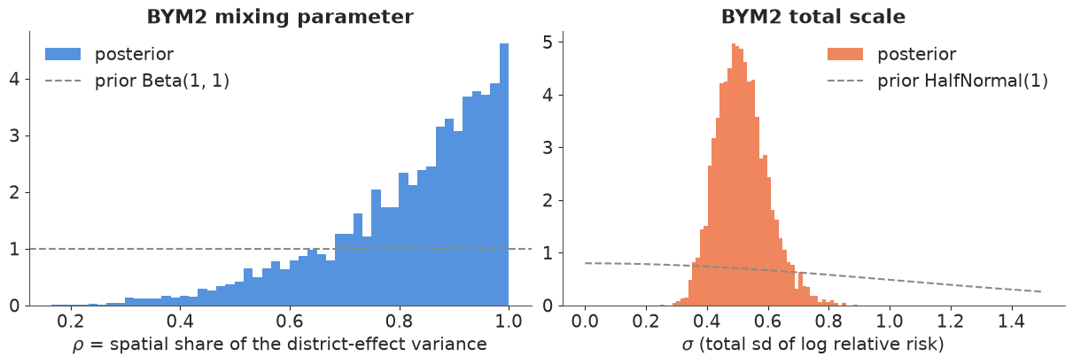
Most of the district-to-district variation beyond AFF is spatially structured: $\rho$'s posterior is concentrated well above 0.5, with a long tail down that reflects how little 56 districts can say about a variance split. In epidemiological terms: after adjusting for outdoor work, a district's lip-cancer risk is better predicted by its neighbours' risk than by an independent district-level quirk - pointing to further unmeasured, geographically smooth risk factors (sun exposure that the share of outdoor workers does not capture, for instance).
7 · Maps: what to report
The raw SMR map is the wrong thing to publish: its most extreme colours belong to the smallest districts. The BYM2 posterior gives two better maps: the smoothed relative risk (posterior median of $r_i$), and the exceedance probability $P(r_i > 1 \mid y)$ - the answer to "is this district's risk really above the national level?"
rr_draws = np.exp(fits["bym2"].posterior["log_rr"].to_numpy().reshape(-1, N))
rr_med = np.median(rr_draws, 0)
p_exceed = (rr_draws > 1).mean(0)

fig, axes = plt.subplots(1, 3, figsize=(16, 6.5))
pc = draw_map(axes[0], np.log(np.clip(lip.SMR, 0.2, None)), cmap="RdBu_r", norm=RR_NORM, title="raw SMR", cbar_label="SMR")
rr_colorbar_ticks(pc)
pc = draw_map(axes[1], np.log(rr_med), cmap="RdBu_r", norm=RR_NORM, title="BYM2 smoothed relative risk (median)",
              cbar_label="relative risk")
rr_colorbar_ticks(pc)
draw_map(axes[2], p_exceed, cmap="PuOr_r", norm=TwoSlopeNorm(vcenter=0.5, vmin=0, vmax=1),
         title="exceedance probability P(RR > 1)", cbar_label="probability")
hot = p_exceed > 0.95
axes[2].scatter(*centroids[hot].T, marker="+", color="k", s=40)
print(f"{hot.sum()} districts with P(RR > 1) > 0.95, {(p_exceed < 0.05).sum()} with P(RR > 1) < 0.05")
19 districts with P(RR > 1) > 0.95, 14 with P(RR > 1) < 0.05
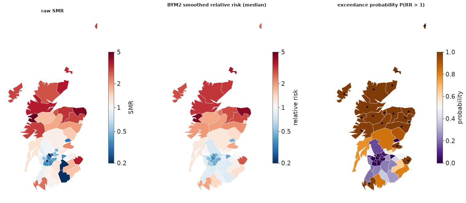
The smoothed map keeps the north-west / central-belt contrast but tones down the extremes, and the zero-count districts in the south-east are no longer painted as the healthiest in Scotland. The exceedance map (crosses: $P > 0.95$) is what a public-health reader should see: it separates "high and certain" from "high but based on nine cases".
Shrinkage: who moved, and why
fig, axes = plt.subplots(1, 2, figsize=(15, 6))
rr_iid = np.median(np.exp(fits["iid"].posterior["log_rr"].to_numpy().reshape(-1, N)), 0)
smr_plot = np.clip(lip.SMR.to_numpy(), 0.15, None)
ax = axes[0]
for i in range(N):
    ax.plot([0, 1], [smr_plot[i], rr_med[i]], color=GREY, lw=0.8, alpha=0.7)
ax.scatter(np.zeros(N), smr_plot, s=8 * np.sqrt(E) * 3, color=ORANGE, alpha=0.7, label="raw SMR (size ~ sqrt E)")
ax.scatter(np.ones(N), rr_med, s=8 * np.sqrt(E) * 3, color=BLUE, alpha=0.7, label="BYM2 median RR")
ax.set(yscale="log", xticks=[0, 1], xticklabels=["raw SMR", "BYM2"], ylabel="relative risk (log scale)",
       title="shrinkage: small districts move most")
ax.legend(loc="upper center", fontsize=8)
ax = axes[1]
nb_mean = np.array([np.mean(np.log(smr_plot[W[i] == 1])) for i in range(N)])
ax.scatter(np.log(rr_iid) - np.log(smr_plot), np.log(rr_med) - np.log(smr_plot), c=nb_mean - np.log(smr_plot),
           cmap="RdBu_r", s=8 * np.sqrt(E) * 3, norm=TwoSlopeNorm(0), edgecolor="k", lw=0.3)
lim = [-1.2, 1.9]
ax.plot(lim, lim, color="k", lw=0.8, ls="--")
ax.set(xlim=lim, ylim=lim, xlabel="log shift from SMR, iid model", ylabel="log shift from SMR, BYM2",
       title="colour: neighbours' mean log SMR minus own (red = higher)")
for i in np.argsort(-np.abs(np.log(rr_med) - np.log(rr_iid)))[:5]:
    ax.annotate(names[i], (np.log(rr_iid[i]) - np.log(smr_plot[i]), np.log(rr_med[i]) - np.log(smr_plot[i])),
                fontsize=8, xytext=(4, 4), textcoords="offset points");
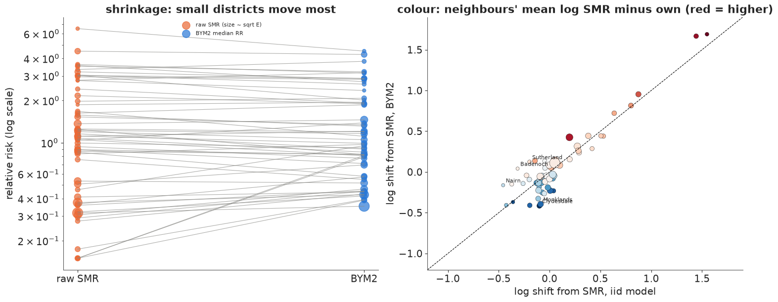
(Zero counts are drawn at SMR 0.15: they are the two points at the top right.) Left: every district is pulled towards a consensus, and the small ones (small dots) move the most - the usual hierarchical-model shrinkage (E02). Right: where they are pulled differs between the models. The iid model pulls every district towards the same national regression line; BYM2 pulls it towards its neighbours. Points off the diagonal are districts where the two disagree, and the colour shows why: districts whose neighbours have higher SMRs (red) are pulled up more by BYM2 than by the iid model, and vice versa.
8 · Model comparison: LOO, and why to distrust it here
comparison = az.compare(loos, round_to=1)
print(comparison[["elpd", "elpd_diff", "dse", "p", "weight"]])
pd.DataFrame({k: [(v.pareto_k.values > 0.7).sum(), v.pareto_k.values.max().round(2)] for k, v in loos.items()},
             index=["Pareto k > 0.7", "max k"]).T
          elpd  elpd_diff   dse     p  weight
icar    -151.9        0.0   0.0  24.5     1.0
bym2    -152.7       -0.8   0.7  25.8     0.0
car     -152.8       -0.9   0.8  25.7     0.0
iid     -163.6      -11.7   3.1  37.1     0.0
poisson -230.7      -78.8  20.1  11.4     0.0
| Pareto k > 0.7 | max k | |
|---|---|---|
| poisson | 0.0 | 0.69 |
| iid | 28.0 | 1.24 |
| icar | 17.0 | 0.98 |
| car | 17.0 | 1.02 |
| bym2 | 24.0 | 1.03 |
LOO ranks the three graph models within one elpd of each other, all 11-12 above iid (3-4 standard errors), which is itself far above the Poisson-only model. But look at the Pareto $k$: between 17 and 28 of the 56 districts have $k > 0.7$ in every random-effects model. That is structural, not a bug: each district's count is the main source of information about its own effect $u_i$, so deleting it changes the posterior too much for importance sampling to recover. The ranking is plausible, but these elpd values should not be quoted as precise.
The honest check is to actually refit without the held-out districts. Leaving a district out is also exactly the prediction problem an areal model is for: what is the risk in a district we have no data for? The iid model can only answer with the regression line; the graph models answer with the neighbours. We run 8-fold cross-validation (7 districts per fold, the same folds for every model) and score the held-out counts with the exact log predictive density. That is 32 fits of a few seconds each.
folds = np.array_split(rng.permutation(N), 8)
cv_models = ["iid", "icar", "car", "bym2"]
elpd_cv = {k: np.zeros(N) for k in cv_models}
for kind in cv_models:
    for test in folds:
        train = np.setdiff1d(np.arange(N), test)
        idata_k = fit(build(kind, obs_idx=train), loglik=False)
        mu = E[test] * np.exp(idata_k.posterior["log_rr"].isel(district=test).to_numpy().reshape(-1, len(test)))
        elpd_cv[kind][test] = logsumexp(stats.poisson.logpmf(y[test], mu), axis=0) - np.log(mu.shape[0])
        del idata_k
cv = pd.DataFrame({"elpd (8-fold)": {k: v.sum() for k, v in elpd_cv.items()},
                   "se": {k: np.sqrt(N) * v.std() for k, v in elpd_cv.items()}})
cv["diff vs BYM2"] = cv["elpd (8-fold)"] - cv.loc["bym2", "elpd (8-fold)"]
cv["se of diff"] = {k: np.sqrt(N) * (elpd_cv[k] - elpd_cv["bym2"]).std() for k in cv_models}
cv.round(1)
| elpd (8-fold) | se | diff vs BYM2 | se of diff | |
|---|---|---|---|---|
| iid | -175.1 | 6.4 | -17.8 | 3.5 |
| icar | -156.4 | 5.8 | 1.0 | 0.6 |
| car | -157.1 | 5.7 | 0.3 | 0.7 |
| bym2 | -157.4 | 5.7 | 0.0 | 0.0 |
Cross-validation that genuinely withholds districts gives lower elpd than PSIS-LOO for every model (8-fold holds out 7 districts at a time, and PSIS was optimistic where $k$ was high), but it confirms the ordering: predicting a district from its neighbours beats predicting it from the covariate alone by about 18 elpd, five standard errors, while the three graph models are close: the pure ICAR scores about 1 higher than BYM2 (the paired difference has a standard error of about 0.6), consistent with $\rho$ near 1 - when almost all the variation is spatial, the iid part of BYM2 mostly adds noise to the prediction of a held-out district. That is about 1 nat summed over 56 districts, a small difference; with this much data the choice between ICAR, proper CAR and BYM2 is better made on interpretability and behaviour (BYM2: an interpretable $\rho$, priors that transfer between maps, no boundary problem, and safety when the data are not so spatial).
9 · The covariate: spatial confounding
The AFF effect fell from about 0.67 to about 0.4 when the spatial term went in. Which is the effect of outdoor work?
b1_tab = pd.DataFrame({k: np.quantile(fits[k].posterior["b1"].to_numpy().ravel(), [0.05, 0.5, 0.95]) for k in kinds},
                      index=["5%", "median", "95%"]).T
b1_tab["RR per +10 points (median)"] = np.exp(b1_tab["median"])
print(b1_tab.round(2))

pb = az.extract(fits["bym2"], var_names=["log_rr", "b0", "b1"])
u_draws = pb["log_rr"].to_numpy() - pb["b0"].to_numpy() - np.outer(x, pb["b1"].to_numpy())  # (district, sample)
u_med = np.median(u_draws, 1)
fig, axes = plt.subplots(1, 3, figsize=(16, 6))
fig_x = np.arange(len(kinds))
axes[0].errorbar(b1_tab["median"], fig_x, xerr=[b1_tab["median"] - b1_tab["5%"], b1_tab["95%"] - b1_tab["median"]],
                 fmt="o", color=BLUE, capsize=3)
axes[0].set(yticks=fig_x, yticklabels=kinds, xlabel=r"$\beta_1$ (log RR per 10 points of AFF), 90% interval",
            title="the AFF effect depends on the random effects")
axes[0].axvline(0, color=GREY, lw=0.8)
draw_map(axes[1], x * 10, cmap="YlGn", title="AFF (centred, percentage points)", cbar_label="points")
pc = draw_map(axes[2], u_med, cmap="RdBu_r", norm=RR_NORM, title="BYM2 district effect $u_i$ (median)", cbar_label="exp(u)")
rr_colorbar_ticks(pc)
print(f"correlation between AFF and the BYM2 district effect: {np.corrcoef(x, u_med)[0, 1]:.2f}")
           5%  median   95%  RR per +10 points (median)
poisson  0.64    0.74  0.83                        2.09
iid      0.43    0.67  0.91                        1.96
icar     0.17    0.38  0.57                        1.46
car      0.18    0.40  0.60                        1.49
bym2     0.19    0.41  0.62                        1.50
correlation between AFF and the BYM2 district effect: 0.35
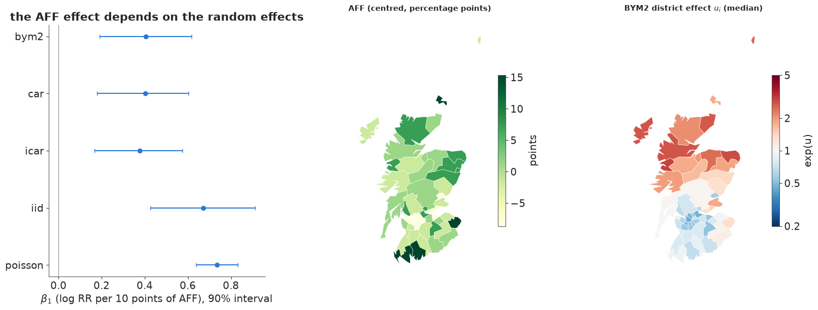
AFF is itself spatially patterned (Moran's I 0.29 in section 2): high in the north and the rural south-west, low in the central belt, much like the risk. Part of it therefore lies in the space that the spatial effect can also represent, and the estimated district effect is still correlated with AFF (0.35). The model cannot distinguish "outdoor work raises risk" from "the north has higher risk for reasons we have not measured, and happens to farm and fish", so it splits the credit: the AFF coefficient drops by about 40% (from a relative risk of about 1.96 to about 1.5 per 10 points). This is spatial confounding (Clayton, Bernardinelli & Montomoli 1993; Hodges & Reich 2010).
Neither number is "the" effect:
- The iid estimate assumes nothing else varies smoothly across Scotland. If an unmeasured smooth risk factor exists, and is correlated with AFF, it is attributed to AFF: biased upwards.
- The spatial estimate adjusts for any smooth confounder, but also for the part of the true AFF effect that is smooth. If AFF were the whole story, the spatial term would still absorb some of it: biased towards zero, and less certain.
"Restricted spatial regression" (forcing $u$ to be orthogonal to $x$) gives back the iid point estimate with spatial-model uncertainty; it is now generally discouraged because it simply assumes the confounding away (Khan & Calder 2022). The defensible position is the honest one: AFF is associated with risk in every model (the 90% intervals exclude 0), the size of the association depends on what one assumes about unmeasured spatial factors, and only better data (a measured sunlight exposure, individual-level occupation) could settle it.
10 · Summary
| Step | What we did | What to remember |
|---|---|---|
| Graph | queen contiguity from shared polygon vertices; compared with a published list | build the graph yourself and look at it on a map; published lists contain decisions and errors |
| Anatomy | degrees, connected components, islands | each component adds a free constant; islands need an explicit decision |
| ICAR | pm.ICAR, soft sum-to-zero, non-centred |
prior variances come from the graph; no forward sampling |
| Proper CAR | pm.CAR with $\alpha \sim U(0, 1)$ |
$\alpha$ piles up near 1 and is not a correlation; $\beta_0$ mixes poorly |
| BYM2 | ICAR / $\sqrt{s}$ + iid, total $\sigma$, mixing $\rho$ | $s$ from the generalised inverse of the Laplacian; $\rho$ = spatial share |
| Checks | Moran's I of residual effects; 90% interval coverage | independent effects absorb overdispersion but not structure |
| Reporting | smoothed RR and $P(RR > 1)$ maps, shrinkage plot | never publish raw SMRs of small areas |
| Comparison | PSIS-LOO (many high $k$) and 8-fold CV | refit when $k$ is high; the graph models tie |
| Covariate | $\beta_1$ across models | spatial confounding: the effect depends on assumptions about unmeasured smooth factors |
Adjacency vs distance (E07). E07 put a Gaussian process on coordinates: correlation decays smoothly with kilometres, a lengthscale is learned, and prediction works anywhere on the map. Here correlation follows the graph: it ignores kilometres, adapts to areas of very different sizes, costs a sparse matrix instead of a dense kernel, and predicts only for the areas in the graph. Use a GP when the process is continuous in space and the data are points; use a graph prior when the areas themselves are the units.
Try it yourself
- Per-component ICAR. Write the ICAR density for the raw four-component graph with a
sum-to-zero constraint per component (e.g.
pm.Potentialon the edge differences plus onepm.Normalconstraint per component) and give the singleton islands iid effects only. How do the island relative risks compare with the "linked" and "isolated" versions? - Whose graph? Refit BYM2 on the published WinBUGS list (
W_bugs) and on the rook graph. How much do $\rho$, $\beta_1$ and the exceedance map change? Then correct the Tweeddale/Annandale swap inW_bugsand refit. - A penalised-complexity prior for $\rho$. Riebler et al. (2016) recommend a PC prior
that shrinks towards $\rho = 0$ (no spatial structure). Replace the Beta(1, 1) with a
prior putting $P(\rho < 0.5) = 2/3$ and see whether the data still pull $\rho$ up. Also try
a GP on the district centroids (
pm.gp.HSGPin 2-D, as in E07) and compare its 8-fold elpd with BYM2's.