Do primates that live in larger groups have larger brains, for their body size? This is the "social brain" hypothesis, and the obvious test is a regression across species of log brain volume on log body mass and log group size. The obvious test is also wrong, because species are not independent data points. The 24 macaque species in the data share most of their evolutionary history; if a large brain and a large group happened to arise once in their common ancestor, a regression counts that single event 24 times.
The fix is old (Felsenstein 1985) and beautifully Bayesian: model the residuals as correlated, with a covariance that is read off the phylogeny. Two species that shared an ancestor until 2 million years ago have nearly the same residual; a lemur and a baboon, whose lineages split some 73 million years ago, have independent ones. This notebook builds that covariance from a real tree, fits the three standard models of trait evolution (Brownian motion, Pagel's $\lambda$, Ornstein-Uhlenbeck), and watches the social-brain slope change. On the way it runs into the two technical traps of the topic: a covariance parameter pair that the data cannot separate, and a model comparison that gives the opposite answer when the leave-one-out predictive is computed naively.
import gzip
import logging
import struct
import time
import warnings

import arviz as az
import matplotlib.pyplot as plt
import numpy as np
import pandas as pd
import pymc as pm
import xarray as xr
from matplotlib.collections import LineCollection
from scipy.linalg import solve_triangular

from pymc_challenges import data

RANDOM_SEED = 2017
rng = np.random.default_rng(RANDOM_SEED)
az.style.use("arviz-variat")
logging.getLogger("pymc").setLevel(logging.WARNING)  # no sampler banner for each of the ~8 fits
warnings.filterwarnings("ignore", message="Data in .* contains missing values")  # automatic imputation notice
BLUE, ORANGE, AQUA, GREY, PURPLE = "#2a78d6", "#eb6834", "#1baf7a", "#8a8a86", "#8e5bd0"
print(f"PyMC {pm.__version__}, ArviZ {az.__version__}")


def fit(model, **kw):
    """One place for the sampler settings (nutpie, 4 chains x 1000 draws); report divergences and time."""
    t0 = time.time()
    with model:
        idata = pm.sample(random_seed=RANDOM_SEED, progressbar=False, **kw)
    n_div = int(idata.sample_stats["diverging"].sum())
    print(f"  {model.name}: {time.time() - t0:.1f} s (incl. compile), divergences = {n_div}")
    return idata


def summ(idata, names):
    """az.summary for a named model: variables are stored as '<model>::<name>'."""
    prefix = next(iter(idata.posterior.data_vars)).split("::")[0]
    out = az.summary(idata, var_names=[f"{prefix}::{n}" for n in names], round_to=3)
    out.index = [i.split("::")[1] for i in out.index]
    return out


def draws(idata, var):
    return idata.posterior[var].stack(sample=("chain", "draw")).transpose("sample", ...).to_numpy()
PyMC 6.3.2, ArviZ 1.3.0
1 · The data, and a tree stored as an R object
The trait table is an ordinary CSV. Note the gaps: of 301 species, 184 have a brain volume, and of the 182 with both brain and body mass, only 151 also have a group size.
data.describe("primates301")
prim = data.load("primates301")
print(prim[["brain", "body", "group_size"]].notna().sum().to_string())
has_bb = prim.brain.notna() & prim.body.notna()
print(f"brain & body: {has_bb.sum()},  brain & body & group size: {(has_bb & prim.group_size.notna()).sum()}")
prim[["name", "genus", "brain", "body", "group_size"]].sample(5, random_state=1)
primates301: 301 primate species: brain volume (cc), body mass (g), mean group size, gestation, longevity, social learning counts and research effort; many NAs (e.g. 114 species lack group size).
  source: Street, Navarrete, Reader & Laland (2017, PNAS 114:7908), primate life history and brain size, via McElreath's `rethinking`.
  url:    https://raw.githubusercontent.com/rmcelreath/rethinking/master/data/Primates301.csv
brain         184
body          238
group_size    187
brain & body: 182,  brain & body & group size: 151
| name | genus | brain | body | group_size | |
|---|---|---|---|---|---|
| 285 | Theropithecus_gelada | Theropithecus | 133.33 | 15350.0 | 10.00 |
| 248 | Presbytis_comata | Presbytis | 80.30 | 6695.0 | 7.05 |
| 150 | Lepilemur_microdon | Lepilemur | 9.75 | 970.0 | 1.00 |
| 217 | Nycticebus_javanicus | Nycticebus | NaN | NaN | NaN |
| 107 | Eulemur_macaco_macaco | Eulemur | 24.51 | 2390.0 | 9.20 |
The tree is the awkward part. Phylogenies are usually exchanged as Newick or Nexus
text, but rethinking ships this one only as an R object (class ape::phylo) in a
compressed .rda file. Rather than install R, we read R's serialisation format directly:
it is a gzip stream of big-endian ("XDR") records, each a 32-bit header whose low byte says
the type (integer vector, double vector, string, list, pairlist...) and whose flag bits say
whether attributes and a tag follow. Forty lines handle every type an ape tree uses.
def read_r_object(path):
    """Minimal reader for R's XDR serialisation (.rda/.rds), enough for ape `phylo` trees."""
    buf = gzip.open(path).read()
    assert buf[:7] in (b"RDX2\nX\n", b"RDX3\nX\n"), "not an XDR .rda file"
    pos, refs = 7, []

    def i32():
        nonlocal pos
        pos += 4
        return struct.unpack(">i", buf[pos - 4:pos])[0]

    def item():
        nonlocal pos
        flags = i32()
        kind, has_attr, has_tag = flags & 0xFF, flags & (1 << 9), flags & (1 << 10)
        if kind == 254:                                   # NULL
            return None
        if kind == 255:                                   # reference to an earlier symbol
            return refs[(flags >> 8) - 1]
        if kind == 1:                                     # symbol: its name follows
            refs.append(item())
            return refs[-1]
        if kind == 9:                                     # string
            n = i32()
            pos += max(n, 0)
            return None if n == -1 else buf[pos - n:pos].decode()
        if kind == 2:                                     # pairlist -> dict (tag: value)
            out = {}
            while kind == 2:
                attrs = item() if has_attr else None  # noqa: F841 (pairlist attributes unused)
                tag = item() if has_tag else None
                out[tag] = item()
                flags = i32()
                kind, has_attr, has_tag = flags & 0xFF, flags & (1 << 9), flags & (1 << 10)
            return out
        n = i32()
        if kind in (10, 13):                              # logical / integer vector
            value, pos = np.frombuffer(buf, ">i4", n, pos).astype(int), pos + 4 * n
        elif kind == 14:                                  # double vector
            value, pos = np.frombuffer(buf, ">f8", n, pos).astype(float), pos + 8 * n
        elif kind in (16, 19):                            # character vector / list
            value = [item() for _ in range(n)]
        else:
            raise NotImplementedError(f"R type {kind}")
        attrs = item() if has_attr else None
        if kind == 19 and attrs and "names" in attrs:     # named list -> dict
            value = dict(zip(attrs["names"], value))
        return value

    version = i32()
    pos += 8                                              # writer and minimal reader versions
    if version == 3:                                      # native encoding name
        pos += 4 + struct.unpack(">i", buf[pos:pos + 4])[0]
    return item()


data.describe("primates301_tree")
phylo = read_r_object(data.path("primates301_tree"))["Primates301_nex"]
print({k: (type(v).__name__, len(v)) for k, v in phylo.items()})
primates301_tree: Rooted ultrametric tree (branch lengths in Myr, depth 73): edge matrix, edge.length, Nnode, tip.label. Not a table: an R serialisation (gzip XDR) - parse data.path() (see E23).
  source: 10kTrees consensus phylogeny (Arnold, Matthews & Nunn 2010, Evol. Anthropol. 19:114) of the 301 `primates301` species, as an R `ape::phylo` object in McElreath's `rethinking`.
  url:    https://raw.githubusercontent.com/rmcelreath/rethinking/master/data/Primates301_nex.rda
{'edge': ('ndarray', 1188), 'edge.length': ('ndarray', 594), 'Nnode': ('ndarray', 1), 'tip.label': ('list', 301)}
An ape tree is an edge table: row $e$ says "node edge[e,0] is the parent of node
edge[e,1], along a branch of length edge.length[e]". Tips are nodes $1..301$ (R counts
from 1), internal nodes $302..$, and 302 is the root. The matrix is stored column by
column, as R does. 294 internal nodes for 301 tips (a fully bifurcating tree has 300)
means a few polytomies: nodes where the phylogeny does not resolve the branching order.
From the edge table everything follows from one object, the ancestry matrix $A_{nm} = 1$ if the branch above node $m$ lies on the path from the root to node $n$. The depth of a node is $A\,\ell$ (with $\ell$ the branch lengths), and the covariance of Brownian motion on the tree is
$$C = A \,\mathrm{diag}(\ell)\, A^\top, \qquad C_{ij} = \text{length of the path the root-to-}i \text{ and root-to-}j\text{ paths share} = \text{depth of their most recent common ancestor.}$$
That is literally a linear model: each branch contributes one independent normal increment with variance $\sigma^2 \ell_e$, and a species' trait is the sum of the increments on its path. Two species share exactly the increments on their shared path. The patristic distance (length of the path between them through the tree) is $D_{ij} = C_{ii} + C_{jj} - 2C_{ij}$.
edge = np.asarray(phylo["edge"]).reshape(2, -1).T - 1       # column-major, 1-based in R
edge_len = np.asarray(phylo["edge.length"], dtype=float)
tip_label = list(phylo["tip.label"])
n_tip = len(tip_label)
n_node = n_tip + int(phylo["Nnode"][0])
parent = np.full(n_node, -1)
blen = np.zeros(n_node)                 # length of the branch ABOVE each node (0 for the root)
parent[edge[:, 1]] = edge[:, 0]
blen[edge[:, 1]] = edge_len
children = [[] for _ in range(n_node)]
for p, c in edge:
    children[p].append(c)
root = int(edge[0, 0])


def ancestry(parent):
    """A[n, m] = 1 if the branch above m is on the root-to-n path (root has no branch)."""
    A = np.zeros((len(parent), len(parent)))
    for n in range(len(parent)):
        m = n
        while parent[m] >= 0:
            A[n, m] = 1.0
            m = parent[m]
    return A


Anc = ancestry(parent)
depth = Anc @ blen
C_full = (Anc[:n_tip] * blen) @ Anc[:n_tip].T
D_full = np.diag(C_full)[:, None] + np.diag(C_full)[None, :] - 2 * C_full
T = depth[:n_tip].max()
print(f"{n_tip} tips, {n_node - n_tip} internal nodes, root = node {root + 1}")
print(f"tip depths: {depth[:n_tip].min():.3f} to {depth[:n_tip].max():.3f}  -> ultrametric, T = {T:.1f} Myr")
print(f"shortest terminal branch {blen[:n_tip].min():.3f} Myr, longest patristic distance {D_full.max():.1f} Myr")
301 tips, 294 internal nodes, root = node 302
tip depths: 72.973 to 73.003  -> ultrametric, T = 73.0 Myr
shortest terminal branch 0.020 Myr, longest patristic distance 146.0 Myr
Every tip sits at depth 73.0 (to within 0.03): the tree is ultrametric, a chronogram whose branch lengths are times in millions of years, with all species observed today. So the diagonal of $C$ is constant and $D_{ij} = 2(T - C_{ij})$: covariance and distance carry the same information. (For a tree with fossils, or branch lengths in substitutions, the diagonal varies, and "correlation" and "covariance" versions of the models below differ.)
Newick, both ways
Newick is how you will usually meet a tree: nested parentheses, name:length. To make the
covariance concrete, cut six species out of the real tree, write them as Newick (a unary
node left by the pruning is merged into its child by adding the branch lengths), parse the
string back with a 20-line recursive-descent parser, and build $C$ from the parsed tree.
def to_newick(node, keep):
    """(newick string, length of the branch above) for the subtree of `keep` tips below node."""
    if node < n_tip:
        return (tip_label[node], blen[node]) if node in keep else None
    parts = [r for c in children[node] if (r := to_newick(c, keep)) is not None]
    if not parts:
        return None
    if len(parts) == 1:                                   # unary after pruning: merge branches
        return parts[0][0], parts[0][1] + blen[node]
    return "(" + ",".join(f"{s}:{ell:.4f}" for s, ell in parts) + ")", blen[node]


def parse_newick(s):
    """Recursive-descent Newick parser -> (names, parent, branch length); node 0 is the root."""
    names, par, length, pos = [], [], [], 0

    def node(p):
        nonlocal pos
        k = len(par)
        names.append(None), par.append(p), length.append(0.0)
        if s[pos] == "(":
            pos += 1
            node(k)
            while s[pos] == ",":
                pos += 1
                node(k)
            assert s[pos] == ")", f"expected ')' at {pos}"
            pos += 1
        start = pos
        while s[pos] not in ",():;":
            pos += 1
        names[k] = s[start:pos] or None
        if s[pos] == ":":
            pos += 1
            start = pos
            while s[pos] not in ",();":
                pos += 1
            length[k] = float(s[start:pos])

    node(-1)
    return names, np.array(par), np.array(length)


six = ["Homo_sapiens", "Pan_troglodytes_verus", "Gorilla_gorilla_gorilla", "Pongo_abelii",
       "Macaca_mulatta", "Lemur_catta"]
nwk = to_newick(root, {tip_label.index(s) for s in six})[0] + ";"
print(nwk, "\n")
names_s, parent_s, len_s = parse_newick(nwk)
is_tip = np.array([not np.any(parent_s == k) for k in range(len(parent_s))])
A_s = ancestry(parent_s)[is_tip]
C_six = (A_s * len_s) @ A_s.T
labels_s = [names_s[k] for k in np.flatnonzero(is_tip)]
print(pd.DataFrame(C_six, index=labels_s, columns=[s.split("_")[0] for s in labels_s]).round(1))
ix = [tip_label.index(s) for s in labels_s]
print(f"\nmax |C(parsed Newick) - C(full tree)| = {np.abs(C_six - C_full[np.ix_(ix, ix)]).max():.1e}")
((Macaca_mulatta:30.0000,((Gorilla_gorilla_gorilla:8.6522,(Homo_sapiens:6.1759,Pan_troglodytes_verus:6.1759):2.4764):6.4802,Pongo_abelii:15.1325):14.8675):43.0030,Lemur_catta:73.0030);

                         Macaca  Gorilla  Homo   Pan  Pongo  Lemur
Macaca_mulatta             73.0     43.0  43.0  43.0   43.0    0.0
Gorilla_gorilla_gorilla    43.0     73.0  64.4  64.4   57.9    0.0
Homo_sapiens               43.0     64.4  73.0  66.8   57.9    0.0
Pan_troglodytes_verus      43.0     64.4  66.8  73.0   57.9    0.0
Pongo_abelii               43.0     57.9  57.9  57.9   73.0    0.0
Lemur_catta                 0.0      0.0   0.0   0.0    0.0   73.0

max |C(parsed Newick) - C(full tree)| = 1.2e-04
Read the matrix as time: humans and chimpanzees share 67 of their 73 million years of history (they split about 6 Myr ago), humans and gorillas 64, humans and orangutans 58, humans and macaques 45 (the ape / Old-World-monkey split), and every other species shares nothing with the ring-tailed lemur: the first split in the tree separates the strepsirrhines (lemurs, lorises, galagos) from everything else. The parsed Newick reproduces the full-tree matrix to the four decimals we wrote.
2 · The tree next to the traits
A tree plot is just a set of line segments: each node at $x$ = its depth and $y$ = the average height of its children, a horizontal segment for its branch and a vertical one joining its children. Tips are placed in "cladewise" (depth-first) order, which is also the order we will use for the species in every matrix below, so that clades appear as blocks.
def cladewise(node=root):
    if node < n_tip:
        return [node]
    return [t for c in children[node] for t in cladewise(c)]


tip_order = cladewise()
genus_of = prim.set_index("name").genus


def mrca(names):
    rows = Anc[[tip_label.index(s) for s in names]]
    shared = np.flatnonzero(rows.all(axis=0))
    return shared[np.argmax(depth[shared])] if len(shared) else root


def first(genus):
    return [s for s in tip_label if genus_of[s] == genus]


clades = {   # clade -> (MRCA node, colour)
    "lemurs, lorises, galagos": (mrca(["Lemur_catta", "Galago_senegalensis"]), AQUA),
    "tarsiers": (mrca(first("Tarsius")), GREY),
    "New World monkeys": (mrca(["Callithrix_jacchus", first("Alouatta")[0], first("Pithecia")[0]]), ORANGE),
    "Old World monkeys": (mrca(["Macaca_mulatta", first("Colobus")[0]]), BLUE),
    "apes": (mrca(["Homo_sapiens", first("Hylobates")[0]]), PURPLE),
}
tip_clade = np.array([next((k for k, (m, _) in clades.items() if Anc[i, m] or i == m), "other")
                      for i in range(n_tip)])
print(pd.Series(tip_clade).value_counts().to_string())


def draw_tree(ax, tips, lw=0.7):
    """Rectangular phylogram of the subtree spanned by `tips` (indices, in plotting order)."""
    y = {t: k for k, t in enumerate(tips)}
    segs, cols = [], []

    def walk(node):
        if node < n_tip:
            return y.get(node)
        ys = [(c, yc) for c in children[node] if (yc := walk(c)) is not None]
        if not ys:
            return None
        for c, yc in ys:
            segs.append([(depth[node], yc), (depth[c], yc)])
            cols.append(clades[tip_clade[c]][1] if c < n_tip and tip_clade[c] in clades else "k")
        segs.append([(depth[node], min(v for _, v in ys)), (depth[node], max(v for _, v in ys))])
        cols.append("k")
        y[node] = np.mean([v for _, v in ys])
        return y[node]

    walk(root)
    ax.add_collection(LineCollection(segs, colors=cols, linewidths=lw))
    ax.set(xlim=(-1, T + 1), ylim=(len(tips) - 0.5, -0.5), yticks=[], xlabel="Myr since the root")
    ax.set_xticks([0, 20, 40, 60, T], ["0", "20", "40", "60", f"{T:.0f}\n(today)"])


# species with brain and body mass, in tree order
bb_names = set(prim.name[has_bb])
tips_bb = [t for t in tip_order if tip_label[t] in bb_names]
df = prim.set_index("name").loc[[tip_label[t] for t in tips_bb]].copy()
df["tip"], df["clade"] = tips_bb, tip_clade[tips_bb]
for c in ["brain", "body", "group_size"]:
    df["log_" + c] = np.log(df[c])


def trait_strips(axes, df, cols, titles):
    yy = np.arange(len(df))
    colors = [clades[c][1] for c in df.clade]
    for ax, col, title in zip(axes, cols, titles):
        v = df[col].to_numpy()
        ok = np.isfinite(v)
        ax.scatter(v[ok], yy[ok], c=np.array(colors)[ok], s=7)
        ax.scatter(np.full((~ok).sum(), np.nanmin(v)), yy[~ok], marker="x", color="k", s=12, lw=0.8)
        ax.set(title=title, yticks=[], ylim=(len(df) - 0.5, -0.5))
        ax.tick_params(labelsize=8)


fig, axes = plt.subplots(1, 4, figsize=(12, 11), sharey=True, gridspec_kw={"width_ratios": [3, 1, 1, 1]})
draw_tree(axes[0], tips_bb)
axes[0].set_title(f"10kTrees phylogeny: {len(tips_bb)} species with brain and body", fontsize=11)
trait_strips(axes[1:], df, ["log_body", "log_brain", "log_group_size"],
             ["log body\nmass (g)", "log brain\n(cc)", "log group size\n(x = missing)"])
for name, (_, col) in clades.items():
    axes[0].plot([], [], color=col, lw=3, label=name)
axes[0].legend(loc="upper left", fontsize=8);
Old World monkeys           108
lemurs, lorises, galagos     97
New World monkeys            67
apes                         25
tarsiers                      4
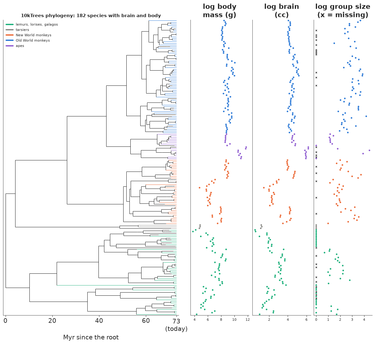
The phylogenetic structure of the traits is visible without any model: body and brain size come in clade-sized blocks (small-bodied lemurs, mouse lemurs and marmosets; large apes and baboons), and so, less sharply, does group size (large troops in the Old World monkeys; solitary animals - log group size 0 - in many lemurs, lorises and galagos). Any cross-species correlation between brain and group size can therefore come from a few deep splits. The crosses mark the 31 species with brain and body mass but no group size (section 9).
The 151 complete species are the regression data for sections 3-8. Every variable is logged and standardised on that sample; the covariance is scaled by the tree depth $T$, so that $R = C/T$ has ones on the diagonal (a correlation matrix, because the tree is ultrametric), and distances by the maximum $2T$.
cc = df.dropna(subset=["group_size"]).copy()
N = len(cc)


def standardise(x):
    return (x - x.mean()) / x.std()


B, M, G = (standardise(cc[c].to_numpy()) for c in ["log_brain", "log_body", "log_group_size"])
tips_cc = cc.tip.to_numpy()
R = C_full[np.ix_(tips_cc, tips_cc)] / T
Dn = D_full[np.ix_(tips_cc, tips_cc)] / (2 * T)
species = cc.index.to_numpy(dtype=object)
print(f"N = {N} species; corr(M, G) = {np.corrcoef(M, G)[0, 1]:.2f}; "
      f"mean off-diagonal correlation in R = {(R.sum() - N) / (N * (N - 1)):.2f}")

bounds = np.flatnonzero(cc.clade.to_numpy()[1:] != cc.clade.to_numpy()[:-1]) + 0.5
fig, axes = plt.subplots(1, 2, figsize=(11, 5))
for ax, mat, title in [(axes[0], R, "$R = C/T$: shared history (1 = same species)"),
                       (axes[1], Dn * 2 * T, "patristic distance $D$ (Myr)")]:
    im = ax.imshow(mat, cmap="viridis", interpolation="nearest")
    for b in bounds:
        ax.axhline(b, color="w", lw=0.5)
        ax.axvline(b, color="w", lw=0.5)
    ax.set(title=title, xticks=[], yticks=[], xlabel="species in tree order")
    fig.colorbar(im, ax=ax, shrink=0.8)
N = 151 species; corr(M, G) = 0.63; mean off-diagonal correlation in R = 0.30
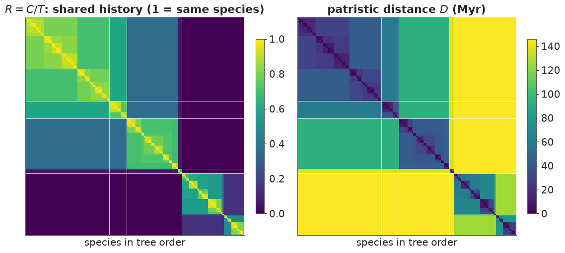
In tree order the covariance is a nest of blocks: the big block of the Old World monkeys,
the apes, the New World monkeys, the strepsirrhines (which share nothing with the rest:
the zero rows), and within them genera. This is the matrix we will put into pm.MvNormal.
3 · The i.i.d. regression, and a check that sees what it misses
$$B_i \sim \text{Normal}(a + \beta_M M_i + \beta_G G_i,\ \sigma)$$
Priors for standardised data: $a \sim \text{N}(0, 1)$, $\beta_M, \beta_G \sim \text{N}(0, 0.5)$ (a one-sd change in a predictor moving brain size by more than one sd is implausible, not impossible), $\sigma \sim \text{Exponential}(1)$. All models below share these; the only thing that changes is the covariance of the residuals.
def regression(kind, name=None):
    """Brain ~ body + group size with residual covariance of the given kind."""
    with pm.Model(coords={"species": species}, name=name or kind) as m:
        a = pm.Normal("a", 0, 1)
        bM = pm.Normal("bM", 0, 0.5)
        bG = pm.Normal("bG", 0, 0.5)
        mu = pm.Deterministic("mu", a + bM * M + bG * G, dims="species")
        if kind == "iid":
            sigma = pm.Exponential("sigma", 1)
            pm.Normal("B", mu, sigma, observed=B, dims="species")
            return m
        if kind == "bm":
            sigma = pm.Exponential("sigma", 1)
            K = sigma**2 * R
        elif kind == "lambda":
            sigma = pm.Exponential("sigma", 1)
            lam = pm.Beta("lam", 1, 1)
            K = sigma**2 * (lam * R + (1 - lam) * np.eye(N))
        elif kind == "ou":                      # GP with exponential kernel on patristic distance
            eta2 = pm.HalfNormal("eta2", 5)
            rho = pm.HalfNormal("rho", 5)
            K = eta2 * pm.math.exp(-rho * Dn) + 1e-6 * np.eye(N)
        elif kind == "ou_rate":                 # same model, sampled in (rate, rho)
            rate = pm.HalfNormal("rate", 1)
            rho = pm.HalfNormal("rho", 5)
            eta2 = pm.Deterministic("eta2", rate / rho)
            K = eta2 * pm.math.exp(-rho * Dn) + 1e-6 * np.eye(N)
        pm.MvNormal("B", mu, cov=K, observed=B, dims="species")
    return m


m_iid = regression("iid")
with m_iid:
    prior = pm.sample_prior_predictive(500, random_seed=RANDOM_SEED)
pp = prior.prior_predictive["iid::B"].to_numpy().ravel()
print(f"prior predictive of standardised log brain: 5-95% [{np.quantile(pp, 0.05):.1f}, {np.quantile(pp, 0.95):.1f}], "
      f"P(|B| > 5) = {np.mean(np.abs(pp) > 5):.3f}")
fits = {"iid": fit(m_iid)}
print(summ(fits["iid"], ["a", "bM", "bG", "sigma"]))
prior predictive of standardised log brain: 5-95% [-2.8, 2.8], P(|B| > 5) = 0.015
  iid: 1.4 s (incl. compile), divergences = 0
        mean     sd  eti89_lb  eti89_ub  ess_bulk  ess_tail  r_hat  mcse_mean  \
a      0.000  0.017    -0.027     0.028  4175.959  3177.462  1.001        0.0
bM     0.893  0.023     0.855     0.929  2263.894  2367.837  1.002        0.0
bG     0.123  0.023     0.087     0.160  2185.474  2781.644  1.002        0.0
sigma  0.217  0.013     0.198     0.238  3976.787  3149.547  1.002        0.0

       mcse_sd
a          0.0
bM         0.0
bG         0.0
sigma      0.0
The prior predictive is wide but not absurd (most mass within a few sds of the observed range). The i.i.d. fit says: at fixed body mass, a one-sd larger (log) group size goes with a 0.12 sd larger brain, with a tight interval that excludes zero. The social brain, confirmed?
A posterior predictive check tailored to the question: if the model is right, a species' residual should say nothing about its closest relative's residual. For every species $i$ let $\text{nn}(i)$ be the species at the smallest patristic distance, and compute $\text{corr}(r_i, r_{\text{nn}(i)})$ for the observed residuals $r = B - \mu$ and for residuals of data replicated from the posterior predictive, draw by draw.
D_cc = Dn.copy()
np.fill_diagonal(D_cc, np.inf)
nn = D_cc.argmin(axis=1)
print(f"median distance to the nearest relative: {np.median(D_cc.min(axis=1)) * 2 * T:.1f} Myr")


def sister_ppc(idata, model, n_thin=4):
    """corr(residual, nearest relative's residual): observed vs replicated, per posterior draw."""
    post = idata.posterior.isel(draw=slice(None, None, n_thin))
    with model:
        ppc = pm.sample_posterior_predictive(post, random_seed=RANDOM_SEED, progressbar=False)
    mu = post[f"{model.name}::mu"].stack(sample=("chain", "draw")).transpose("sample", ...).to_numpy()
    rep = ppc.posterior_predictive[f"{model.name}::B"].stack(sample=("chain", "draw")).transpose("sample", ...).to_numpy()

    def stat(r):
        r = r - r.mean(axis=1, keepdims=True)
        return (r * r[:, nn]).sum(1) / np.sqrt((r**2).sum(1) * (r[:, nn] ** 2).sum(1))

    return stat(B - mu), stat(rep - mu)


ppc_stats = {"iid": sister_ppc(fits["iid"], m_iid)}
obs, rep = ppc_stats["iid"]
print(f"observed: {np.median(obs):.2f}   replicated 90%: [{np.quantile(rep, 0.05):.2f}, "
      f"{np.quantile(rep, 0.95):.2f}]   P(rep >= obs) = {np.mean(rep >= obs):.3f}")
median distance to the nearest relative: 7.4 Myr
observed: 0.75   replicated 90%: [-0.17, 0.16]   P(rep >= obs) = 0.000
The residuals of close relatives are strongly correlated in the data and uncorrelated in every replicate: the i.i.d. model has not seen the tree, and the tree is in the residuals. Its tight interval for $\beta_G$ rests on 151 independent observations that do not exist.
4 · Brownian motion: the residual evolves along the tree
If the residual (brain size not explained by body size and group size) drifts as a Brownian motion along the branches, with rate $\sigma^2$ per unit of scaled time, then $$B \sim \text{MvNormal}(a + \beta_M M + \beta_G G,\ \sigma^2 R).$$ This is the Bayesian version of phylogenetic generalised least squares (PGLS; Grafen 1989), equivalent to Felsenstein's independent contrasts. Note what $a$ now is: the expected residual-adjusted brain size at the root, 73 million years ago.
Pagel's $\lambda$ (Pagel 1999) interpolates: multiply every off-diagonal element of $R$ by $\lambda \in [0, 1]$. $\lambda = 0$ is the i.i.d. model, $\lambda = 1$ Brownian motion; equivalently $\sigma^2(\lambda R + (1 - \lambda) I)$, a Brownian part plus a species-level "nugget" (on an ultrametric tree the two forms are the same, because $\text{diag}(R) = 1$). The nugget absorbs whatever is species-specific and not inherited: measurement error in a handful of skulls, recent rapid change, intraspecific variation.
for kind in ["bm", "lambda"]:
    fits[kind] = fit(regression(kind))
print(summ(fits["bm"], ["a", "bM", "bG", "sigma"]))
print(summ(fits["lambda"], ["a", "bM", "bG", "sigma", "lam"]))
bm: 2.6 s (incl. compile), divergences = 0
  lambda: 3.6 s (incl. compile), divergences = 0
        mean     sd  eti89_lb  eti89_ub  ess_bulk  ess_tail  r_hat  mcse_mean  \
a     -0.193  0.171    -0.469     0.078  5964.043  3409.835  1.000      0.002
bM     0.701  0.036     0.644     0.758  5202.148  3340.025  1.000      0.000
bG    -0.013  0.020    -0.046     0.019  5598.085  3235.417  1.002      0.000
sigma  0.401  0.024     0.366     0.439  5666.307  3152.754  1.001      0.000

       mcse_sd
a        0.002
bM       0.001
bG       0.000
sigma    0.000
        mean     sd  eti89_lb  eti89_ub  ess_bulk  ess_tail  r_hat  mcse_mean  \
a     -0.121  0.118    -0.312     0.065  3829.781  2848.231  1.001      0.002
bM     0.766  0.031     0.716     0.815  3165.246  3184.099  1.000      0.001
bG     0.026  0.019    -0.005     0.057  3506.857  3012.200  1.000      0.000
sigma  0.277  0.022     0.242     0.313  1904.451  1906.837  1.001      0.001
lam    0.954  0.018     0.922     0.977  1938.220  2151.454  1.002      0.000

       mcse_sd
a        0.002
bM       0.000
bG       0.000
sigma    0.000
lam      0.000
The group-size slope collapses: from 0.12 under i.i.d. to about zero under Brownian motion and to about 0.03 (interval touching zero) under $\lambda$. $\lambda$ itself is estimated at 0.95 (89% interval [0.92, 0.98]): residual brain size is almost entirely phylogenetic, with a small but clearly non-zero species-specific component. The book-keeping of uncertainty changes too, and not uniformly - see section 6.
5 · Ornstein-Uhlenbeck: a Gaussian process on the tree, and its ridge
Brownian motion lets a trait wander without bound. The Ornstein-Uhlenbeck process
pulls it back towards an optimum with strength $\alpha$. On an ultrametric tree, with the
root at stationarity, the covariance is
$$K_{ij} = \eta^2 \exp(-\rho\, D_{ij} / 2T),$$
which is exactly the exponential (Matérn-1/2) Gaussian-process kernel of E05 with
patristic distance in place of Euclidean distance; $\rho = 2T\alpha$ and the
phylogenetic half-life is $\ln 2 / \alpha = 2T \ln 2 / \rho$. (It is the model rethinking
fits with cov_GPL1.) First attempt: weakly informative half-normal priors on $\eta^2$ and
$\rho$ separately. Both OU fits use target_accept=0.95: at the default 0.8 they produce a
few divergences, a first sign of awkward geometry.
m_ou = regression("ou")
fits["ou"] = fit(m_ou, target_accept=0.95)
print(summ(fits["ou"], ["bM", "bG", "eta2", "rho"]))
e2, rh = draws(fits["ou"], "ou::eta2"), draws(fits["ou"], "ou::rho")
print(f"corr(log eta2, log rho) = {np.corrcoef(np.log(e2), np.log(rh))[0, 1]:.3f};  "
      f"eta2*rho: median {np.median(e2 * rh):.3f}, 90% [{np.quantile(e2 * rh, 0.05):.3f}, {np.quantile(e2 * rh, 0.95):.3f}]")
  ou: 13.5 s (incl. compile), divergences = 0
       mean     sd  eti89_lb  eti89_ub  ess_bulk  ess_tail  r_hat  mcse_mean  \
bM    0.719  0.041     0.656     0.784   993.009  1150.842  1.003      0.001
bG   -0.010  0.020    -0.041     0.023  2476.878  2238.867  1.001      0.000
eta2  0.760  1.261     0.085     3.080   288.115   555.147  1.007      0.059
rho   0.809  0.761     0.053     2.270   282.235   557.010  1.007      0.045

      mcse_sd
bM      0.001
bG      0.000
eta2    0.108
rho     0.029
corr(log eta2, log rho) = -0.994;  eta2*rho: median 0.171, 90% [0.138, 0.216]
The divergences are gone at target_accept=0.95, but look at the effective sample sizes of $\eta^2$ and $\rho$
(about 300 out of 4000, against over a thousand for the slopes) and at their correlation on
the log scale: $-0.99$. The posterior is a thin ridge (a straight line on the log scale) along which
$\eta^2 \rho$ is constant. The reason is a first-order expansion: for small $\rho$,
$$\eta^2 e^{-\rho D_{ij}/2T} \approx \eta^2 - \eta^2\rho \,\tfrac{D_{ij}}{2T}
= \underbrace{\eta^2(1-\rho)}_{\text{shared by all species}} + \eta^2\rho\, R_{ij},$$
using $D_{ij}/2T = 1 - R_{ij}$. The first term is a random intercept that the intercept $a$
soaks up; what remains is Brownian motion with rate $\eta^2\rho$. The data pin down the
product, the Brownian rate, and say little about $\rho$ unless the pull towards the
optimum is strong enough to show in 73 Myr. (This is the phylogenetic cousin of Zhang's
2004 result that only $\eta^2/\ell$ is consistently estimable for a Matérn GP.)
Fix: sample along and across the ridge. Put the prior on the identified quantity, $\text{rate} = \eta^2\rho \sim \text{HalfNormal}(1)$, and on $\rho$; $\eta^2 = \text{rate}/\rho$ becomes a deterministic. Same family of models, much better geometry.
m_ou_rate = regression("ou_rate")
fits["ou_rate"] = fit(m_ou_rate, target_accept=0.95)
print(summ(fits["ou_rate"], ["bM", "bG", "rate", "rho", "eta2"]))
  ou_rate: 7.7 s (incl. compile), divergences = 0
       mean     sd  eti89_lb  eti89_ub  ess_bulk  ess_tail  r_hat  mcse_mean  \
bM    0.739  0.043     0.669     0.810  1616.433  1990.397  1.005      0.001
bG   -0.006  0.021    -0.038     0.027  2803.680  2295.124  1.003      0.000
rate  0.185  0.027     0.147     0.231  1586.154  1893.884  1.003      0.001
rho   1.596  0.956     0.292     3.266   942.831  1072.296  1.007      0.030
eta2  0.222  0.718     0.063     0.550  1021.623  1070.343  1.006      0.016

      mcse_sd
bM      0.001
bG      0.000
rate    0.001
rho     0.019
eta2 0.266 rate_r, rho_r, e2_r = (draws(fits["ou_rate"], "ou_rate::" + v) for v in ["rate", "rho", "eta2"])
with m_ou_rate:
prior_rho = pm.draw(m_ou_rate["ou_rate::rho"], 20000, random_seed=RANDOM_SEED)
fig, axes = plt.subplots(1, 3, figsize=(15, 4.2))
axes[0].scatter(np.log(rh), np.log(e2), s=2, alpha=0.3, color=GREY, label="($\\eta^2$, $\\rho$) priors")
axes[0].scatter(np.log(rho_r), np.log(e2_r), s=2, alpha=0.3, color=BLUE, label="(rate, $\\rho$) priors")
xs = np.linspace(-4, 2, 50)
axes[0].plot(xs, np.log(np.median(rate_r)) - xs, color="k", lw=1, ls="--", label="$\\eta^2\\rho$ = const")
axes[0].set(xlabel="log $\\rho$", ylabel="log $\\eta^2$")
axes[0].set_title("posterior: a ridge", fontsize=11)
axes[0].legend(fontsize=8, markerscale=4)
axes[1].hist(e2 * rh, bins=50, density=True, alpha=0.6, color=GREY, label="($\\eta^2$, $\\rho$) priors")
axes[1].hist(rate_r, bins=50, density=True, alpha=0.6, color=BLUE, label="(rate, $\\rho$) priors")
axes[1].set(xlabel="Brownian rate $\\eta^2\\rho$")
axes[1].set_title("identified: nearly the same under both", fontsize=11)
axes[1].legend(fontsize=8)
half_life = lambda r: 2 * T * np.log(2) / r
bins = np.logspace(0, 4, 60)
axes[2].hist(half_life(prior_rho), bins=bins, density=True, histtype="step", color="k", label="prior on $\\rho$ (same in both)")
axes[2].hist(half_life(rh), bins=bins, density=True, histtype="step", lw=2, color=GREY, label="posterior, ($\\eta^2$, $\\rho$)")
axes[2].hist(half_life(rho_r), bins=bins, density=True, alpha=0.5, color=BLUE, label="posterior, (rate, $\\rho$)")
axes[2].axvline(T, color=ORANGE, lw=1.5, label=f"tree depth {T:.0f} Myr")
axes[2].set(xscale="log", xlabel="phylogenetic half-life (Myr)")
axes[2].set_title("weakly identified: depends on the prior", fontsize=11)
axes[2].legend(fontsize=8);
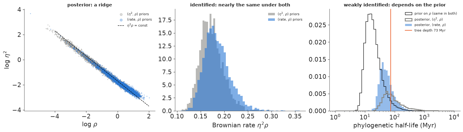
Left: the two posteriors live on the same ridge (dashed line: constant rate); the reparameterised sampler only moves more easily along it, which is why its effective sample sizes for $\rho$ and $\eta^2$ are over three times as large (and the reparameterised fit is faster). Middle: the Brownian rate is nearly the same under both parameterisations - that is what the data know. Right: the half-life is where the prior shows. The data rule out very short half-lives (a strong pull to an optimum, which would make distant relatives uncorrelated sooner than they are) but cannot tell a half-life comparable to the tree depth from an infinite one, which is Brownian motion. The prior on $\rho$ is the same HalfNormal(5) in both models, yet the posteriors of the half-life differ: along a ridge, the prior on the other coordinate (HalfNormal(5) on $\eta^2$ vs HalfNormal(1) on $\eta^2\rho$) decides where the mass sits, and the vague $\eta^2$ prior lets the chain wander out to half-lives of thousands of Myr, which is Brownian motion by another name. The honest report is "consistent with Brownian motion; if there is an optimum, the pull is slow", not a number for $\alpha$.
6 · What happened to the slopes
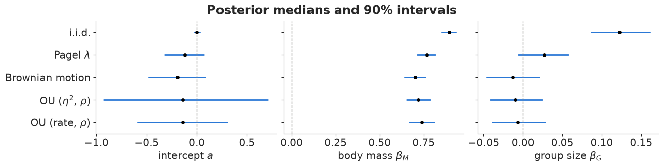
Five models, three coefficients. The two OU fits are the same likelihood with different priors; they agree on the slopes but not on the intercept, because a small $\rho$ (far out along the ridge) is a large random intercept - see the expansion above - and the vague $\eta^2$ prior lets the chain go there.
order_models = ["iid", "lambda", "bm", "ou", "ou_rate"]
labels = {"iid": "i.i.d.", "lambda": "Pagel $\\lambda$", "bm": "Brownian motion",
          "ou": "OU ($\\eta^2$, $\\rho$)", "ou_rate": "OU (rate, $\\rho$)"}
fig, axes = plt.subplots(1, 3, figsize=(13, 3.2), sharey=True)
rows = []
for ax, var, xl in zip(axes, ["a", "bM", "bG"], ["intercept $a$", "body mass $\\beta_M$", "group size $\\beta_G$"]):
    for k, mname in enumerate(order_models):
        x = draws(fits[mname], f"{mname}::{var}")
        lo, med, hi = np.quantile(x, [0.05, 0.5, 0.95])
        ax.plot([lo, hi], [k, k], color=BLUE, lw=2)
        ax.scatter(med, k, color="k", zorder=3, s=15)
        rows.append({"model": mname, "coef": var, "median": med, "sd": x.std()})
    ax.axvline(0, color=GREY, ls="--", lw=1)
    ax.set(xlabel=xl)
axes[0].set(yticks=range(len(order_models)), yticklabels=[labels[m] for m in order_models], ylim=(len(order_models) - 0.5, -0.5))
fig.suptitle("Posterior medians and 90% intervals")
sd_tab = pd.DataFrame(rows).pivot(index="model", columns="coef", values="sd").loc[order_models]
print("posterior sd, relative to the i.i.d. model:")
print((sd_tab / sd_tab.loc["iid"]).round(2));
posterior sd, relative to the i.i.d. model:
coef         a    bG    bM
model
iid       1.00  1.00  1.00
lambda    6.86  0.85  1.33
bm        9.93  0.89  1.56
ou       28.44  0.89  1.76
ou_rate  16.75  0.91  1.88
Three lessons in one figure.
- The group-size effect is a phylogenetic artefact, mostly. Once shared ancestry is modelled, $\beta_G$ is within a few hundredths of zero in every tree model. The i.i.d. estimate of 0.12 came from a few deep contrasts (large-bodied, big-group Old World monkeys vs small-group strepsirrhines) counted once per species.
- Uncertainty does not simply grow. The intercept's sd grows 7-10x under $\lambda$ and Brownian motion (and 16-29x under OU, whose ridge adds a near-free random intercept): the mean brain size of primates is, in effect, estimated from a handful of deep lineages, and $a$ is now a statement about the root. $\beta_M$'s sd grows by 30-90%. $\beta_G$'s shrinks by 10-15%: in a tree model its information comes from differences between close relatives (a contrast between two sister species is nearly independent of everything else), there are many of those, and the residual noise within them is smaller than the i.i.d. $\sigma$. Which coefficients widen depends on where on the tree their predictor varies.
- The body-mass slope drops from about 0.89 to 0.70-0.77: the famous "brain scales with body mass to the 3/4 power" is partly between-clade grade shifts, and within clades the scaling is shallower (a known result in comparative neurobiology).
7 · Which covariance? Leave-one-out for a correlated likelihood
To compare the models by expected predictive accuracy we want PSIS-LOO. With an i.i.d.
likelihood the log-likelihood splits into one term per species and az.loo does the rest.
With pm.MvNormal it does not split. Two tempting shortcuts and the right answer:
Wrong 1: use what PyMC gives you. pm.compute_log_likelihood returns the log density
of the whole vector per draw - one "observation". LOO over it leaves out all the data.
m_bm = regression("bm")
ll_joint = fits["bm"].copy()
with m_bm:
    pm.compute_log_likelihood(ll_joint, progressbar=False)
print(dict(ll_joint.log_likelihood["bm::B"].sizes))
print(az.loo(ll_joint))
{'chain': 4, 'draw': 1000}
Computed from 4000 posterior samples and 1.0 observations log-likelihood matrix.

         Estimate       SE
elpd_loo    73.24     0.00
p_loo        3.01        -

There has been a warning during the calculation. Please check the results.
------

Pareto k diagnostic values:
                         Count   Pct.
(-Inf, 0.70]   (good)        0    0.0%
   (0.70, 1]   (bad)         0    0.0%
    (1, Inf)   (very bad)    1  100.0%
One observation, Pareto $k > 1$: meaningless, and the dimension of the log-likelihood array tells you so.
Wrong 2: use the marginal density of each species, $\text{N}(B_i \mid \mu_i, K_{ii})$.
That has one term per species, and az.loo will happily process it. But it scores the
prediction of species $i$ without using its relatives, which is not what the model would
do if $i$ were left out and is not the same model at all.
Right: the conditional (leave-one-out) predictive. For $y \sim \text{MvNormal}(\mu, K)$, the distribution of $y_i$ given all the others is normal, and with the precision matrix $Q = K^{-1}$ it has a closed form (Sundararajan & Keerthi 2001; Bürkner, Gabry & Vehtari 2021): $$y_i \mid y_{-i} \sim \text{N}\!\left(y_i - \frac{g_i}{Q_{ii}},\ \frac{1}{Q_{ii}}\right), \qquad g = Q(y - \mu).$$ So one inverse per posterior draw gives all $N$ pointwise log densities $\log p(y_i \mid y_{-i}, \theta) = -\tfrac12\log 2\pi + \tfrac12 \log Q_{ii} - \tfrac12 g_i^2/Q_{ii}$, and PSIS then reweights the draws from "fitted with $i$" to "fitted without $i$" as usual. (That second step is still needed: the formula conditions on $y_{-i}$ at fixed parameters, PSIS handles the parameters.)
def covariance_draws(mname):
    p = lambda v: draws(fits[mname], f"{mname}::{v}")
    if mname == "iid":
        s = p("sigma")
        return lambda k: s[k] ** 2 * np.eye(N)
    if mname == "bm":
        s = p("sigma")
        return lambda k: s[k] ** 2 * R
    if mname == "lambda":
        s, lam = p("sigma"), p("lam")
        return lambda k: s[k] ** 2 * (lam[k] * R + (1 - lam[k]) * np.eye(N))
    e2, rho = p("eta2"), p("rho")
    return lambda k: e2[k] * np.exp(-rho[k] * Dn) + 1e-6 * np.eye(N)


def pointwise_loglik(mname):
    """(conditional LOO log density, marginal log density), each draws x species."""
    mu = draws(fits[mname], f"{mname}::mu")
    K_of = covariance_draws(mname)
    S = len(mu)
    ll_cond, ll_marg = np.empty((S, N)), np.empty((S, N))
    for k in range(S):
        K = K_of(k)
        Q = np.linalg.inv(K)
        q, g = np.diag(Q), Q @ (B - mu[k])
        ll_cond[k] = -0.5 * np.log(2 * np.pi) + 0.5 * np.log(q) - 0.5 * g**2 / q
        kd = np.diag(K)
        ll_marg[k] = -0.5 * np.log(2 * np.pi * kd) - 0.5 * (B - mu[k]) ** 2 / kd
    return ll_cond, ll_marg


def loo_from(mname, ll):
    n_chain = fits[mname].posterior.sizes["chain"]
    tree = xr.DataTree.from_dict({
        "posterior": fits[mname].posterior.to_dataset(),
        "log_likelihood": xr.Dataset({"B": (("chain", "draw", "species"), ll.reshape(n_chain, -1, N))}),
    })
    res = az.loo(tree, pointwise=True)
    res.log_weights = None       # keep only what az.compare needs
    return res


loo_cond, loo_marg = {}, {}
t0 = time.time()
for mname in ["iid", "lambda", "bm", "ou_rate"]:
    llc, llm = pointwise_loglik(mname)
    loo_cond[mname], loo_marg[mname] = loo_from(mname, llc), loo_from(mname, llm)
print(f"4 models x 4000 draws x one {N}x{N} inverse: {time.time() - t0:.1f} s")
cmp_cond = az.compare(loo_cond)
cmp_marg = az.compare(loo_marg)
print("RIGHT - conditional (leave-one-out) predictive:")
print(cmp_cond[["rank", "elpd", "p", "elpd_diff", "dse", "weight"]].round(1))
print("\nWRONG - marginal pointwise densities:")
print(cmp_marg[["rank", "elpd", "p", "elpd_diff", "dse", "weight"]].round(1))
print("\nPareto k > 0.7 (conditional):", {m: int((loo_cond[m].pareto_k > 0.7).sum()) for m in loo_cond})
4 models x 4000 draws x one 151x151 inverse: 3.6 s
RIGHT - conditional (leave-one-out) predictive:
         rank   elpd     p  elpd_diff   dse  weight
lambda      0  130.0   4.4        0.0   0.0     1.0
bm          1   90.0  12.5      -40.0  21.0     0.0
ou_rate     2   90.0  13.0      -40.0  19.0     0.0
iid         3   20.0   4.1     -110.0  11.0     0.0

WRONG - marginal pointwise densities:
         rank   elpd     p  elpd_diff  dse  weight
iid         0   20.0   4.1        0.0  0.0     1.0
lambda      1  -90.0  45.3     -100.0  8.6     0.0
bm          2 -120.0  36.7     -130.0  9.1     0.0
ou_rate     3 -150.0  79.1     -170.0  8.7     0.0

Pareto k > 0.7 (conditional): {'iid': 0, 'lambda': 0, 'bm': 1, 'ou_rate': 2}
The two tables rank the models in opposite order. The marginal version prefers the i.i.d. model by a huge margin - of course: scoring each species without its relatives, the tree models' residual variance $K_{ii}$ is larger (it must also cover the deep between-clade variation that the relatives would have explained), so each marginal density is flatter. The conditional version uses the relatives, as a phylogenetic model predicting a left-out species would, and ranks $\lambda$ first, Brownian motion and OU (which give near-identical fits, as the ridge analysis predicted) about 40 elpd behind, and the i.i.d. model last by more than 100. (The $\lambda$-vs-BM difference of about 40 has a standard error of about 20: clear, not overwhelming.) The i.i.d. model's conditional and marginal elpd are identical, as they must be.
Why does $\lambda$ beat pure Brownian motion so clearly? Look at where the difference comes from, species by species.
elpd_i = {m: np.asarray(loo_cond[m].elpd_i) for m in loo_cond}
diff = elpd_i["lambda"] - elpd_i["bm"]
nn_dist = D_cc.min(axis=1) * 2 * T
fig, ax = plt.subplots(figsize=(8, 4))
ax.scatter(nn_dist, diff, s=14, c=[clades[c][1] for c in cc.clade])
ax.axhline(0, color=GREY, lw=1)
ax.set(xscale="log", xlabel="distance to the nearest relative in the data (Myr, log scale)",
       ylabel="elpd$_i$($\\lambda$) - elpd$_i$(BM)",
       title="Where Pagel's $\\lambda$ beats Brownian motion")
for k, i in enumerate(np.argsort(diff)[::-1][:3]):
    ax.annotate(species[i].replace("_", " "), (nn_dist[i], diff[i]), fontsize=7,
                xytext=(6, -9 * k if k < 2 else 4), textcoords="offset points")
print(cc.loc[species[np.argsort(diff)[-2:]], ["brain", "body", "group_size"]])
close = nn_dist < 2
print(f"species with a relative < 2 Myr away: {close.sum()}, they account for "
      f"{diff[close].sum():.1f} of the total elpd difference {diff.sum():.1f}");
                            brain    body  group_size
name
Cercocebus_torquatus       105.99  7485.0       26.85
Cercocebus_torquatus_atys   94.68  8600.0       35.00
species with a relative < 2 Myr away: 14, they account for 34.9 of the total elpd difference 38.6
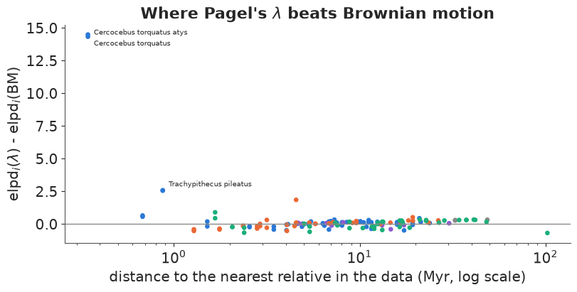
The gain is concentrated in species with a very close relative in the data: the 14 species with a relative less than 2 Myr away carry 35 of the 39 elpd units, and one pair carries most of it - Cercocebus torquatus and its subspecies C. t. atys, 0.35 Myr apart in the tree, where the subspecies is the heavier of the two but has the smaller brain. Pure Brownian motion predicts each of them almost exactly from the other, with a tiny predictive variance, and that overconfident prediction is punished hard. The nugget $1 - \lambda \approx 0.05$ puts a floor under the predictive variance (a different sample of skulls, a real recent change). This is also why Brownian motion and OU have a large $p_{\text{loo}}$ and one or two Pareto $k$ values above 0.7: a few species are each essentially predicted by one sister. An OU model with a nugget is the natural next model (Try it yourself, 2).
The posterior predictive check from section 3, now for all four covariances:
for mname in ["lambda", "bm", "ou_rate"]:
    ppc_stats[mname] = sister_ppc(fits[mname], regression(mname))
fig, axes = plt.subplots(1, 4, figsize=(14, 3.4), sharex=True, sharey=True)
for ax, mname in zip(axes, ["iid", "lambda", "bm", "ou_rate"]):
    obs, rep = ppc_stats[mname]
    ax.scatter(rep, obs, s=3, alpha=0.4, color=BLUE)
    ax.plot([-0.5, 1], [-0.5, 1], color="k", lw=1)
    ax.set(title=f"{labels[mname]}\nP(rep $\\geq$ obs) = {np.mean(rep >= obs):.2f}", xlabel="replicated")
axes[0].set_ylabel("observed");
fig.suptitle("corr(residual, nearest relative's residual): one point per posterior draw");
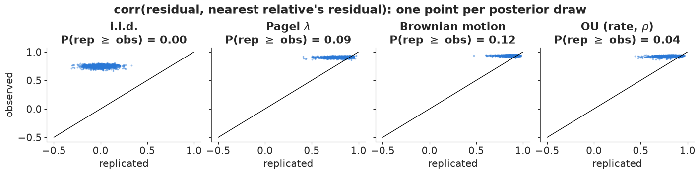
Each point is one posterior draw: the observed statistic against the one from data replicated under that draw. For the i.i.d. model all points sit far above the diagonal (observed 0.75, replicated around 0). For the three tree models the observed residual correlation is about 0.9 and the replicated values reach it: most of the phylogenetic signal is reproduced, although the observed value sits in the upper tail of the replicates (posterior predictive p-values 0.04-0.12, lowest for OU). Close relatives are even a little more alike than these models expect - a hint that rates of evolution are not constant across the tree (Try it yourself, 1).
8 · Cost: dense covariances, whitening, and the tree's sparse precision
Every gradient of an MvNormal with a parameter-dependent covariance costs a Cholesky
factorisation, $O(N^3)$: trivial at $N = 151$, painful at a few thousand species (a
mammal or bird tree). Two remedies.
Whitening, when the correlation matrix is fixed (Brownian motion): factor $R = LL^\top$ once, and $L^{-1}B \sim \text{N}(L^{-1}\mu, \sigma^2 I)$ is an ordinary independent-normal likelihood with the same posterior.
L = np.linalg.cholesky(R)
Bw = solve_triangular(L, B, lower=True)
Xw = solve_triangular(L, np.column_stack([np.ones(N), M, G]), lower=True)
with pm.Model(name="bm_white") as m_white:
    a = pm.Normal("a", 0, 1)
    bM = pm.Normal("bM", 0, 0.5)
    bG = pm.Normal("bG", 0, 0.5)
    sigma = pm.Exponential("sigma", 1)
    pm.Normal("Bw", Xw[:, 0] * a + Xw[:, 1] * bM + Xw[:, 2] * bG, sigma, observed=Bw)
fit_white = fit(m_white)
for v in ["a", "bM", "bG", "sigma"]:
    print(f"{v:6s} dense: {draws(fits['bm'], 'bm::' + v).mean():+.3f} ± {draws(fits['bm'], 'bm::' + v).std():.3f}"
          f"   whitened: {draws(fit_white, 'bm_white::' + v).mean():+.3f} ± {draws(fit_white, 'bm_white::' + v).std():.3f}")
  bm_white: 0.5 s (incl. compile), divergences = 0
a      dense: -0.193 ± 0.171   whitened: -0.193 ± 0.171
bM     dense: +0.701 ± 0.036   whitened: +0.701 ± 0.036
bG     dense: -0.013 ± 0.020   whitened: -0.013 ± 0.020
sigma  dense: +0.401 ± 0.024   whitened: +0.401 ± 0.024
Identical posteriors (to Monte Carlo error), and the per-gradient cost is now that of an
i.i.d. regression. At this size compile time dominates the wall-clock numbers printed by
fit; the saving is in the $O(N^3)$ factorisation, which the whitened model never does.
The tree's precision is sparse. The dense $C$ hides a simple structure. Add the internal nodes as variables: each node is its parent plus an independent increment, $x_c \sim \text{N}(x_{p(c)}, \sigma^2 \ell_c)$. The joint density of all nodes then has a precision matrix with a non-zero only for each (parent, child) pair: the weighted graph Laplacian of the tree with weights $1/\ell_c$, with the root held fixed. That is an intrinsic Gaussian Markov random field on a graph - the ICAR of E18, on a tree instead of a map. Inverting it and keeping the tip block gives back $C$:
Qt = np.zeros((n_node, n_node))
for p, c in edge:
    w = 1.0 / blen[c]
    Qt[p, p] += w
    Qt[c, c] += w
    Qt[p, c] -= w
    Qt[c, p] -= w
keep = np.setdiff1d(np.arange(n_node), [root])            # condition on the root (= 0)
cov_nodes = np.linalg.inv(Qt[np.ix_(keep, keep)])
tip_block = cov_nodes[:n_tip, :n_tip]                      # tips are nodes 0..300, before the root
print(f"max |inv(Q_tree)[tips] - C| = {np.abs(tip_block - C_full).max():.1e}")
print(f"non-zeros: precision {np.count_nonzero(Qt[np.ix_(keep, keep)]) / keep.size**2:.2%} of {keep.size}^2, "
      f"covariance C {np.count_nonzero(C_full) / n_tip**2:.0%} of {n_tip}^2")
max |inv(Q_tree)[tips] - C| = 5.0e-11
non-zeros: precision 0.50% of 594^2, covariance C 56% of 301^2
Half a percent of the precision is non-zero, against 56% of the covariance (the zeros in
$C$ are only the pairs across the root). Two practical consequences: likelihoods on trees
can be evaluated in $O(N)$ by a recursion (Felsenstein's pruning algorithm; the
phylolm trick of Ho & Ané 2014), and in a PPL we can simply sample the internal nodes,
non-centred, which costs one parameter per node but no matrix algebra at all. The next
section uses the second option for a trait we have not fully observed.
9 · Missing group sizes: impute them on the tree
Sections 3-8 used the 151 species with all three traits and silently dropped 31 species with a brain and a body mass but no group size. Dropping is not free: it throws away their brain and body information, and it is only harmless if the missingness is unrelated to the outcome. The Bayesian alternative treats the missing group sizes as parameters with a model of their own - and the natural model for a trait of a species is, again, evolution on the tree.
First, is the missingness innocent?
miss = df.group_size.isna()
print(pd.DataFrame({
    "n": [(~miss).sum(), miss.sum()],
    "median research effort": [df.research_effort[~miss].median(), df.research_effort[miss].median()],
    "median body mass (g)": [df.body[~miss].median(), df.body[miss].median()],
}, index=["group size observed", "group size missing"]))
print(df[miss].clade.value_counts().to_string())
                       n  median research effort  median body mass (g)
group size observed  151                    18.0                4450.0
group size missing    31                     7.5                3532.0
clade
Old World monkeys           12
lemurs, lorises, galagos    10
New World monkeys            5
apes                         4
The species without a group size are spread over all the clades, but they are the little-studied ones: median research effort (number of publications) 7.5 against 18. So the data are probably not missing completely at random. An imputation model that uses the tree assumes they are missing at random given the phylogeny (and, through the joint model, given brain size): a missing species' group size is predicted from its relatives'. That is a much weaker assumption than complete-case analysis makes, but it is still an assumption.
The model, on all 182 species:
- group size evolves as Brownian motion on the tree: internal nodes are sampled
non-centred, $x_c = x_{p(c)} + \sigma_G \sqrt{\ell_c}\, z_c$; the observed tip value is
$G_i \sim \text{N}(x_{p(i)},\ \sqrt{\sigma_G^2 \ell_i + \tau_G^2})$, a terminal branch
plus a nugget $\tau_G$. Passing a vector with
NaNs asobservedmakes PyMC create the 31 missing tips as parameters (automatic imputation). - brain size: the $\lambda$ regression of section 4, with the completed $G$.
tips_all = df.tip.to_numpy()
N2 = len(df)
B2, M2 = (standardise(df[c].to_numpy()) for c in ["log_brain", "log_body"])
g_raw = df.log_group_size.to_numpy()
G2 = (g_raw - np.nanmean(g_raw)) / np.nanstd(g_raw)
R2 = C_full[np.ix_(tips_all, tips_all)] / T

# internal nodes above the 182 tips, root first; the branch above each non-root node
inner = sorted({int(a) for t in tips_all for a in np.flatnonzero(Anc[t]) if a >= n_tip} | {root},
               key=lambda n: depth[n])
pos = {n: k for k, n in enumerate(inner)}
branch = inner[1:]
A_inner = Anc[np.ix_(inner, branch)]                       # node x branch ancestry, root row = 0
bl_inner = blen[branch] / T
tip_parent = np.array([pos[parent[t]] for t in tips_all])
bl_tip = blen[tips_all] / T
print(f"{len(inner)} internal nodes above the {N2} species; {np.isnan(G2).sum()} group sizes missing")

with pm.Model(coords={"species": df.index.to_numpy(dtype=object)}, name="impute") as m_imp:
    g0 = pm.Normal("g_root", 0, 1)
    sigma_G = pm.Exponential("sigma_G", 1)
    tau_G = pm.Exponential("tau_G", 2)
    z = pm.Normal("z", 0, 1, shape=len(branch))
    x_inner = g0 + pm.math.dot(A_inner, sigma_G * np.sqrt(bl_inner) * z)
    G_full = pm.Normal("G", x_inner[tip_parent], pm.math.sqrt(sigma_G**2 * bl_tip + tau_G**2), observed=G2)
    a = pm.Normal("a", 0, 1)
    bM = pm.Normal("bM", 0, 0.5)
    bG = pm.Normal("bG", 0, 0.5)
    sigma = pm.Exponential("sigma", 1)
    lam = pm.Beta("lam", 1, 1)
    pm.MvNormal("B", a + bM * M2 + bG * G_full, cov=sigma**2 * (lam * R2 + (1 - lam) * np.eye(N2)), observed=B2)
fit_imp = fit(m_imp, target_accept=0.9)
print(summ(fit_imp, ["g_root", "sigma_G", "tau_G", "a", "bM", "bG", "sigma", "lam"]))
s_miss = summ(fit_imp, ["G_unobserved"])
print(f"imputed values: max r_hat {s_miss['r_hat'].max():.3f}, min bulk ESS {s_miss['ess_bulk'].min():.0f}")
264 internal nodes above the 182 species; 31 group sizes missing
  impute: 40.7 s (incl. compile), divergences = 0
          mean     sd  eti89_lb  eti89_ub  ess_bulk  ess_tail  r_hat  \
g_root  -0.732  0.416    -1.397    -0.092   336.962   532.603  1.008
sigma_G  1.127  0.114     0.947     1.313   865.682  1105.082  1.002
tau_G    0.279  0.042     0.214     0.350   846.267  1299.911  1.002
a       -0.146  0.116    -0.326     0.038  6247.663  3018.238  1.000
bM       0.735  0.030     0.685     0.783  5107.709  3158.962  1.002
bG       0.033  0.020     0.002     0.065  4807.765  3584.995  1.000
sigma    0.277  0.022     0.244     0.315  3942.446  2793.207  1.001
lam      0.948  0.017     0.917     0.972  3787.562  2791.597  1.000

         mcse_mean  mcse_sd
g_root       0.023    0.012
sigma_G      0.004    0.002
tau_G        0.001    0.001
a            0.001    0.002
bM           0.000    0.000
bG           0.000    0.000
sigma        0.000    0.000
lam          0.000    0.000
imputed values: max r_hat 1.003, min bulk ESS 1959
Gm = draws(fit_imp, "impute::G_unobserved")
mu_g, sd_g = np.nanmean(g_raw), np.nanstd(g_raw)
imp_groups = np.exp(Gm * sd_g + mu_g)
mi = np.flatnonzero(np.isnan(G2))
o = np.argsort(np.median(imp_groups, axis=0))
fig, axes = plt.subplots(1, 2, figsize=(13, 7), gridspec_kw={"width_ratios": [2, 1]})
ax = axes[0]
for row, j in enumerate(o):
sp = df.index[mi[j]]
lo, med, hi = np.quantile(imp_groups[:, j], [0.05, 0.5, 0.95])
ax.plot([lo, hi], [row, row], color=clades[df.clade.iloc[mi[j]]][1], lw=2)
ax.scatter(med, row, color="k", s=10, zorder=3)
mates = df[(df.genus == df.genus.iloc[mi[j]]) & ~miss].group_size
ax.scatter(mates, np.full(len(mates), row), marker="|", color=GREY, s=40)
ax.set(xscale="log", yticks=range(len(o)), xlabel="group size (log scale)",
title="Imputed group size (90%); grey ticks: observed species of the same genus")
ax.title.set_fontsize(10)
ax.set_yticklabels([df.index[mi[j]].replace("_", " ") for j in o], fontsize=7)
ax = axes[1]
for k, (lab, x) in enumerate([("complete cases (151), $\\lambda$", draws(fits["lambda"], "lambda::bG")),
("imputed on the tree (182)", draws(fit_imp, "impute::bG")),
("complete cases, i.i.d.", draws(fits["iid"], "iid::bG"))]):
ax.hist(x, bins=60, density=True, alpha=0.55, label=lab, color=[BLUE, ORANGE, GREY][k])
ax.axvline(0, color="k", lw=1)
ax.set(xlabel="group-size slope $\\beta_G$")
ax.set_title("The social-brain slope", fontsize=10)
ax.legend(fontsize=8);
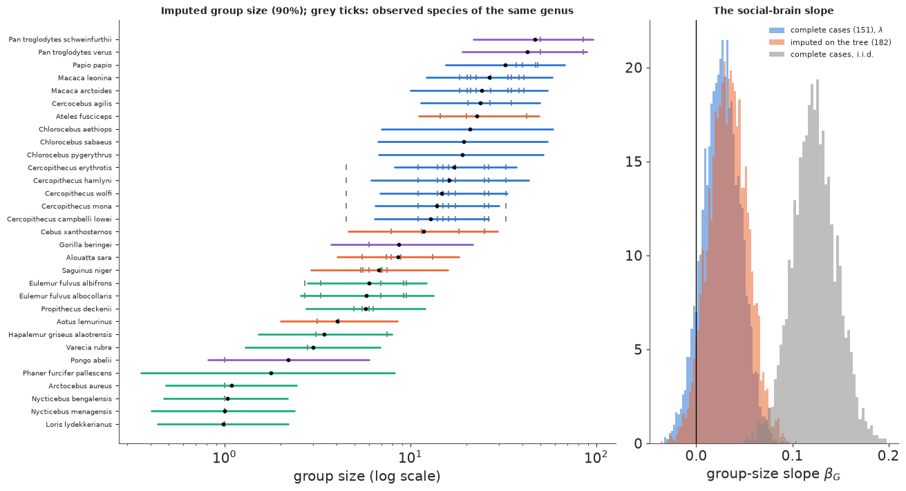
The imputations look like what a primatologist would guess from the relatives: the slow lorises, the slender loris and the golden potto sit at about 1 (their observed relatives are solitary), the two chimpanzee subspecies at about 45 next to the observed chimpanzees, the Cercopithecus guenons among their many observed congeners. The three Chlorocebus (vervet) species have no observed genus-mate and borrow from the other guenons. Most intervals span a factor of 4-8 from end to end - the nugget $\tau_G$ and the terminal branch set that floor - and the fork-marked lemur Phaner furcifer pallescens, with no observed genus-mate and a long terminal branch, over 20. And the substantive answer is unchanged: with the 31 extra species the group-size slope moves from 0.027 to 0.034 and its 89% interval still starts at zero, a far cry from the i.i.d. 0.12.
Two caveats. The imputation model for group size does not use body mass (large-bodied species tend to live in larger groups): adding $M$ as a predictor of $G$ would sharpen the imputations. And the brain model feeds back into the imputations (through $\beta_G$) - here weakly, because $\beta_G$ is near zero.
10 · Summary and connections
| Question | Answer here |
|---|---|
| Are species independent data points? | No: close relatives' residuals correlate (section 3's check, $\lambda \approx 0.95$) |
| Where does the covariance come from? | Shared branch length, $C = A\,\text{diag}(\ell)A^\top$; distance $D = 2(T - C)$ on an ultrametric tree |
| Does the social-brain slope survive? | Not in this form: 0.12 (i.i.d.) becomes -0.01 to 0.03, with intervals that include or touch zero |
| Does modelling correlation always widen intervals? | No: the intercept's sd grows ~10x, $\beta_G$'s shrinks slightly - it depends where the predictor varies on the tree |
| Brownian motion or OU? | Indistinguishable: the OU half-life is not identified beyond "not short"; report the Brownian rate $\eta^2\rho$ |
| How to compare correlated-likelihood models? | Conditional LOO from $Q = K^{-1}$ plus PSIS; the marginal shortcut reverses the ranking |
| What about missing traits? | Impute them on the tree inside the model (latent internal nodes = a sparse GMRF) |
Connections. The OU model is a Gaussian process (E05) whose input space is the tree
and whose distance is patristic; the ridge between $\eta^2$ and $\rho$ is the same
non-identifiability that makes GP length-scales hard, and the fix (put the prior on the
identified combination) carries over. Brownian motion on a tree with its internal nodes is
a Gaussian Markov random field with the weighted tree Laplacian as precision, the same
construction as the ICAR prior on the Scottish district graph in E18; the difference is
that a tree has no cycles, so it can be integrated recursively in $O(N)$. And the lesson
on LOO applies to every model with a non-factorising likelihood: GPs with observed
outcomes, spatial models written as MvNormal, and state-space models (E13's one-step-ahead
terms are not leave-one-out either).
Try it yourself
- A tree that is not ultrametric. Multiply the branch lengths of one clade by 2 (as if its rate of evolution were faster), rebuild $C$, and fit Pagel's $\lambda$ in its two forms: $\sigma^2(\lambda C + (1-\lambda)\,\text{diag}(C))$ and $\sigma^2(\lambda R + (1 - \lambda) I)$ with $R$ the correlation matrix of $C$. Which one is still "a Brownian part plus a nugget"?
- OU with a nugget. Add a species-level variance to the OU covariance ($\eta^2 e^{-\rho D/2T} + \tau^2 I$) with the (rate, $\rho$) parameterisation and redo the conditional LOO comparison. Does it catch up with $\lambda$? Is $\rho$ better identified once the nugget absorbs the sister-species noise?
- Correlated evolution. Instead of treating body mass and group size as fixed
predictors, let log brain, log body and log group size co-evolve as a multivariate
Brownian motion: $\text{vec}(Y) \sim \text{MvNormal}(0, \Sigma \otimes R)$ with
$\Sigma$ from
pm.LKJCholeskyCov. (Hint: with $R = LL^\top$ fixed, whiten each column by $L^{-1}$ first and the Kronecker structure disappears.) Compute the implied regression slope of brain on group size given body mass from $\Sigma$ and compare it with section 6.