E42 · xarray foundations for posteriors: dims, coords, broadcasting and time

A posterior from PyMC is not a NumPy array; it is a tree of xarray objects whose axes have names (chain, draw, hour, daytype) and whose positions have labels (hour=8, daytype="workday"). Most of the pain people report with Bayesian post-processing - broadcasting errors, the wrong axis averaged, a quantile of means where a mean of quantiles was meant - disappears once you stop thinking in axis numbers.

This notebook fits one modest count model to bike-share rentals and then spends most of its time on what comes after the sampler: turning the posterior into the answers a planner would ask for (how many bikes at 8 am on a warm workday? how many in July, with honest uncertainty? which days did the model not see coming?) using only operations by name. Siblings: E43 transforms posteriors with coords (ranks, re-indexing, apply_ufunc), E44 is a gallery of plots built from labelled arrays.

import warnings

import arviz as az
import matplotlib.dates as mdates
import matplotlib.pyplot as plt
import numpy as np
import pandas as pd
import pymc as pm
import xarray as xr
from matplotlib.colors import LogNorm
from xarray.groupers import BinGrouper, UniqueGrouper

from pymc_challenges import data

RANDOM_SEED = 42
rng = np.random.default_rng(RANDOM_SEED)
az.style.use("arviz-variat")
xr.set_options(display_expand_data=False, display_expand_attrs=False)
# Hours with no record are NaN in every draw, so quantiles / sds over draws there are all-NaN
# by design; and xarray's FacetGrid calls tight_layout under ArviZ's constrained layout.
warnings.filterwarnings("ignore", "All-NaN slice|Degrees of freedom", RuntimeWarning)
warnings.filterwarnings("ignore", "The figure layout has changed to tight", UserWarning)

BLUE, ORANGE, GREY = "#2a78d6", "#eb6834", "#8a8a86"
DOW = ["Mon", "Tue", "Wed", "Thu", "Fri", "Sat", "Sun"]
WEATHER = ["clear", "mist", "rain/snow"]
print(f"PyMC {pm.__version__}, ArviZ {az.__version__}, xarray {xr.__version__}")


def numeric_weekday(da: xr.DataArray) -> xr.DataArray:
    """xarray's 2-D plots need numeric coords: Mon..Sun -> 0..6 (label the ticks afterwards)."""
    return da.sel(weekday=DOW).assign_coords(weekday=np.arange(7))

PyMC 6.3.2, ArviZ 1.3.0, xarray 2026.7.0

1 · From a table to a labelled `Dataset`

The UCI file has one row per (date, hour) with the count of rentals, weather and calendar columns. Temperature is stored normalised; the documentation says temp = (t + 8) / 47, so we convert back to degrees Celsius. Weather category 4 ("heavy rain, ice pellets") occurs three times in two years, so we merge it into category 3.

data.describe("bike_hour")
df = data.load("bike_hour")
df["weather"] = np.array(WEATHER)[np.minimum(df.weathersit, 3) - 1]
df["temp_c"] = df.temp * 47 - 8
df[["dteday", "hr", "cnt", "casual", "registered", "temp_c", "hum", "weather"]].head()

bike_hour: Hourly rental counts 2011-2012 with weather and calendar covariates.
  source: Fanaee-T & Gama (2013), Capital Bikeshare (Washington DC), UCI ML Repository.
  url:    https://archive.ics.uci.edu/static/public/275/bike+sharing+dataset.zip

	dteday	hr	cnt	casual	registered	temp_c	hum	weather
0	2011-01-01	0	16	3	13	3.28	0.81	clear
1	2011-01-01	1	40	8	32	2.34	0.80	clear
2	2011-01-01	2	32	5	27	2.34	0.80	clear
3	2011-01-01	3	13	3	10	3.28	0.75	clear
4	2011-01-01	4	1	0	1	3.28	0.75	clear

The whole reshaping step is one line: make (date, hour) the pandas index and call to_xarray(). Each column becomes a variable on a date x hour grid. Pandas has already done the join, so every (date, hour) that is not in the file becomes NaN.

ds = (
    df.rename(columns={"dteday": "date", "hr": "hour"})
    .set_index(["date", "hour"])[["cnt", "casual", "registered", "temp_c", "hum", "weather"]]
    .to_xarray()
)
ds

Which hours are missing? The file only has rows for hours with at least one rental, so a missing 4 am is (almost always) a zero. A few days are gaps in the record instead: a winter storm in late January 2011, Hurricane Irene (28 August 2011) and Hurricane Sandy (29-30 October 2012), when the system was shut down.

print("missing hours by hour of day:")
print(ds.cnt.isnull().sum("date").to_series().to_dict())
n_hours = ds.cnt.notnull().sum("hour")
print("\ndays with fewer than 18 recorded hours:")
print(n_hours.where(n_hours < 18, drop=True).to_series())

missing hours by hour of day:
{0: 5, 1: 7, 2: 16, 3: 34, 4: 34, 5: 14, 6: 6, 7: 4, 8: 4, 9: 4, 10: 4, 11: 4, 12: 3, 13: 2, 14: 2, 15: 2, 16: 1, 17: 1, 18: 3, 19: 3, 20: 3, 21: 3, 22: 3, 23: 3}

days with fewer than 18 recorded hours:
date
2011-01-18    12.0
2011-01-26    16.0
2011-01-27     8.0
2011-08-28    17.0
2012-10-29     1.0
2012-10-30    11.0
Name: cnt, dtype: float64

Now the step that makes everything downstream easy: attach day-level information as non-dimension coordinates on date. They ride along with every selection, reduction and reshape, and any of them can be used to group by later. Nothing here is a new axis.

days = df.groupby("dteday")[["workingday", "holiday"]].first()
date_index = ds.indexes["date"]
assert (days.index == date_index).all()

ds = ds.assign_coords(
    weekday=("date", np.array(DOW)[date_index.dayofweek]),
    workingday=("date", days.workingday.to_numpy()),
    holiday=("date", days.holiday.to_numpy()),
    daytype=("date", np.where(days.workingday.to_numpy() == 1, "workday", "off day")),
    t_years=("date", (date_index - date_index[0]).days.to_numpy() / 365.25),
)
ds.coords

Coordinates:
  * date        (date) datetime64[us] 6kB 2011-01-01 2011-01-02 ... 2012-12-31
    weekday     (date) <U3 9kB 'Sat' 'Sun' 'Mon' 'Tue' ... 'Sat' 'Sun' 'Mon'
    workingday  (date) int64 6kB 0 0 1 1 1 1 1 0 0 1 1 ... 1 0 0 1 0 1 1 1 0 0 1
    holiday     (date) int64 6kB 0 0 0 0 0 0 0 0 0 0 0 ... 0 0 0 0 1 0 0 0 0 0 0
    daytype     (date) <U7 20kB 'off day' 'off day' ... 'off day' 'workday'
    t_years     (date) float64 6kB 0.0 0.002738 0.005476 ... 1.993 1.996 1.999
  * hour        (hour) int64 192B 0 1 2 3 4 5 6 7 8 ... 16 17 18 19 20 21 22 23

Selection by label now reads like the question. Dates accept partial strings; a non-dimension coord can be used in a boolean .where, or promoted to an index with set_xindex so that .sel works on it directly.

july_8am = ds.cnt.sel(date="2012-07", hour=8)
print(f"mean rentals at 8 am in July 2012: {float(july_8am.mean()):.0f}")

sat = ds.cnt.where(ds.weekday == "Sat")  # keeps the shape, NaN elsewhere
print(f"mean hourly rentals on Saturdays: {float(sat.mean()):.0f}")

by_weekday = ds.set_xindex("weekday")  # an index on a non-dimension coordinate
print("Saturdays via .sel:", by_weekday.sel(weekday="Sat").sizes["date"])

mean rentals at 8 am in July 2012: 500
mean hourly rentals on Saturdays: 190
Saturdays via .sel: 105

Two years of data in one image. xarray's .plot knows the axes from the names, so the left panel is the whole dataset (731 days x 24 hours) and the right is a groupby on the weekday coordinate. Two small wrinkles: groupby sorts group labels alphabetically (Fri, Mon, Sat, ...), so we reorder with .sel(weekday=DOW); and xarray's 2-D plots refuse string coordinates, so numeric_weekday swaps in 0-6 for plotting and puts the names back as ticks.

fig, axes = plt.subplots(1, 2, figsize=(13, 4.6), width_ratios=[2.3, 1])
ds.cnt.plot(
    x="date", y="hour", ax=axes[0], norm=LogNorm(1, 1000), cmap="magma", yincrease=False,
    cbar_kwargs={"label": "rentals per hour"},
)
axes[0].set(title="Every hour of 2011-2012 (white = no record)", yticks=[0, 6, 12, 18, 23])
numeric_weekday(ds.cnt.groupby("weekday").mean()).plot(
    x="weekday", y="hour", ax=axes[1], cmap="magma", yincrease=False,
    cbar_kwargs={"label": "mean rentals per hour"},
)
axes[1].set(title="Average week", yticks=[0, 6, 12, 18, 23], xlabel="")
axes[1].set_xticks(range(7), DOW);

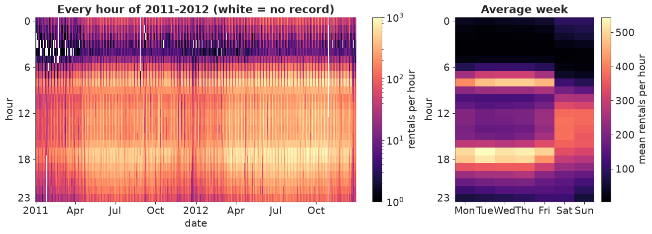
Two regimes jump out: workdays have two commuter spikes (8 am, 5-6 pm), weekends one broad afternoon hump; 2012 is visibly brighter than 2011 (the system was growing), summers brighter than winters, and the white vertical stripes are the gaps listed above.

2 · A modest model with named dimensions

The model is a vehicle, so it is kept small. Rentals in hour $h$ of date $d$:

$$ \begin{aligned} y_{dh} &\sim \text{NegBinomial}(\mu_{dh}, \alpha) \\ \log \mu_{dh} &= a_{k} + \text{profile}_{k,h} + \beta_{k} T_{dh} + \gamma_{k} T_{dh}^2 + w_{\text{weather}_{dh}} + \tau \, t_d \end{aligned} $$

where $k$ is the day type (workday or off day), $T = (\text{temp} - 15\,°C)/10$, $w$ is a sum-to-zero weather effect and $t_d$ is time in years (the system grew). The hour-of-day profile is a ZeroSumNormal over hours within each day type.

The data are a date x hour grid with holes; the likelihood wants a flat list of recorded hours. stack makes the rows (a MultiIndex of (date, hour)) and dropna removes the holes. Every covariate, including the day-level coords, comes along for free.

rows = ds.stack(obs=("date", "hour")).dropna("obs", subset=["cnt"])
print(rows.sizes, rows.indexes["obs"][:3].tolist(), sep="\n")

DAYTYPES = ["workday", "off day"]
daytype_idx = pd.Index(DAYTYPES).get_indexer(rows.daytype.values)
weather_idx = pd.Index(WEATHER).get_indexer(rows.weather.values)
assert (daytype_idx >= 0).all() and (weather_idx >= 0).all()

coords = {
    "daytype": DAYTYPES, "hour": np.arange(24), "weather": WEATHER,
    "obs": np.arange(rows.sizes["obs"]),
}
T_rows = (rows.temp_c.values - 15) / 10

with pm.Model(coords=coords) as model:
    a = pm.Normal("a", 5, 1.5, dims="daytype")
    profile = pm.ZeroSumNormal("profile", sigma=1.5, dims=("daytype", "hour"), n_zerosum_axes=1)
    b_temp = pm.Normal("b_temp", 0, 0.5, dims="daytype")
    b_temp2 = pm.Normal("b_temp2", 0, 0.5, dims="daytype")
    weather_eff = pm.ZeroSumNormal("weather_eff", sigma=0.5, dims="weather")
    trend = pm.Normal("trend", 0, 0.5)
    alpha = pm.Gamma("alpha", 2, 0.2)

    eta = (
        a[daytype_idx] + profile[daytype_idx, rows.hour.values]
        + b_temp[daytype_idx] * T_rows + b_temp2[daytype_idx] * T_rows**2
        + weather_eff[weather_idx] + trend * rows.t_years.values
    )
    pm.NegativeBinomial(
        "cnt", mu=pm.math.exp(eta), alpha=alpha, observed=rows.cnt.values.astype(int), dims="obs"
    )

model

Frozen({'obs': 17379})
[(Timestamp('2011-01-01 00:00:00'), 0), (Timestamp('2011-01-01 00:00:00'), 1), (Timestamp('2011-01-01 00:00:00'), 2)]

$$ \begin{array}{rcl} \text{a} &\sim & \operatorname{Normal}(5,~1.5)\\\text{profile} &\sim & \operatorname{ZeroSumNormal}(1.5,~\text{<constant>})\\\text{b_temp} &\sim & \operatorname{Normal}(0,~0.5)\\\text{b_temp2} &\sim & \operatorname{Normal}(0,~0.5)\\\text{weather_eff} &\sim & \operatorname{ZeroSumNormal}(0.5,~\text{<constant>})\\\text{trend} &\sim & \operatorname{Normal}(0,~0.5)\\\text{alpha} &\sim & \operatorname{Gamma}(2,~\text{<constant>})\\\text{cnt} &\sim & \operatorname{NegativeBinomial}(\text{alpha},~f(\text{alpha},~\text{trend},~\text{weather_eff},~\text{b_temp2},~\text{b_temp},~\text{profile},~\text{a})) \end{array} $$

Priors: a ~ Normal(5, 1.5) puts the baseline between roughly 10 and 3000 rentals an hour; a 10 °C change multiplying rentals by more than $e^{1} \approx 2.7$ is already unlikely under Normal(0, 0.5). With 17k rows the likelihood dominates all of these; we skip the prior predictive check here (E01 shows it) and go straight to sampling.

with model:
    idata = pm.sample(random_seed=RANDOM_SEED)

summ = az.summary(idata, round_to=4)
print(
    f"nutpie, {idata.posterior.attrs['tuning_steps']} tuning steps; "
    f"max r_hat {summ.r_hat.max():.3f}, min bulk ESS {summ.ess_bulk.min():.0f}, "
    f"min tail ESS {summ.ess_tail.min():.0f}, "
    f"divergences {int(idata.sample_stats['diverging'].sum())}"
)
az.summary(idata, var_names=["a", "b_temp", "b_temp2", "weather_eff", "trend", "alpha"],
           round_to=3)

nutpie, 400 tuning steps; max r_hat 1.006, min bulk ESS 915, min tail ESS 1578, divergences 0

	mean	sd	eti89_lb	eti89_ub	ess_bulk	ess_tail	r_hat	mcse_mean	mcse_sd
a[workday]	4.081	0.007	4.069	4.093	915.453	1577.902	1.005	0.000	0.000
a[off day]	4.181	0.009	4.166	4.195	1193.670	1712.584	1.006	0.000	0.000
b_temp[workday]	0.318	0.004	0.311	0.324	5176.097	3269.444	1.000	0.000	0.000
b_temp[off day]	0.421	0.005	0.412	0.430	5245.245	2776.211	1.001	0.000	0.000
b_temp2[workday]	-0.127	0.004	-0.133	-0.120	2530.283	2431.321	1.002	0.000	0.000
b_temp2[off day]	-0.175	0.006	-0.184	-0.166	2919.273	2759.055	1.000	0.000	0.000
weather_eff[clear]	0.229	0.004	0.222	0.236	2471.431	2589.775	1.002	0.000	0.000
weather_eff[mist]	0.128	0.005	0.121	0.136	3442.856	3187.043	1.001	0.000	0.000
weather_eff[rain/snow]	-0.357	0.007	-0.368	-0.347	1931.578	2580.384	1.003	0.000	0.000
trend	0.435	0.005	0.427	0.443	1085.557	1858.918	1.003	0.000	0.000
alpha	9.719	0.123	9.522	9.917	5892.101	3101.951	1.001	0.002	0.002

Clean: all r_hat at 1.00-1.01, at least ~900 effective draws, no divergences. The trend of about 0.44 per year means rentals grew by a factor of $e^{0.44} \approx 1.55$ a year at fixed weather and temperature. The rest of the notebook is about using this posterior.

3 · The `DataTree`: groups, names and the sample dimension

pm.sample returns an xr.DataTree. Each child is a Dataset whose variables share the chain and draw dimensions plus the model's own dims.

print(list(idata.children))
idata.posterior

['posterior', 'sample_stats', 'constant_data', 'observed_data']

The one before/after in this notebook. The positional way needs you to remember the axis order (chain, draw, daytype, hour) and which integer means "workday". Add a dimension to the model next month (say year) and the first line silently computes something else; the second keeps meaning what it says.

prof = idata.posterior["profile"]
positional = prof.values[:, :, 0, 8].mean()  # before: which axis is which? is 0 "workday"?
named = prof.sel(daytype="workday", hour=8).mean(("chain", "draw"))  # after
print(f"{positional:.4f} == {float(named):.4f}")

1.5982 == 1.5982

Operations on the tree apply to every group that has the dimension. Thinning with isel thins posterior and sample_stats together (keeping the draw labels, so draw 10 is still draw 10), and leaves observed_data alone.

thin = idata.isel(draw=slice(None, None, 10))
for name, node in thin.children.items():
    print(f"{name:14s}", dict(node.sizes))
print("kept draw labels:", thin.posterior.draw.values[:5])

posterior      {'chain': 4, 'draw': 100, 'daytype': 2, 'hour': 24, 'weather': 3}
sample_stats   {'chain': 4, 'draw': 100}
constant_data  {}
observed_data  {'obs': 17379}
kept draw labels: [ 0 10 20 30 40]

Most summaries do not care which chain a draw came from. az.extract stacks chain and draw into one sample dimension (a MultiIndex, so nothing is lost) and returns a plain Dataset; .unstack("sample") goes back. We will use post for all posterior arithmetic.

post = az.extract(idata)
print(dict(post.sizes))
print(post.indexes["sample"][:3].tolist())
print("unstacked:", post["profile"].unstack("sample").dims)

{'daytype': 2, 'sample': 4000, 'hour': 24, 'weather': 3}
[(0, 0), (0, 1), (0, 2)]
unstacked: ('daytype', 'hour', 'chain', 'draw')

And when a tidy-data tool is the right one, to_dataframe() gives one row per labelled cell with the dims as the index. Here: the multiplicative weather effects relative to the average weather, as a small table.

tidy = np.exp(idata.posterior["weather_eff"]).to_dataframe().reset_index()
print(tidy.head(3))
tidy.groupby("weather")["weather_eff"].quantile([0.05, 0.5, 0.95]).unstack().round(3)

   chain  draw    weather  weather_eff
0      0     0      clear     1.263241
1      0     0       mist     1.139122
2      0     0  rain/snow     0.694934

	0.05	0.50	0.95
weather
clear	1.249	1.257	1.266
mist	1.128	1.137	1.146
rain/snow	0.692	0.700	0.707

Posterior predictive draws, back on the calendar

sample_posterior_predictive returns draws on the model's flat obs dimension. We saved the MultiIndex of those rows when we stacked, so putting the draws back on the date x hour grid is assign_coords + unstack. We use the thinned tree (400 draws): 17k rows x 4000 draws would be 560 MB of integers, and 400 draws are plenty for predictive summaries.

with model:
    pp = pm.sample_posterior_predictive(thin, random_seed=RANDOM_SEED)

obs_mi = xr.Coordinates.from_pandas_multiindex(rows.indexes["obs"], "obs")
yrep = (
    pp.posterior_predictive["cnt"]
    .assign_coords(obs_mi)  # obs: 0..17378  ->  obs: (date, hour)
    .unstack("obs")  # -> (chain, draw, date, hour), NaN where no record
    .stack(sample=("chain", "draw"))
    .transpose("sample", "date", "hour")
    .assign_coords({k: ds[k] for k in ["weekday", "workingday", "holiday", "daytype"]})
)
del pp
yrep

yrep has NaN exactly where the data have no record, so any comparison of yrep with ds.cnt is automatically like with like.

4 · Broadcasting by name: counterfactual grids without loops

A planner asks: how many bikes will be taken each hour on a clear day, as a function of temperature, on a workday versus an off day? The posterior mean function is a formula in the parameters; to evaluate it on a grid we make the grid a set of named arrays and write the formula. xarray aligns dimensions by name and broadcasts the rest: a has (daytype, sample), profile has (daytype, hour, sample), the temperature grid has (temp_c,), and the result has all four. No reshape, no np.newaxis, no loop.

temp_grid = xr.DataArray(np.arange(-5.0, 36.0), dims="temp_c", name="temp_c")
temp_grid = temp_grid.assign_coords(temp_c=temp_grid)
T = (temp_grid - 15) / 10
t_mid2012 = 1.5  # years since 2011-01-01: fix the growth trend at mid-2012

log_mu = (
    post["a"] + post["profile"] + post["b_temp"] * T + post["b_temp2"] * T**2
    + post["weather_eff"].sel(weather="clear", drop=True) + post["trend"] * t_mid2012
)
mu = np.exp(log_mu).rename("mu")
print(mu.dims, f"{mu.nbytes / 1e6:.0f} MB")

('daytype', 'sample', 'hour', 'temp_c') 63 MB

mu is 63 MB of posterior mean functions: one for each of the 4000 draws at each of 2 x 24 x 41 grid points. Its posterior mean is a two-panel heatmap straight from xarray's FacetGrid (col="daytype").

fg = mu.mean("sample").plot(
    x="temp_c", y="hour", col="daytype", cmap="magma", yincrease=False, size=4, aspect=1.2,
    cbar_kwargs={"label": "expected rentals per hour (clear, mid-2012)"},
)
fg.set_axis_labels("temperature (°C)", "hour of day")
fg.set_titles("{value}");

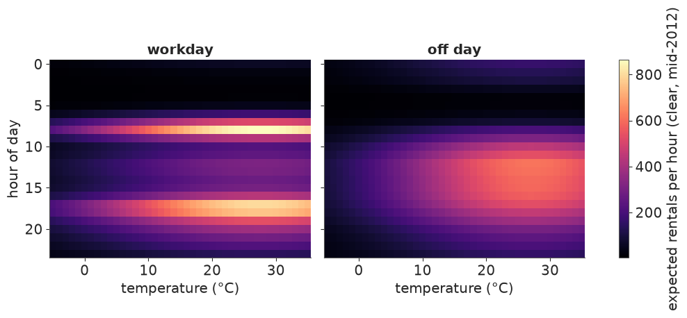
Workdays are a two-spike day at every temperature; off days one broad afternoon block that lights up more strongly with warmth. Both peak around 27 °C and ease off above that (the quadratic term). This is the model's view of mid-2012 on a clear day; any other scenario is one .sel or one number away.

Contrasts are subtraction of selections. Workday minus off day leaves (hour, temp_c, sample); we pick three temperatures and summarise over sample with .quantile, which adds a quantile dimension we can select from when plotting.

contrast = mu.sel(daytype="workday") - mu.sel(daytype="off day")
c_q = contrast.sel(temp_c=[5.0, 20.0, 30.0]).quantile([0.03, 0.5, 0.97], dim="sample")

fig, ax = plt.subplots(figsize=(9, 3.8))
for temp_c, color in zip(c_q.temp_c.values, ["#6ba4e8", BLUE, ORANGE]):
    q = c_q.sel(temp_c=temp_c)
    ax.fill_between(q.hour, q.sel(quantile=0.03), q.sel(quantile=0.97), color=color, alpha=0.3)
    ax.plot(q.hour, q.sel(quantile=0.5), color=color, label=f"{temp_c:.0f} °C")
ax.axhline(0, color=GREY, lw=0.8)
ax.set(xlabel="hour of day", ylabel="workday minus off day\n(expected rentals per hour)",
       xticks=range(0, 24, 2), title="Where the workday gains and loses riders")
ax.legend(title="temperature");

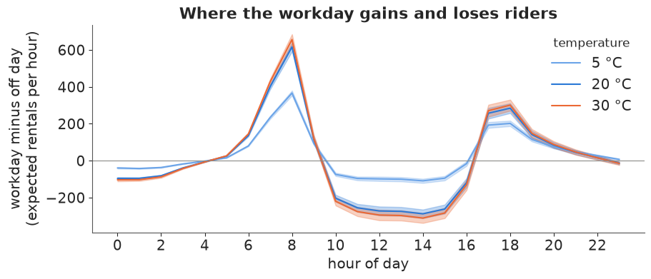
At 20-30 °C a workday adds about 600 riders at 8 am and about 300 at 5-6 pm, and loses 200-300 an hour from 10 am to 3 pm (a warm weekend afternoon is the leisure peak). At 5 °C every one of those differences shrinks, because cold scales all hours down together. The 94% bands are barely wider than the lines: with 17k hourly counts, the mean function is pinned down tightly. The uncertainty that matters to a planner is predictive - how many bikes will actually be taken - which is next.

A predictive clock: lifting a NumPy RNG with `apply_ufunc`

numpy.random.Generator.negative_binomial knows nothing about names, but xr.apply_ufunc will broadcast its labelled inputs by name, call the function on the aligned arrays and put the labels back on. That gives predictive draws on the grid with one call (using the NegBinomial's n = alpha, p = alpha / (alpha + mu) parameterisation).

mu20 = mu.sel(temp_c=20.0)
ytilde = xr.apply_ufunc(
    rng.negative_binomial, post["alpha"], post["alpha"] / (post["alpha"] + mu20)
).rename("rentals")
bands = ytilde.quantile([0.05, 0.25, 0.5, 0.75, 0.95], dim="sample")
print(ytilde.dims)
print("workday 5 pm, 20 °C:", bands.sel(daytype="workday", hour=17).round().values)

('sample', 'daytype', 'hour')
workday 5 pm, 20 °C: [ 398.  572.  718.  889. 1177.]

theta = 2 * np.pi * (np.arange(25) % 24) / 24  # close the circle: hour 0 again at the end

fig, axes = plt.subplots(1, 2, figsize=(11, 5.4), subplot_kw={"projection": "polar"})
for ax, daytype, color in zip(axes, DAYTYPES, [BLUE, ORANGE]):
    b = bands.sel(daytype=daytype).isel(hour=np.arange(25) % 24)
    ax.fill_between(theta, b.sel(quantile=0.05), b.sel(quantile=0.95), color=color, alpha=0.2,
                    label="90% of hours")
    ax.fill_between(theta, b.sel(quantile=0.25), b.sel(quantile=0.75), color=color, alpha=0.45,
                    label="50% of hours")
    ax.plot(theta, mu20.sel(daytype=daytype).mean("sample").isel(hour=np.arange(25) % 24),
            color=color, lw=2, label="expected")
    ax.set_theta_zero_location("N")
    ax.set_theta_direction(-1)
    ax.set_xticks(2 * np.pi * np.arange(0, 24, 3) / 24, [f"{h}h" for h in range(0, 24, 3)])
    ax.set_rlim(0, 1.02 * float(bands.max()))
    ax.set_rticks([300, 600, 900], ["300", "600", "900"], fontsize=8)
    ax.set_rlabel_position(100)
    ax.set_title(f"{daytype}, clear, 20 °C", pad=18)
fig.legend(*axes[1].get_legend_handles_labels(), loc="outside lower center", ncols=3);

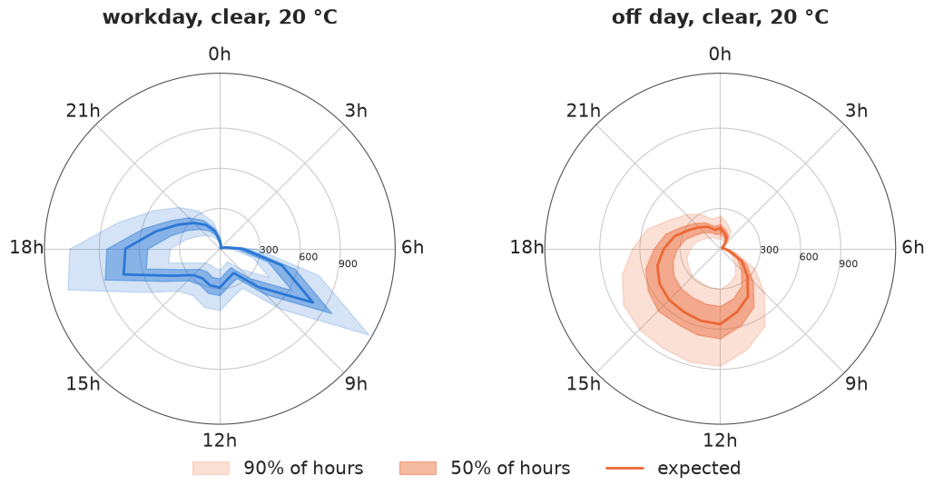
Read it like a clock face: midnight at the top, noon at the bottom. The workday clock has two lobes pointing at 8 am and 5-6 pm; the off-day clock one fat lobe over the afternoon. The bands are hours, not parameters: at 5 pm on a clear 20 °C workday the median is about 720 rentals, half of such hours see 570-890 and one in ten falls outside 400-1180. That spread is the NegBinomial overdispersion; the posterior of the mean is a thin line inside it. (Section 6 will show this single overdispersion parameter is standing in for something else.)

5 · Time machinery on posterior predictive draws

Planners want totals: per week, per month, per season. The rule that makes this correct: aggregate the draws, then summarise. A quantile of a sum is not the sum of quantiles. Because every draw is a complete replicated history, yrep.sum("hour") is a posterior predictive draw of daily totals, and every time operation xarray has works on it.

First, daily totals and a demonstration of the rule with weekly totals via resample.

obs_day = ds.cnt.sum("hour")  # missing hours count as 0 in both: like for like
rep_day = yrep.sum("hour")

rep_week = rep_day.resample(date="W").sum()  # weekly totals, per draw
right = rep_week.quantile([0.05, 0.95], dim="sample")
wrong = rep_day.quantile([0.05, 0.95], dim="sample").resample(date="W").sum()
width = lambda q: q.sel(quantile=0.95) - q.sel(quantile=0.05)  # noqa: E731
print(f"weeks: {rep_week.sizes['date']}, labelled by the Sunday that ends them:",
      rep_week.date.values[:2].astype("datetime64[D]"))
print(f"median 90% width, draws summed first:      {float(width(right).median()):,.0f}")
print(f"median 90% width, daily quantiles summed:  {float(width(wrong).median()):,.0f}  (wrong)")

weeks: 106, labelled by the Sunday that ends them:

 ['2011-01-02' '2011-01-09']
median 90% width, draws summed first:      3,301
median 90% width, daily quantiles summed:  8,510  (wrong)

Summing daily quantiles gives intervals several times too wide: it assumes every day of the week is simultaneously at its own 5th percentile, which the model says almost never happens. Aggregating draws keeps whatever dependence the model has between days - here, given the parameters, days are independent, so the errors partly cancel. Whether days really are independent is a modelling claim, and section 6 checks it.

coarsen is the index-agnostic cousin of resample: fixed blocks of 7 rows starting at the first date (a Saturday), labelled by the block's centre date. Different weeks, same totals-per-block logic - choose resample when the calendar matters. One trap: coarsen also averages every non-dimension coordinate along date (coord_func="mean"), which raises a TypeError on string coords such as weekday, so drop (or give a coord_func for) them.

blocks = obs_day.drop_vars(["weekday", "daytype"]).coarsen(date=7, boundary="trim").sum()
print("coarsen labels:", blocks.date.values[:2].astype("datetime64[D]"),
      "| resample labels:", rep_week.date.values[:2].astype("datetime64[D]"))

coarsen labels: ['2011-01-04' '2011-01-11'] | resample labels: ['2011-01-02' '2011-01-09']

A fan chart of monthly totals, and a rolling view

resample(date="MS") gives monthly totals per draw; .quantile with five levels gives a quantile dimension, i.e. a fan. On the right, a 7-day centred rolling mean, again per draw first, for 2012.

rep_month = rep_day.resample(date="MS").sum()
obs_month = obs_day.resample(date="MS").sum()
fan = rep_month.quantile([0.05, 0.25, 0.5, 0.75, 0.95], dim="sample")

rep_roll = rep_day.sel(date="2012").rolling(date=7, center=True).mean()
obs_roll = obs_day.sel(date="2012").rolling(date=7, center=True).mean()
roll_q = rep_roll.quantile([0.05, 0.95], dim="sample")

fig, axes = plt.subplots(1, 2, figsize=(13, 4.2), width_ratios=[1, 1.3])
ax = axes[0]
x = fan.date.values
ax.fill_between(x, fan.sel(quantile=0.05), fan.sel(quantile=0.95), color=BLUE, alpha=0.2,
                step="mid", label="90%")
ax.fill_between(x, fan.sel(quantile=0.25), fan.sel(quantile=0.75), color=BLUE, alpha=0.45,
                step="mid", label="50%")
ax.plot(x, fan.sel(quantile=0.5), color=BLUE, drawstyle="steps-mid", lw=1)
ax.plot(x, obs_month, "o", color="k", ms=4, label="observed")
ax.set(ylabel="rentals per month", title="Monthly totals: posterior predictive fan")
ax.xaxis.set_major_locator(mdates.MonthLocator(bymonth=[1, 7]))
ax.xaxis.set_major_formatter(mdates.DateFormatter("%b\n%Y"))
ax.legend(loc="upper left")

ax = axes[1]
ax.fill_between(roll_q.date, roll_q.sel(quantile=0.05), roll_q.sel(quantile=0.95), color=BLUE,
                alpha=0.3, label="replicated, 90%")
ax.plot(obs_roll.date, obs_roll, color="k", lw=1.2, label="observed")
ax.set(ylabel="rentals per day (7-day mean)", title="2012, 7-day rolling mean")
ax.xaxis.set_major_formatter(mdates.DateFormatter("%b"))
ax.legend(loc="upper left");

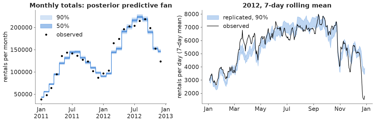
The xarray part worked; the model did not pass this check. The monthly bands are only a few percent wide, yet most observed months fall outside them: spring (April-June 2011, March-April 2012) runs well above the fan and December 2012 far below it. The rolling view says why: the observed line leaves the band for weeks at a time - a warm-weather surge in March 2012, the Sandy shutdown at the end of October, the Christmas collapse. Errors that persist over days cannot cancel when we sum days, so aggregating the draws of a model without them gives confidently wrong totals. Keep that in mind through section 6.

`groupby("date.month")`, `cumulative` and `.where`

The virtual coordinate "date.month" groups by calendar month across both years. Here we compute, per draw, how far the observed monthly mean sits from the replicated one, as a ratio. This is a posterior distribution of the model's error for each calendar month.

ratio = obs_day.groupby("date.month").mean() / rep_day.groupby("date.month").mean()
ratio.quantile([0.05, 0.5, 0.95], dim="sample").to_pandas().T.round(3)

quantile	0.05	0.50	0.95
month
1	0.984	1.006	1.028
2	0.969	0.991	1.013
3	1.031	1.053	1.073
4	1.065	1.088	1.109
5	1.047	1.069	1.087
6	1.022	1.041	1.061
7	0.937	0.956	0.977
8	0.934	0.951	0.970
9	0.968	0.988	1.007
10	1.016	1.034	1.054
11	0.949	0.970	0.989
12	0.843	0.862	0.880

Observed daily rentals run 4-9% above the model from March to June and 4-5% below it in July-August, and December sits 14% below; most intervals exclude 1. Seasonality enters this model only through temperature, so "spring enthusiasm" at a given temperature and the holiday lull are invisible to it.

cumulative("date").sum() is a running total (the modern spelling of cumsum, with the same API as rolling). Per draw, "the first date the 2012 running total reaches one million" is (running >= 1e6).idxmax("date"): a posterior predictive distribution over a date.

running = rep_day.sel(date="2012").cumulative("date").sum()
millionth = (running >= 1e6).idxmax("date")
obs_millionth = (obs_day.sel(date="2012").cumulative("date").sum() >= 1e6).idxmax("date")
print("observed:", obs_millionth.values.astype("datetime64[D]"))
print("replicated 5/50/95%:",
      pd.to_datetime(millionth.values).to_series().quantile([0.05, 0.5, 0.95]).dt.date.tolist())

observed: 2012-07-11
replicated 5/50/95%: [datetime.date(2012, 7, 17), datetime.date(2012, 7, 18), datetime.date(2012, 7, 20)]

.where keeps the shape and masks with NaN, so it combines with coords to carve out a sub-population without losing alignment. What share of workday rentals happen in the four commuter hours (7-8 am, 5-6 pm)? Per draw, then summarised:

commute = yrep.hour.isin([7, 8, 17, 18]) & (yrep.workingday == 1)
share_rep = yrep.where(commute).sum(("date", "hour")) / yrep.where(yrep.workingday == 1).sum(
    ("date", "hour"))
share_obs = ds.cnt.where(commute).sum() / ds.cnt.where(ds.workingday == 1).sum()
print(f"observed commuter share {float(share_obs):.3f}; replicated 90% interval "
      f"{float(share_rep.quantile(0.05)):.3f}-{float(share_rep.quantile(0.95)):.3f}")

observed commuter share 0.387; replicated 90% interval 0.386-0.396

6 · Calibration by bins: where does the model get it wrong?

Per recorded hour we compute three diagnostics from the 400 replicated draws, all as labelled date x hour arrays:

the (mid-)PIT, $P(y^{rep} < y) + \tfrac12 P(y^{rep} = y)$: uniform if calibrated;
a standardised residual $z = (y - \bar y^{rep}) / \text{sd}(y^{rep})$;
whether $y$ falls inside the central 90% predictive interval.

y = ds.cnt
pit = ((yrep < y).mean("sample") + 0.5 * (yrep == y).mean("sample")).where(y.notnull())
z = (y - yrep.mean("sample")) / yrep.std("sample")
q05, q95 = yrep.quantile(0.05, dim="sample"), yrep.quantile(0.95, dim="sample")
inside = ((y >= q05) & (y <= q95)).where(y.notnull())

diag = xr.Dataset({"pit": pit, "z": z, "inside90": inside}).assign_coords(
    temp_c=ds.temp_c, weather=ds.weather
)
print(f"overall 90% coverage: {float(diag.inside90.mean()):.3f}")

overall 90% coverage: 0.910

Binning on a 2-D coordinate. temp_c varies over both date and hour; groupby with a BinGrouper flattens whatever it needs to. groupby_bins is the older spelling of the same thing. The multi-key form takes one grouper per coordinate and returns a grid: here hour-of-day blocks (a BinGrouper on the hour dimension, with labels) by weather.

temp_bins = np.arange(-10, 45, 5)
by_temp = diag.groupby(temp_c=BinGrouper(bins=temp_bins)).mean()
n_temp = diag.pit.groupby(temp_c=BinGrouper(bins=temp_bins)).count()
same = diag.z.groupby_bins("temp_c", bins=temp_bins).mean()
assert np.allclose(same.values, by_temp.z.values, equal_nan=True)

hour_blocks = BinGrouper(
    bins=[-1, 5, 9, 15, 19, 23],
    labels=["night 0-5", "am rush 6-9", "midday 10-15", "pm rush 16-19", "evening 20-23"],
)
grid = diag.groupby(hour=hour_blocks, weather=UniqueGrouper()).mean().sel(weather=WEATHER)
grid.z.to_pandas().round(2)

weather	clear	mist	rain/snow
hour_bins
night 0-5	-0.02	-0.03	0.42
am rush 6-9	0.03	-0.05	-0.11
midday 10-15	-0.02	0.09	-0.22
pm rush 16-19	-0.01	-0.02	0.10
evening 20-23	0.03	-0.07	-0.09

fig, axes = plt.subplots(1, 3, figsize=(14, 4), width_ratios=[1, 1.2, 1.2])
ax = axes[0]
ax.hist(diag.pit.values.ravel(), bins=20, range=(0, 1), color=BLUE, alpha=0.8, density=True)
ax.axhline(1, color="k", lw=1, ls="--")
ax.set(xlabel="PIT", ylabel="density", title="Hourly PIT (flat = calibrated)")

ax = axes[1]
mids = [iv.mid for iv in by_temp.temp_c_bins.values]
ax.bar(mids, by_temp.inside90, width=4, color=BLUE, alpha=0.8)
ax.axhline(0.9, color="k", ls="--", lw=1)
for m, v, n in zip(mids, by_temp.inside90.values, n_temp.values):
    ax.text(m, v + 0.01, f"{n}", ha="center", fontsize=7, color=GREY)
ax.set(xlabel="temperature bin (°C)", ylabel="share inside 90% interval", ylim=(0, 1.05),
       title="Coverage by temperature (n hours)")

ax = axes[2]
lim = float(np.abs(grid.z).max())
im = ax.imshow(grid.z.transpose("weather", "hour_bins"), cmap="RdBu_r", vmin=-lim, vmax=lim,
               aspect="auto")
ax.set_xticks(range(5), [s.replace(" ", "\n", 1) for s in grid.hour_bins.values], fontsize=8)
ax.set_yticks(range(3), WEATHER)
for (i, j), v in np.ndenumerate(grid.z.transpose("weather", "hour_bins").values):
    ax.text(j, i, f"{v:+.2f}", ha="center", va="center", fontsize=8)
ax.set_title("Mean standardised residual")
fig.colorbar(im, ax=ax, label="z (observed above model > 0)");

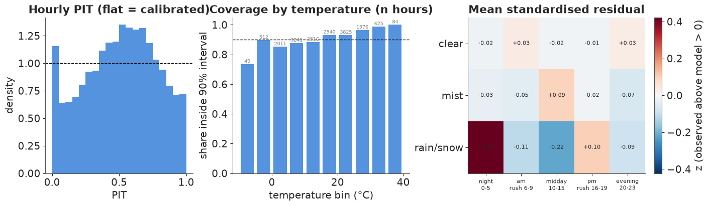
Three readings, each from one line of grouping code:

Hourly PIT is far from flat: a hump in the middle (for typical hours the predictive distribution is too wide) plus a spike at 0 (hours with far fewer riders than expected). Both are what a missing day-level effect does: good days and bad days are pooled into one overdispersion parameter, which then over-covers ordinary hours and still misses bad days.
Coverage by temperature: the overall 91% hides a slope, from 74-88% below 15 °C (the few hours below -5 °C are the worst) to 96-100% above 25 °C.
Hour block x weather: clear and misty hours are fine (|z| < 0.1). Rain costs more riders at midday (z = -0.22) than the single multiplicative weather effect allows, and fewer at night (+0.42): the weather effect should depend on the hour.

The week as a heatmap: the mean, the uncertainty, and the surprise

Three weekday x hour summaries from one groupby("weekday") on a Dataset of three derived variables: what the model expects, how uncertain a single hour is (the predictive coefficient of variation, sd / mean), and where the data disagree (mean z).

week = (
    xr.Dataset({"expected": yrep.mean("sample"), "cv": yrep.std("sample") / yrep.mean("sample"),
                "z": diag.z})
    .groupby("weekday").mean()
    .pipe(numeric_weekday)
)
fig, axes = plt.subplots(1, 3, figsize=(14, 4.6), sharey=True)
week.expected.plot(x="weekday", y="hour", ax=axes[0], cmap="magma", yincrease=False,
                   cbar_kwargs={"label": "expected rentals"})
week.cv.plot(x="weekday", y="hour", ax=axes[1], cmap="viridis", yincrease=False,
             cbar_kwargs={"label": "predictive sd / mean"})
week.z.plot(x="weekday", y="hour", ax=axes[2], cmap="RdBu_r", center=0, yincrease=False,
            cbar_kwargs={"label": "mean z (observed above model > 0)"})
for ax, title in zip(axes, ["What the model expects", "How uncertain an hour is",
                            "Where the data disagree"]):
    ax.set(title=title, xlabel="", ylabel="")
    ax.set_xticks(range(7), DOW)
axes[0].set_ylabel("hour of day");

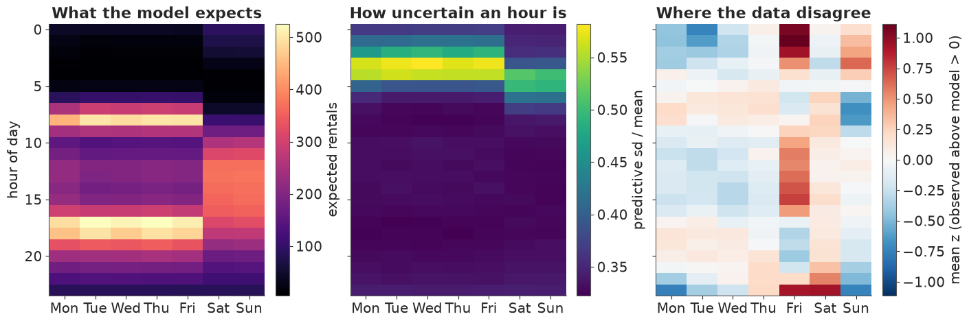
The middle panel explains a NegBinomial fact: the predictive coefficient of variation is about $\sqrt{1/\mu + 1/\alpha}$, so it is largest at 3-5 am when counts are tiny, and flattens out near $1/\sqrt{\alpha} \approx 0.32$ whenever the counts are large. The right panel is the interesting one: Friday is not an ordinary workday (more riders from late morning to mid-afternoon, fewer in the evening rush), the small hours of Friday and Sunday and late Saturday evening are busier than the profiles say, and Sunday morning and the last hours of Sunday and Monday are quieter. Two day types are too few; a weekday x hour profile is the obvious next model, and it would drop into the same code.

A calendar of surprise

Finally, one PIT per day from the daily totals: near 0 means far fewer rentals than the model expected for that date's weather and calendar, near 1 far more. To draw it as a calendar we give each date a (year, week-of-year, weekday) label and reshape by those labels: set_index(date=[...]) turns them into a MultiIndex and unstack spreads it into three dimensions. (ISO week numbers do not work here: 1 January 2011 is in ISO week 52 of 2010, so (year, week, weekday) would repeat and unstack refuses duplicates.)

pit_day = (rep_day < obs_day).mean("sample") + 0.5 * (rep_day == obs_day).mean("sample")
d = pit_day.indexes["date"]
jan1 = pd.to_datetime(d.year.astype(str) + "-01-01")
cal = (
    pit_day.assign_coords(
        year=("date", d.year), dow=("date", d.dayofweek),
        week=("date", (d.dayofyear - 1 + jan1.dayofweek) // 7),
    )
    .drop_vars(["weekday", "workingday", "holiday", "daytype"])
    .set_index(date=["year", "week", "dow"])
    .unstack("date")
)
print(dict(cal.sizes))

fg = cal.plot(x="week", y="dow", row="year", cmap="RdBu_r", vmin=0, vmax=1, yincrease=False,
              size=2.1, aspect=5.5, cbar_kwargs={"label": "daily PIT", "shrink": 0.8})
for ax in fg.axs.flat:
    ax.set_yticks(range(7), DOW, fontsize=7)
    ax.set_xticks(np.arange(0, 53, 4.35), ["Jan", "Feb", "Mar", "Apr", "May", "Jun", "Jul",
                                            "Aug", "Sep", "Oct", "Nov", "Dec", ""], fontsize=8)
    ax.set_xlabel("")
fg.set_titles("{value}");

{'year': 2, 'week': 54, 'dow': 7}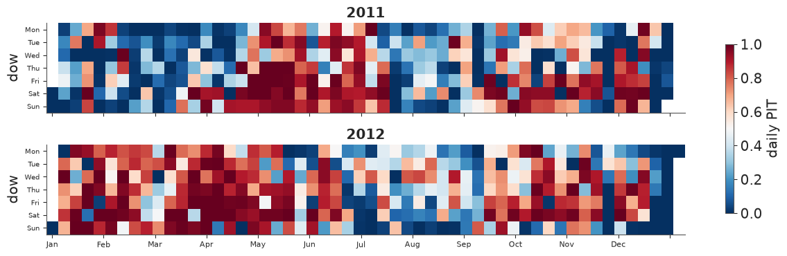

If the model were calibrated at the daily level this would be salt-and-pepper noise with 10% of the days deep red or deep blue. Instead a third of all days fall outside their 90% interval, and the colours come in runs: blue in January-February and July-August 2011, red through the first five months of 2012, blue again in its summer, dark blue over both Christmas weeks. A shock shared by all the hours of a day - and often by neighbouring days - is exactly what the hourly model lacks.

.where(..., drop=True) pulls out the most surprising days as a short list, keeping their coords (weekday, holiday) attached:

outside = (pit_day < 0.05) | (pit_day > 0.95)
print(f"days outside the 90% predictive interval: {float(outside.mean()):.0%} (should be 10%)")

ratio_day = (obs_day / rep_day.mean("sample")).rename("observed / expected")
surprise = ratio_day.where((ratio_day < 0.5) | (ratio_day > 1.5), drop=True)
surprise.to_dataframe()[["weekday", "holiday", "observed / expected"]].round(2)

days outside the 90% predictive interval: 34% (should be 10%)

	weekday	holiday	observed / expected
date
2011-01-01	Sat	0	0.46
2011-01-02	Sun	0	0.46
2011-03-06	Sun	0	0.33
2011-03-10	Thu	0	0.35
2011-04-16	Sat	0	0.38
2011-04-30	Sat	0	1.50
2011-08-27	Sat	0	0.45
2011-10-29	Sat	0	0.48
2011-11-24	Thu	1	0.40
2011-12-07	Wed	0	0.31
2011-12-24	Sat	0	0.36
2011-12-25	Sun	0	0.27
2011-12-26	Mon	1	0.43
2011-12-27	Tue	0	0.40
2012-04-22	Sun	0	0.43
2012-11-22	Thu	1	0.45
2012-12-22	Sat	0	0.44
2012-12-23	Sun	0	0.45
2012-12-24	Mon	0	0.29
2012-12-25	Tue	1	0.24
2012-12-26	Wed	0	0.17
2012-12-27	Thu	0	0.49
2012-12-29	Sat	0	0.45
2012-12-30	Sun	0	0.48

The biggest misses are recognisable: the Christmas-New Year weeks, Thanksgiving (24 November 2011, 22 November 2012), 1-2 January 2011 and 27 August 2011 as Hurricane Irene arrived. Hurricane Sandy (29-30 October 2012) is not on the list: the hours when the system was shut have no record, and yrep is masked at exactly the same hours, so the daily totals compare like with like. That is a choice to be aware of - a masked comparison cannot see an outage.

7 · Fixing the day-level misfit, and predicting new days by broadcasting

The calendar says the missing piece is a shock shared by all hours of a day (a holiday week, a storm the hourly weather code under-rates, an event in town). The smallest fix is a day-level effect. We write it hierarchically centred: each date gets a level whose mean is the day-level part of the old predictor,

$$ \ell_d \sim \text{Normal}(a_{k(d)} + \tau t_d,\ \sigma_{\text{day}}), \qquad \log \mu_{dh} = \ell_d + \text{profile}_{k,h} + \beta_k T_{dh} + \gamma_k T_{dh}^2 + w_{\text{weather}_{dh}} $$

A zero-mean day effect added to $a + \tau t$ gave a ridge between the intercept, the trend and the 731 day effects (min bulk ESS about 170, r_hat 1.02-1.03, even with 1000 tuning steps or a sum-to-zero day effect); centring the level on them removes the ridge. The model gets one new dimension, date, and its coordinate is the actual DatetimeIndex.

date_idx = ds.indexes["date"].get_indexer(rows.date.values)
daytype_of_date = pd.Index(DAYTYPES).get_indexer(ds.daytype.values)

with pm.Model(coords=coords | {"date": ds.indexes["date"]}) as model_day:
    a = pm.Normal("a", 5, 1.5, dims="daytype")
    profile = pm.ZeroSumNormal("profile", sigma=1.5, dims=("daytype", "hour"), n_zerosum_axes=1)
    b_temp = pm.Normal("b_temp", 0, 0.5, dims="daytype")
    b_temp2 = pm.Normal("b_temp2", 0, 0.5, dims="daytype")
    weather_eff = pm.ZeroSumNormal("weather_eff", sigma=0.5, dims="weather")
    trend = pm.Normal("trend", 0, 0.5)
    alpha = pm.Gamma("alpha", 2, 0.2)
    sigma_day = pm.HalfNormal("sigma_day", 0.5)
    day_level = pm.Normal(
        "day_level", a[daytype_of_date] + trend * ds.t_years.values, sigma_day, dims="date"
    )
    eta = (
        day_level[date_idx] + profile[daytype_idx, rows.hour.values]
        + b_temp[daytype_idx] * T_rows + b_temp2[daytype_idx] * T_rows**2
        + weather_eff[weather_idx]
    )
    pm.NegativeBinomial(
        "cnt", mu=pm.math.exp(eta), alpha=alpha, observed=rows.cnt.values.astype(int), dims="obs"
    )
    idata_day = pm.sample(random_seed=RANDOM_SEED)

summ_day = az.summary(idata_day, round_to=4)
print(
    f"max r_hat {summ_day.r_hat.max():.3f}, min bulk ESS {summ_day.ess_bulk.min():.0f}, "
    f"min tail ESS {summ_day.ess_tail.min():.0f}, "
    f"divergences {int(idata_day.sample_stats['diverging'].sum())}"
)
summ_day.loc[["sigma_day", "alpha", "trend", "b_temp[workday]", "b_temp[off day]"]]

max r_hat 1.010, min bulk ESS 446, min tail ESS 640, divergences 0

	mean	sd	eti89_lb	eti89_ub	ess_bulk	ess_tail	r_hat	mcse_mean	mcse_sd
sigma_day	0.2406	0.0069	0.2298	0.2517	4314.9999	3025.3367	1.0014	0.0001	0.0001
alpha	17.0989	0.2462	16.6962	17.4882	5743.9133	2943.2002	1.0005	0.0033	0.0043
trend	0.4540	0.0160	0.4281	0.4795	1389.9367	2274.1961	1.0010	0.0004	0.0002
b_temp[workday]	0.2848	0.0096	0.2694	0.2995	470.0029	805.3878	1.0104	0.0004	0.0002
b_temp[off day]	0.4012	0.0137	0.3798	0.4235	445.7970	640.2276	1.0074	0.0007	0.0003

Sampling is still clean (r_hat at most 1.01, bulk ESS at least ~450 - lowest for the temperature slopes, since temperature is mostly a day-level covariate and still trades off with the day levels - and no divergences). A typical day now sits a factor of about $e^{0.24} \approx 1.27$ above or below what its calendar and weather predict, and the NegBinomial $\alpha$ rose from about 10 to 17: much of what model 1 called hour-to-hour overdispersion was day-to-day variation.

Predicting a day the model has not seen. pm.sample_posterior_predictive would reuse each date's fitted level - fine for checking the fit, but the planner's question is "how uncertain is next July?", where the level is not known in advance. So we draw a new level for every date and every posterior draw, then assemble the mean function on the full date x hour grid. Two idioms do all the work:

vectorised selection by label: post["a"].sel(daytype=ds.daytype) looks up each date's day type and returns an array over date - the named version of a[daytype_idx]. With a 2-D indexer (ds.weather is date x hour) the result is 2-D;
broadcasting: the fresh noise has dims (sample, date), the profile (sample, date, hour), and + lines them up.

post_day = az.extract(idata_day.isel(draw=slice(None, None, 10)))  # the same 400 draws
eps = xr.DataArray(
    rng.standard_normal((post_day.sizes["sample"], ds.sizes["date"])),
    dims=("sample", "date"), coords={"date": ds.indexes["date"]},
)  # no sample index: it aligns with post_day's sample by position
new_level = (post_day["a"].sel(daytype=ds.daytype) + post_day["trend"] * ds.t_years
             + post_day["sigma_day"] * eps)

T_grid = (ds.temp_c - 15) / 10  # NaN where there is no record
by_type = post_day[["profile", "b_temp", "b_temp2"]].sel(daytype=ds.daytype)
mu_new = np.exp(
    new_level + by_type["profile"] + by_type["b_temp"] * T_grid + by_type["b_temp2"] * T_grid**2
    + post_day["weather_eff"].sel(weather=ds.weather.fillna("clear"))
)
p_nb = (post_day["alpha"] / (post_day["alpha"] + mu_new)).fillna(1.0)  # p = 1: zero draws
ynew = (xr.apply_ufunc(rng.negative_binomial, post_day["alpha"], p_nb)
        .where(ds.cnt.notnull()).transpose("sample", "date", "hour"))
new_day = ynew.sum("hour")
print(dict(ynew.sizes))
del mu_new, p_nb, by_type

{'sample': 400, 'date': 731, 'hour': 24}

Now compare the two models' predictive coverage at three time scales. xr.concat along a new named dimension (pd.Index([...], name="model")) stacks the two sets of daily draws, so every later step - resample, quantile, the coverage test - runs for both models at once and the result is labelled by model.

both = xr.concat(
    [r.drop_vars(["chain", "draw", "sample"]) for r in (rep_day, new_day)],
    dim=pd.Index(["no day effect", "day effect (new days)"], name="model"),
)


def coverage(rep: xr.DataArray, obs: xr.DataArray, prob: float = 0.9) -> xr.DataArray:
    """Share of time points whose observation falls inside the central `prob` interval."""
    q = rep.quantile([(1 - prob) / 2, (1 + prob) / 2], dim="sample")
    return ((obs >= q.isel(quantile=0)) & (obs <= q.isel(quantile=1))).mean("date")


cov = xr.Dataset({
    "day": coverage(both, obs_day),
    "week": coverage(both.resample(date="W").sum(), obs_day.resample(date="W").sum()),
    "month": coverage(both.resample(date="MS").sum(), obs_day.resample(date="MS").sum()),
})
cov.to_pandas().round(2)

	day	week	month
model
no day effect	0.65	0.36	0.25
day effect (new days)	0.94	0.75	0.58

pit_both = (both < obs_day).mean("sample") + 0.5 * (both == obs_day).mean("sample")
fan_both = both.resample(date="MS").sum().quantile([0.05, 0.5, 0.95], dim="sample")

fig, axes = plt.subplots(1, 2, figsize=(13, 4.2), width_ratios=[1, 1.4])
for model_name, color in zip(both.model.values, [GREY, BLUE]):
    axes[0].hist(pit_both.sel(model=model_name), bins=20, range=(0, 1), density=True,
                 histtype="stepfilled", alpha=0.5, color=color, label=model_name)
    f = fan_both.sel(model=model_name)
    axes[1].fill_between(f.date, f.sel(quantile=0.05), f.sel(quantile=0.95), color=color,
                         alpha=0.35, step="mid", label=f"{model_name}, 90%")
axes[0].axhline(1, color="k", ls="--", lw=1)
axes[0].set(xlabel="daily PIT", ylabel="density", title="Daily totals: PIT")
axes[0].legend(fontsize=8)
axes[1].plot(obs_month.date, obs_month, "o", color="k", ms=4, label="observed")
axes[1].set(ylabel="rentals per month", title="Monthly totals: predictive 90% bands")
axes[1].xaxis.set_major_locator(mdates.MonthLocator(bymonth=[1, 7]))
axes[1].xaxis.set_major_formatter(mdates.DateFormatter("%b\n%Y"))
axes[1].legend(loc="upper left", fontsize=8);

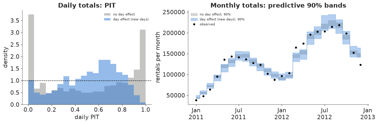
The daily PIT is no longer U-shaped, and daily coverage goes from 65% to 94% (now slightly too wide; the day levels also soak up the Friday and weather-by-hour misfits of section 6). Weekly and monthly coverage improve a lot (36% -> 75%, 25% -> 58%) but stay below 90%: independent day levels still average out over a month, while the calendar showed errors that persist for weeks. The xarray code does not care which model produced the draws - which is the point: once predictions are labelled arrays, checking a new model at every time scale is a re-run, not a rewrite.

8 · The idioms on one page

Task	Named (this notebook)	Instead of
table -> grid	`df.set_index([...]).to_xarray()`	pivot tables and position bookkeeping
per-day attributes	`assign_coords(weekday=("date", ...))`	parallel arrays you must keep in sync
grid -> model rows -> grid	`stack(obs=...)`, `dropna`, `assign_coords(MultiIndex)`, `unstack`	index arithmetic
pick a slice	`.sel(daytype="workday", hour=8)`	`x[:, :, 0, 8]`
thin everything	`idata.isel(draw=slice(None, None, 10))`	thinning each group separately
chains -> samples	`az.extract(idata)`, `.unstack("sample")`	`reshape(-1, ...)`
scenario grid	arithmetic on `DataArray`s with new dims	`np.newaxis` / `reshape` / loops
NumPy function on labelled data	`xr.apply_ufunc(f, *args)`	unpack, call, re-wrap
calendar totals	`.resample(date="W"/"MS").sum()` on draws, then `.quantile`	summing quantiles
rolling / blocks / running total	`.rolling(date=7)`, `.coarsen(date=7)`, `.cumulative("date").sum()`	convolution by hand
binning	`groupby(x=BinGrouper(bins, labels))`, `groupby_bins`	`np.digitize` + masks
cross-tabs	`groupby(hour=BinGrouper(...), weather=UniqueGrouper())`	nested loops
reshape by labels	`set_index(date=[...]).unstack("date")`	building a 3-D array by hand
per-row parameter lookup	`post["a"].sel(daytype=ds.daytype)` (vectorised `.sel`)	`a[:, idx]`
compare models / scenarios	`xr.concat([...], dim=pd.Index([...], name="model"))`	parallel variables

Try it yourself

Correlated days. Holiday weeks and wet spells last several days, but the day levels of section 7 are independent. Give them an AR(1) over date (pm.AR), redo the new-day predictive, and check the weekly and monthly coverage: does it approach 90%?
Riders as a dimension. casual and registered riders behave very differently. Build ds[["casual", "registered"]].to_dataarray("rider"), fit the model with a rider dim on the profile and temperature effects, and facet every figure with col="rider".
A warmer year. Shift every hour's temperature by +2 °C (ds.temp_c + 2), evaluate the posterior mean function on the actual 2012 calendar by broadcasting, and give the change in monthly totals as a fan chart. Which months gain, and which lose?

#1 · From a table to a labelled Dataset

#2 · A modest model with named dimensions

#3 · The DataTree: groups, names and the sample dimension

#Posterior predictive draws, back on the calendar

#4 · Broadcasting by name: counterfactual grids without loops

#A predictive clock: lifting a NumPy RNG with apply_ufunc

#5 · Time machinery on posterior predictive draws

#A fan chart of monthly totals, and a rolling view

#groupby("date.month"), cumulative and .where

#6 · Calibration by bins: where does the model get it wrong?

#The week as a heatmap: the mean, the uncertainty, and the surprise

#A calendar of surprise

#7 · Fixing the day-level misfit, and predicting new days by broadcasting

#8 · The idioms on one page

#Try it yourself