The Luria-Delbrück fluctuation test: jackpots, a likelihood with no closed form, and Bayesian mutation rates

#A Nobel-prize experiment, in one paragraph

In 1943 nobody knew whether bacteria had genes. When a culture of E. coli was exposed to a virus (phage T1), almost every cell died, but a few survivors grew into resistant colonies. Had the virus induced resistance in a few cells it touched, or had resistant mutants arisen at random while the culture grew, before any virus was around? Salvador Luria and Max Delbrück saw that the two stories predict different fluctuations between parallel cultures. If resistance is induced at the moment of exposure, every cell has the same small chance, and the counts of survivors in identical cultures scatter like a Poisson variable (variance = mean). If mutations happen during growth, a mutation that happens early leaves a huge clone of resistant descendants - a jackpot - while most cultures have few or none: the variance is enormous. They found the jackpots. Bacteria mutate spontaneously and selection only picks out what is already there, the result for which Luria and Delbrück shared the 1969 Nobel Prize (with Hershey). The same experiment, the fluctuation test, is still how mutation rates are measured today - for antibiotic resistance, for mutator strains, for cancer cell lines - and its heavy-tailed distribution is still what makes the estimate hard. This notebook fits it in PyMC.

#The plan

1. Two hypotheses, simulated
2. The 1943 data
3. A likelihood with no closed form: the Luria-Delbrück distribution in PyTensor
4. One experiment, five estimators
5. Induced or spontaneous? All ten experiments
6. One mutation rate? A hierarchical model across experiments and media
7. Is the tail heavy enough? Induced + spontaneous, and fitter mutants
8. Why the tail still matters

import logging
import time

import arviz as az
import matplotlib.pyplot as plt
import numpy as np
import pandas as pd
import pymc as pm
import pytensor
import pytensor.tensor as pt
from scipy import linalg, optimize

from pymc_challenges import data

RANDOM_SEED = 53
rng = np.random.default_rng(RANDOM_SEED)
az.style.use("arviz-variat")
logging.getLogger("pymc").setLevel(logging.WARNING)
BLUE, ORANGE, AQUA, GREY, PURPLE, RED, INK = (
    "#2a78d6", "#eb6834", "#1baf7a", "#8a8a86", "#8c5ac8", "#c8384e", "#222222")
print(f"PyMC {pm.__version__}, ArviZ {az.__version__}, PyTensor {pytensor.__version__}")

PyMC 6.3.2, ArviZ 1.3.0, PyTensor 3.3.2

#1 · Two hypotheses, simulated

A culture starts from a small inoculum of $N_0$ sensitive cells and grows exponentially to $N_t$ cells. Measure time in units of $1/\text{growth rate}$, so the culture grows as $N_0 e^{s}$ until $T = \ln(N_t/N_0)$.

• Spontaneous mutation (Darwinian). Each cell division produces a resistant daughter with a small probability $\mu$ (the mutation rate per cell per division). There are $N_t - N_0 \approx N_t$ divisions, so the number of mutations in a culture is Poisson with mean $m = \mu N_t$. Mutations happen in proportion to the number of cells, so most happen late, but a mutation at time $s$ founds a clone that grows for the remaining $T - s$. A clone that starts from one cell and grows by random divisions (a Yule process) has a geometric size at time $T$ with mean $e^{T-s}$. So an early mutation - rare - leaves thousands or millions of resistant cells.
• Induced resistance (Lamarckian). When the phage is added, each of the $N_t$ cells becomes resistant independently with a small probability $a$. The count is Poisson with mean $a N_t$.

We simulate 5,000 cultures of each kind with the scale of Luria and Delbrück's experiment 23 ($N_t = 2.4 \times 10^8$ cells, one mutation per culture on average) and give the induced model the same mean count.

def grow_cultures(mu, n0, nt, n_cultures, rng, fitness=1.0):
    """Resistant cells at the end of growth from n0 to nt cells (spontaneous mutation model).

    Mutations: Poisson(mu * (nt - n0)) per culture, at times with density proportional to the
    population size. A clone founded at time s grows as a Yule process for T - s: its size is
    geometric with success probability exp(-fitness * (T - s)). Clone sizes are capped at nt.
    """
    T = np.log(nt / n0)
    n_mut = rng.poisson(mu * (nt - n0), n_cultures)
    s = np.log1p(rng.uniform(size=n_mut.sum()) * (nt / n0 - 1))     # exponential birth times
    p = np.maximum(np.exp(-fitness * (T - s)), 1.0 / nt)
    clones = rng.geometric(p)
    return np.bincount(np.repeat(np.arange(n_cultures), n_mut), weights=clones,
                       minlength=n_cultures).astype(np.int64)


N_T, N_0, MU_SIM = 2.4e8, 1e3, 1.1 / 2.4e8                          # m = mu * N_t = 1.1
spont = grow_cultures(MU_SIM, N_0, N_T, 5000, rng)
induced = rng.poisson(spont.mean(), 5000)
for name, x in [("spontaneous", spont), ("induced", induced)]:
    print(f"{name:12s} mean {x.mean():6.1f}  variance {x.var():12,.0f}  variance/mean "
          f"{x.var() / x.mean():9,.1f}  zeros {np.mean(x == 0):.2f}  median {np.median(x):4.0f}  "
          f"max {x.max():,}")

fig, axes = plt.subplots(1, 2, figsize=(12, 4))
edges = np.concatenate([[0.5, 1.5, 2.5, 3.5], np.logspace(np.log10(4.5), 8.5, 30)])
for ax, x, c, name in [(axes[0], induced, ORANGE, "induced: Poisson"),
                       (axes[1], spont, BLUE, "spontaneous: Luria-Delbrück")]:
    n_int = np.diff(np.ceil(edges))                   # integers per bin
    h, _ = np.histogram(x + 1, bins=edges)
    ax.stairs(h / len(x) / n_int, edges, fill=True, color=c)
    ax.set(xscale="log", yscale="log", xlim=(0.5, 3e8), ylim=(1e-9, 1),
           xlabel="resistant cells in a culture + 1 (log scale)",
           ylabel="share of cultures per count value", title=f"{name} (mean {x.mean():.0f})")
fig.suptitle("Same mean, different worlds: 5,000 simulated cultures of 2.4e8 cells");

spontaneous  mean    9.7  variance       13,499  variance/mean   1,397.8  zeros 0.33  median    1  max 7,109
induced      mean    9.7  variance           10  variance/mean       1.0  zeros 0.00  median    9  max 21

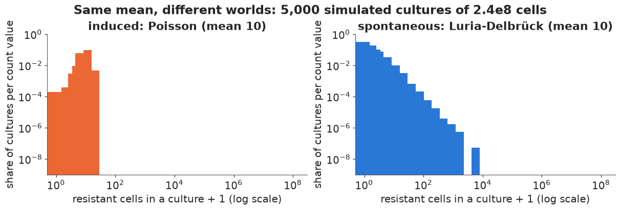
Both sets of cultures have the same average (about 10 resistant cells), but nothing else in common. Induced resistance gives a tight bell around the mean (variance/mean = 1). Spontaneous mutation gives a third of cultures with no resistant cell (no mutation happened: $e^{-1.1}$), a median of 1, and a long tail of jackpots from early mutations reaching thousands of cells - so the variance is more than a thousand times the mean. The sample mean of the spontaneous cultures is itself dominated by a few jackpots, a warning for estimators based on it (section 4).

#2 · The 1943 data

Luria and Delbrück ran three kinds of test. Table 1 is a control: ten samples from one culture, to check that plating itself adds only Poisson noise. Table 2 has eight series of 5-20 parallel cultures; from each culture one sample (a fraction of the culture: 0.05 of 10 ml, or 0.05-0.08 of 0.2 ml) was spread on a plate covered with phage and the resistant colonies counted. Table 3 has two big series (100 and 87 cultures) reported as a frequency table in classes (0, 1, ..., 6-10, 11-20, ..., 501-1000); in experiment 23 the whole culture was plated.

data.describe("luria_delbruck_1943")
ld = data.load("luria_delbruck_1943")
ld["plated"] = ld.sample_ml / ld.culture_ml
print(ld.groupby(["table", "experiment"], sort=False).agg(
    medium=("medium", "first"), cultures=("n_cultures", "sum"), culture_ml=("culture_ml", "first"),
    fraction_plated=("plated", "first"), cells=("cells_per_culture", "first"),
    max_count=("count_hi", "max")).to_string())

luria_delbruck_1943: E. coli B cultures tested for resistance to phage T1 (one row per culture, or per frequency class in table 3). table: 1 = ten samples from ONE culture (plating control), 2 = one sample from each of a series of parallel cultures, 3 = frequency distribution for 100 and 87(88) parallel cultures; experiment; medium (broth or synthetic); culture_ml and sample_ml (the fraction plated is sample_ml / culture_ml); cells_per_culture (bacteria per culture at the time of the test); culture (index); count_lo, count_hi (resistant colonies on the plate: equal for an exact count, a class such as 6-10 in table 3); n_cultures (cultures in that row).
  source: Luria & Delbrueck (1943), Mutations of bacteria from virus sensitivity to virus resistance, Genetics 28:491-511 (PMC1209226), Tables 1-3. TRANSCRIBED from the ESP Foundations reprint at the URL (a PDF, not a CSV) and cross-checked against the dataset `luriadel` of the CRAN package flan (Mazoyer et al.), so keep the cached file in data/. Discrepancies: the reprint omits the 9th culture of experiment 1 (17, in flan; 9 values give the published mean 26.8); experiment 16's 20th culture is 33 in the reprint and 35 in flan (35 gives the published mean 11.35, used here); experiments 10 and 21b average 24.0 and 44.2, not the published 23.8 and 48.2 (both sources agree on the values); experiment 23's frequency classes sum to 88, the paper says 87 cultures.
  url:    http://www.esp.org/foundations/genetics/classical/holdings/l/slmd-43.pdf
                     medium  cultures  culture_ml  fraction_plated         cells  max_count
table experiment                                                                           
1     10a             broth        10         NaN              NaN           NaN         26
      11a             broth        10         NaN              NaN           NaN         65
      3               broth        10         NaN              NaN           NaN          7
2     1               broth         9        10.0            0.005  3.400000e+10        125
      10              broth         8        10.0            0.005  4.000000e+10         41
      11              broth        10        10.0            0.005  4.000000e+10        183
      15              broth        10        10.0            0.005  2.900000e+10        165
      16          synthetic        20         0.2            0.400  5.600000e+08        107
      17          synthetic        12         0.2            0.400  5.000000e+08        303
      21a             broth        19         0.2            0.250  1.100000e+08         19
      21b             broth         5        10.0            0.005  3.200000e+10        107
3     22          synthetic       100         0.2            0.250  2.800000e+08       1000
      23          synthetic        88         0.2            1.000  2.400000e+08       1000

exact = ld[ld.table <= 2]
stats = exact.groupby(["table", "experiment"], sort=False)["count_lo"].agg(["mean", "var", "max"])
stats["var/mean"] = stats["var"] / stats["mean"]
print(stats.round(1).to_string())

tab3 = ld[ld.table == 3]
fig, axes = plt.subplots(1, 2, figsize=(12, 4), width_ratios=[1, 1.4])
ax = axes[0]
for (tab, e), row in stats.iterrows():
    c = GREY if tab == 1 else BLUE
    ax.scatter(row["var/mean"], f"{'T1' if tab == 1 else 'T2'} exp {e}", color=c, s=40, zorder=3)
ax.axvline(1, color=INK, ls=":", lw=1)
ax.set_xscale("log")
ax.set(xlabel="variance / mean of the counts (log)", title="Poisson would give 1")
ax = axes[1]
labels = [f"{lo}" if lo == hi else f"{lo}-{hi}" for lo, hi in
          tab3[tab3.experiment == "22"][["count_lo", "count_hi"]].to_numpy()]
x = np.arange(len(labels))
for k, (e, c) in enumerate([("22", PURPLE), ("23", AQUA)]):
    sub = tab3[tab3.experiment == e]
    ax.bar(x + (k - 0.5) * 0.4, sub.n_cultures / sub.n_cultures.sum(), width=0.4, color=c,
           label=f"exp {e}: {sub.n_cultures.sum()} cultures, plated {sub.plated.iloc[0]:.2f}")
ax.set_xticks(x, labels, rotation=45)
ax.set(xlabel="resistant colonies on the plate (class)", ylabel="share of cultures",
       title="Table 3: most cultures have 0-2, a few have hundreds")
ax.legend(fontsize=8);

                  mean     var  max  var/mean
table experiment                             
1     10a         16.7    18.2   26       1.1
      11a         51.4    38.7   65       0.8
      3            3.3     3.3    7       1.0
2     1           26.8  1400.9  125      52.3
      10          24.0   114.6   41       4.8
      11          62.4  3958.7  183      63.4
      15          26.2  2410.2  165      92.0
      16          11.4   752.1  107      66.3
      17          30.6  7542.3  303     246.6
      21a          3.8    43.8   19      11.6
      21b         44.2  1325.7  107      30.0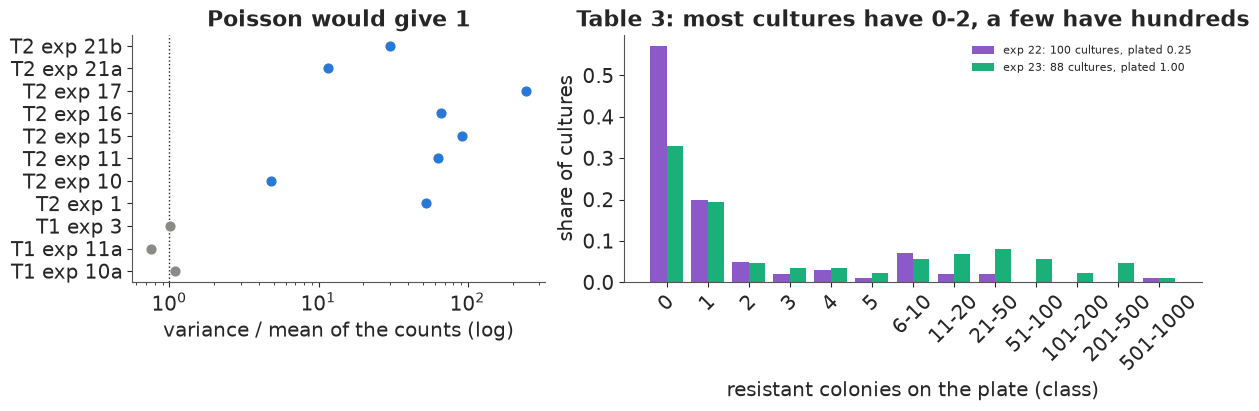

Left: in the plating control (Table 1, grey) the variance is about equal to the mean, as it must be for random samples from one culture. Across parallel cultures (Table 2, blue) the variance/mean ratio is 5 to 250. That is the whole qualitative argument of the paper: the extra variance comes from the cultures, not the plating, and it is far too large for induction. Right: the two big series have the jackpot shape of section 1 - a third to a half of the cultures with no resistant colony and a few with hundreds.

Two notes on the transcription (details in data.describe). In experiment 23 the frequency classes add up to 88 cultures, while the paper says 87 (with 29 zeros); we keep the 88 rows as printed. The widest classes (201-500, 501-1000) hide the exact size of the biggest jackpots - a censoring the likelihood has to respect.

#3 · A likelihood with no closed form

The spontaneous model is a compound Poisson distribution: the number of mutations is Poisson($m$), and each mutation contributes a clone. Section 1 gives the clone size: geometric with mean $1/u$, where $u = e^{-(T-s)}$ is the fraction of the final population that existed when the mutation happened. Because mutations happen in proportion to the population, $u$ is uniform on (0, 1), and averaging the geometric over $u$ gives the clone size distribution

$$P(\text{clone} = k) = \int_0^1 u(1-u)^{k-1}\,du = \frac{1}{k(k+1)}, \qquad k = 1, 2, \dots$$

which has an infinite mean. The number of resistant cells in a culture, the Luria-Delbrück distribution in its Lea-Coulson form, has no closed form, but its probabilities obey a simple recursion (Ma, Sandri & Sarkar 1992). For any compound Poisson with clone-size probabilities $h_j$ and $m$ clones on average,

$$p_0 = e^{-m(1-h_0)}, \qquad p_n = \frac{m}{n}\sum_{j=1}^{n} j\,h_j\,p_{n-j}, \quad n \ge 1,$$

and with $h_j = 1/(j(j+1))$ this is the Ma-Sandri-Sarkar formula $p_n = \frac{m}{n}\sum_{i<n} p_i/(n-i+1)$.

As a linear solve. The recursion says $(I - m A)\,p = p_0 e_0$ with a strictly lower triangular matrix $A_{n,i} = (n-i)\,h_{n-i}/n$. So $p_0,\dots,p_N$ come from one triangular solve, which PyTensor differentiates for us (pt.linalg.solve_triangular): no loop, no scan, exact gradients for NUTS, well under a millisecond for a few hundred terms. The probabilities are all positive and forward substitution only adds positive terms, so it is numerically stable. For very large $m$ the ratio $p_n/p_0$ overflows, so we solve for a rescaled vector.

Extensions in the same frame, each just a different $h_j$:

• Partial plating. If a fraction $\varepsilon$ of the culture is plated, each resistant cell lands on the plate with probability $\varepsilon$: the clone sizes are thinned, which a geometric survives in closed form, so $h_j(\varepsilon)$ is a one-dimensional integral over $u$ (done once, by quadrature, in NumPy). Now $h_0 > 0$: a clone can miss the plate entirely. Luria and Delbrück plated as little as $\varepsilon = 0.005$.
• Induced resistance on top adds Poisson($\lambda$) single cells: $m h_1 \to m h_1 + \lambda$.
• Mutants that grow at a different rate (relative fitness $w$; Mandelbrot 1974, Koch 1982): the clone founded at $u$ is geometric with mean $u^{-w}$; with $\rho = 1/w$ the mixing density becomes $\rho\,u^{\rho-1}$ and $h_j(\rho) = \rho\,B(j, \rho+1)$ (the Yule-Simon distribution). This one depends on a parameter, so the quadrature runs inside the model.

Binned classes enter as $\log \sum_{n \in \text{class}} p_n$. The cost of the solve grows as $N^2$, so we stop the vector at $N = 200$: counts above 200 (only in experiments 22 and 23: the classes 201-500 and 501-1000, six cultures) enter as "more than 200", $\log(1 - \sum_{n \le 200} p_n)$. That throws away a little information about the very largest jackpots and keeps each fit to well under a minute; the predictive checks below use the original classes.

CAP = 200
_t, _w = np.polynomial.legendre.leggauss(400)                  # Gauss-Legendre in log(u)
LOG_U_MIN = -32.0
U = np.exp(0.5 * (_t + 1) * (-LOG_U_MIN) + LOG_U_MIN)
W_U = _w * 0.5 * (-LOG_U_MIN) * U                             # du = u d(log u)


def clone_matrix(eps, N):
    """C[j, q] @ density(u_q) = P(j cells of a clone are plated), j = 0..N.

    A clone with parameter u is geometric on 1, 2, ... with success probability u; thinning each
    cell with probability eps gives P(0) = (1-eps) u/c and P(j) = u/c r^(j-1) ((1-eps) r + eps),
    with c = 1 - (1-u)(1-eps) and r = (1-u) eps / c.
    """
    x = 1 - U
    c = 1 - x * (1 - eps)
    r = x * eps / c
    j = np.arange(1, N + 1)[:, None]
    return np.vstack([(U / c) * (1 - eps), (U / c) * r ** (j - 1) * ((1 - eps) * r + eps)]) * W_U


class Fluctuation:
    """One series of parallel cultures: data, plating fraction, and its likelihood pieces."""

    def __init__(self, rows, cap=CAP):
        rows = rows.loc[rows.index.repeat(rows.n_cultures)]              # one row per culture
        self.name = rows.experiment.iloc[0]
        self.eps = float(rows.plated.iloc[0])
        self.cells = float(rows.cells_per_culture.iloc[0])
        self.synthetic = rows.medium.iloc[0] == "synthetic"
        self.lo = rows.count_lo.to_numpy()
        self.hi = np.where(rows.count_hi > cap, -1, rows.count_hi.to_numpy())   # -1: "> CAP"
        self.N = cap if (self.hi == -1).any() else int(self.lo.max())
        self.C = clone_matrix(self.eps, self.N)
        self.h = self.C.sum(axis=1)                                        # rho = 1 (neutral)
        n = np.arange(self.N + 1)
        lag = n[:, None] - n[None, :]
        self.lag, self.lower = np.where(lag > 0, lag, 0), lag > 0
        self.n_div = np.maximum(n, 1)[:, None]
        self.A = self._a_matrix(self.h)
        self.B = (lag == 1) / self.n_div                                   # induced singles
        self.e0 = (n == 0).astype(float)

    def _a_matrix(self, h, xp=np):
        jh = xp.concatenate([xp.zeros(1), xp.arange(1, self.N + 1) * h[1:]])
        return xp.where(self.lower, jh[self.lag], 0.0) / self.n_div

    def logpmf(self, m, lam=0.0, rho=None):
        """PyTensor: log p_0..p_N (compound Poisson via one triangular solve)."""
        if rho is None:
            h0, A = self.h[0], self.A
        else:
            h = pt.dot(self.C, rho * U ** (rho - 1))
            h0, A = h[0], self._a_matrix(h, xp=pt)
        a = m * (1 - h0) + lam                                   # -log p_0
        shift = pt.maximum(a - 600.0, 0.0)                       # keep p_n / p_0 in range
        x = pt.linalg.solve_triangular(pt.eye(self.N + 1) - m * A - lam * self.B,
                                       pt.exp(shift - a) * self.e0, lower=True)
        return pt.log(x) - shift

    def logpmf_np(self, m, lam=0.0):
        a = m * (1 - self.h[0]) + lam
        shift = max(a - 600.0, 0.0)
        x = linalg.solve_triangular(np.eye(self.N + 1) - m * self.A - lam * self.B,
                                    np.exp(shift - a) * self.e0, lower=True)
        return np.log(x) - shift

    def loglik(self, lp):
        """Per-culture log-likelihood from log p_0..p_N: exact counts, classes, '> CAP'."""
        if (self.lo == self.hi).all():
            return lp[self.lo]
        n = np.arange(self.N + 1)
        cens = self.hi == -1
        lo, hi = np.where(cens, 0, self.lo), np.where(cens, self.N, self.hi)
        mask = np.where((n >= lo[:, None]) & (n <= hi[:, None]), 0.0, -np.inf)
        in_class = pt.logsumexp(lp[None, :] + mask, axis=1)
        return pt.where(cens, pt.log1mexp(pt.minimum(in_class, -1e-300)), in_class)

    def loglik_np(self, lp):
        """NumPy version of loglik, for grids and checks."""
        p = np.exp(lp)
        cdf = np.concatenate([[0.0], np.cumsum(p)])
        cens = self.hi == -1
        hi = np.where(cens, self.N, self.hi)
        mass = np.where(cens, 1 - cdf[-1], cdf[hi + 1] - cdf[np.where(cens, 0, self.lo)])
        return np.log(mass)

    def loglik_poisson(self, lam):
        """Induced model: Poisson counts; a class sums its terms, '> cap' sums 200 terms past it."""
        if (self.lo == self.hi).all():
            return pm.logp(pm.Poisson.dist(lam), self.lo)
        n = np.arange(self.N + 201)
        lp = pm.logp(pm.Poisson.dist(lam), n)
        cens = self.hi == -1
        lo, hi = np.where(cens, self.N + 1, self.lo), np.where(cens, self.N + 200, self.hi)
        mask = np.where((n >= lo[:, None]) & (n <= hi[:, None]), 0.0, -np.inf)
        return pt.logsumexp(lp[None, :] + mask, axis=1)


series = [Fluctuation(ld[ld.experiment == e]) for e in ld[ld.table >= 2].experiment.unique()]
names = [s.name for s in series]
print(pd.DataFrame({"cultures": [len(s.lo) for s in series], "plated": [s.eps for s in series],
                    "N (pmf length - 1)": [s.N for s in series],
                    "P(clone misses plate) h0": [s.h[0].round(3) for s in series]}, index=names))

     cultures  plated  N (pmf length - 1)  P(clone misses plate) h0
1           9   0.005                 125                     0.973
10          8   0.005                  41                     0.973
11         10   0.005                 183                     0.973
15         10   0.005                 165                     0.973
16         20   0.400                 107                     0.389
17         12   0.400                 200                     0.389
21a        19   0.250                  19                     0.538
21b         5   0.005                 107                     0.973
22        100   0.250                 200                     0.538
23         88   1.000                 200                     0.000

Now the checks, before any fitting (the rule from E32: a new likelihood gets unit tests). The triangular solve should reproduce the textbook recursion; and the distribution should match simulated cultures - the physical simulation of section 1 for full plating, and cultures sampled at $\varepsilon = 0.005$ like the 10 ml experiments.

def mss_recursion(m, N):
    p = np.zeros(N + 1)
    p[0] = np.exp(-m)
    for n in range(1, N + 1):
        p[n] = m / n * np.sum(p[:n] / (n - np.arange(n) + 1))
    return p


full = Fluctuation(pd.DataFrame({"experiment": ["check"], "plated": [1.0], "cells_per_culture": [N_T],
                                 "medium": ["-"], "count_lo": [300], "count_hi": [300],
                                 "n_cultures": [1]}), cap=300)
m_chk = 1.1
p_solve = np.exp(full.logpmf_np(m_chk))
print(f"max |solve - MSS recursion| = {np.abs(p_solve - mss_recursion(m_chk, 300)).max():.1e}")
m_sym = pt.dscalar("m")
f_pt = pytensor.function([m_sym], full.logpmf(m_sym))
print(f"max |PyTensor - NumPy| (log p) = {np.abs(f_pt(m_chk) - full.logpmf_np(m_chk)).max():.1e}")

# partial plating: 20,000 simulated 10 ml cultures, 0.05 ml plated, m = 600 mutations per culture
tenml = Fluctuation(ld[ld.experiment == "1"].assign(count_lo=300, count_hi=300), cap=300)
m_10 = 600.0
cult = grow_cultures(m_10 / 3.4e10, 1e3, 3.4e10, 20000, rng)
plated = rng.binomial(cult, tenml.eps)
p_thin = np.exp(tenml.logpmf_np(m_10))

fig, axes = plt.subplots(1, 2, figsize=(12, 4))
def tv_distance(sample, p):
    """Total variation between a sample's histogram on 0..len(p)-1 (+ one tail cell) and p."""
    emp = np.bincount(np.minimum(sample, len(p)), minlength=len(p) + 1) / len(sample)
    return 0.5 * np.abs(emp - np.append(p, 1 - p.sum())).sum(), emp[:len(p)]


for ax, sim, p, eps, m_, title in [
        (axes[0], spont, p_solve, 1.0, m_chk, "whole culture plated, m = 1.1"),
        (axes[1], plated, p_thin, tenml.eps, m_10, "0.5% of a 10 ml culture plated, m = 600")]:
    n = np.arange(len(p))
    tv, emp = tv_distance(sim, p)
    p_ext = np.append(p, 1 - p.sum())
    tv_ref = np.mean([tv_distance(rng.choice(len(p_ext), len(sim), p=p_ext), p)[0]
                      for _ in range(20)])                      # same-size samples from the pmf itself
    ax.loglog(n[1:], emp[1:], "o", color=GREY, ms=3, label=f"simulated cultures ({len(sim):,})")
    ax.loglog(n[1:], p[1:], color=BLUE, lw=2, label="Luria-Delbrück pmf (triangular solve)")
    ax.loglog(n[10:], m_ * eps / n[10:] ** 2, color=ORANGE, ls="--", lw=1,
              label="m eps / n^2 (one big clone)")
    ax.set(xlabel="resistant colonies n", ylabel="P(n)", title=title)
    print(f"{title}: P(0) simulated {emp[0]:.3f}, model {p[0]:.3f}; P(n <= 300) simulated "
          f"{np.mean(sim <= 300):.4f}, model {p.sum():.4f}; TV distance {tv:.3f} "
          f"(pure sampling noise at this size: {tv_ref:.3f})")
    ax.legend(fontsize=8)
del cult, plated

max |solve - MSS recursion| = 1.4e-13

max |PyTensor - NumPy| (log p) = 0.0e+00

whole culture plated, m = 1.1: P(0) simulated 0.335, model 0.333; P(n <= 300) simulated 0.9966, model 0.9963; TV distance 0.042 (pure sampling noise at this size: 0.037)
0.5% of a 10 ml culture plated, m = 600: P(0) simulated 0.000, model 0.000; P(n <= 300) simulated 0.9879, model 0.9888; TV distance 0.025 (pure sampling noise at this size: 0.028)

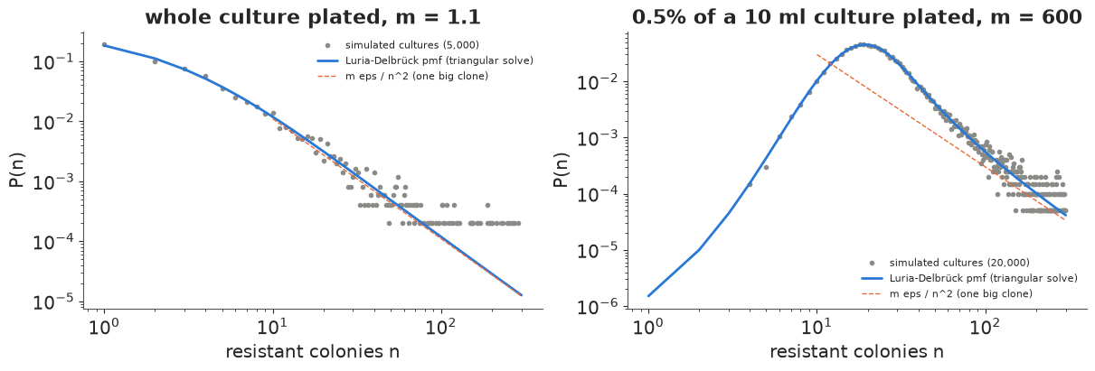
The solve agrees with the recursion to rounding error, and the PyTensor graph with the NumPy one. The distribution matches the simulated cultures in both regimes, including the zeros and the probability mass beyond 300. The total-variation distances are what sampling noise alone gives for samples of this size (printed next to them). (The physical simulation starts from $N_0 = 1000$ cells, not from zero as the Lea-Coulson limit assumes; the difference is invisible at this scale.) The tail approaches $m\varepsilon/n^2$ (dashed), the chance that a single early clone put $n$ cells on the plate: that is the jackpot, and it is why the mean number of mutants is useless (infinite in the limit) while the probabilities are perfectly well behaved. Thinning ($\varepsilon = 0.005$) does not change the tail exponent, only where it starts: with 600 clones per culture the plate count has a body around 20 and bends into the $n^{-2}$ tail only beyond about 200.

#4 · One experiment, five estimators

Experiment 23 plated whole cultures, which makes every classic estimator applicable. With $C$ cultures:

• Mean method (Luria & Delbrück's equation 8): the average count $\bar r$ satisfies $\bar r = m \ln(C m)$; solve for $m$. It uses the mean, which the jackpots dominate.
• $p_0$ method (their equation 5): the share of cultures with no mutant is $e^{-m}$, so $m = -\ln p_0$. It throws away every non-zero count and fails when $m > 4$ or so (no zeros).
• Lea-Coulson median: $\tilde r/m - \ln m = 1.24$. Designed for $m$ of about 4 or more.
• Maximum likelihood with the distribution of section 3 (the modern standard, e.g. in the rSalvador and flan R packages).
• Bayesian posterior of the same likelihood, which gives an interval that respects the skewness of the likelihood.

Luria and Delbrück report $\bar r = 28.6$ resistant bacteria per culture in experiment 23 (the classes alone do not give the mean). We report $\mu = m/N_t$, mutations per cell per division - numerically the same as their "mutation rate per bacterium per time unit" (they also quote a per-division-cycle value, smaller by a factor $\ln 2$, from a different time convention).

e23 = series[names.index("23")]
C23, R_BAR23 = len(e23.lo), 28.6
n_zero = int(np.sum(e23.hi == 0))
m_mean = optimize.brentq(lambda m: m * np.log(C23 * m) - R_BAR23, 0.05, 100)
m_p0 = -np.log(n_zero / C23)
median23 = np.median(e23.lo)
m_median = optimize.brentq(lambda m: median23 / m - np.log(m) - 1.24, 0.01, 50)
assert np.allclose(e23.loglik_np(e23.logpmf_np(1.1)),                 # NumPy == PyTensor
                   pytensor.function([], e23.loglik(pt.as_tensor(e23.logpmf_np(1.1))))())
m_mle = float(np.exp(optimize.minimize_scalar(
    lambda lm: -e23.loglik_np(e23.logpmf_np(np.exp(lm))).sum(),
    bounds=(np.log(0.2), np.log(10)), method="bounded").x))

with pm.Model() as m23:
    log10_mu = pm.Normal("log10_mu", -8.0, 1.0)
    m = pm.Deterministic("m", 10 ** log10_mu * e23.cells)
    pm.Potential("lik", e23.loglik(e23.logpmf(m)).sum())
    idata23 = pm.sample(random_seed=RANDOM_SEED, progressbar=False)
print(az.summary(idata23, var_names=["log10_mu", "m"], round_to=3))
print("divergences:", int(idata23.sample_stats["diverging"].sum()),
      "| tuning steps:", idata23.posterior.attrs.get("tuning_steps"))

m_post = idata23.posterior["m"].to_numpy().ravel()
est = pd.DataFrame({
    "m": [m_mean, m_p0, m_median, m_mle, np.median(m_post)],
    "89% interval": ["", "", "", "", f"{np.quantile(m_post, 0.055):.2f}-{np.quantile(m_post, 0.945):.2f}"]},
    index=["mean (LD eq. 8)", f"p0 ({n_zero}/{C23} zeros)", f"Lea-Coulson median (median {median23:.0f})",
           "maximum likelihood", "posterior median"])
est["mu = m / N_t (x 1e-8)"] = (est["m"] / e23.cells * 1e8).round(2)
print(est.round(2).to_string())

           mean     sd  eti89_lb  eti89_ub  ess_bulk  ess_tail  r_hat  \
log10_mu -8.295  0.054    -8.383    -8.214  1467.836  2004.776  1.002   
m         1.226  0.152     0.994     1.467  1467.836  2004.776  1.002   

          mcse_mean  mcse_sd  
log10_mu      0.001    0.001  
m             0.004    0.002  
divergences: 0 | tuning steps: 400
                                  m 89% interval  mu = m / N_t (x 1e-8)
mean (LD eq. 8)                4.74                                1.98
p0 (29/88 zeros)               1.11                                0.46
Lea-Coulson median (median 1)  0.89                                0.37
maximum likelihood             1.22                                0.51
posterior median               1.22    0.99-1.47                   0.51

The estimators disagree by a factor of four. The mean method gives $\mu \approx 2 \times 10^{-8}$ (Luria and Delbrück's Table 4 lists $2.4 \times 10^{-8}$ for this experiment; we cannot reproduce their number from the printed mean with equation 8, but the order is the same). The $p_0$ method, the MLE and the posterior agree on 1.1-1.2 mutations per culture, $\mu \approx 0.5 \times 10^{-8}$ (Luria and Delbrück's own $p_0$ value was $0.47 \times 10^{-8}$), with the posterior giving an 89% interval of about 1.0-1.5. The median method is lower (0.9); with a median of 1 it is far outside the range the formula was made for. Luria and Delbrück noticed that their mean-method rates were "all higher" than the $p_0$ rate and blamed an excess of early mutations: the jackpots. Which estimator is right in general? A simulation study answers that better than one data set: draw many experiments from the model with a known $m$ and estimate $m$ each time.

def simulate_experiment(m, n_cultures, rng):
    """Whole-culture counts from the Lea-Coulson model: Poisson(m) clones of size 1/(k(k+1))."""
    k = rng.poisson(m, n_cultures)
    u = rng.uniform(size=k.sum())
    clones = rng.geometric(np.maximum(u, 1e-12))
    return np.bincount(np.repeat(np.arange(n_cultures), k), weights=clones,
                       minlength=n_cultures).astype(np.int64)


CAP_SIM = 2000
grid_sim = np.exp(np.linspace(np.log(0.1), np.log(100), 160))
big = Fluctuation(pd.DataFrame({"experiment": ["sim"], "plated": [1.0], "cells_per_culture": [N_T],
                                "medium": ["-"], "count_lo": [CAP_SIM], "count_hi": [CAP_SIM],
                                "n_cultures": [1]}), cap=CAP_SIM)
LOGP = np.array([big.logpmf_np(m) for m in grid_sim])                   # (grid, 0..CAP_SIM)
LOGP_TAIL = np.log1p(-np.minimum(np.exp(LOGP).sum(axis=1), 1 - 1e-15))   # "more than CAP_SIM"
del big


def estimators(r):
    C = len(r)
    out = {"mean": optimize.brentq(lambda m: m * np.log(C * m) - r.mean(), 1e-3, 1e5)}
    z = np.mean(r == 0)
    out["p0"] = -np.log(z) if z > 0 else np.nan
    med = np.median(r)
    out["median"] = (optimize.brentq(lambda m: med / m - np.log(m) - 1.24, 1e-3, 1e4)
                     if med > 0 else np.nan)
    counts = np.bincount(np.minimum(r, CAP_SIM + 1), minlength=CAP_SIM + 2)
    ll = LOGP @ counts[:CAP_SIM + 1] + LOGP_TAIL * counts[CAP_SIM + 1]
    out["MLE"] = grid_sim[np.argmax(ll)]
    return out


designs = [(1.1, 87), (20.0, 30)]
study = {}
for m_true, C in designs:
    rows = [estimators(simulate_experiment(m_true, C, rng)) for _ in range(400)]
    study[(m_true, C)] = pd.DataFrame(rows)
    summary = {}
    for k, v in study[(m_true, C)].items():
        r = np.log2(v.dropna() / m_true)
        summary[k] = ({"median ratio": 2 ** r.median(), "log2 5%": r.quantile(0.05),
                       "log2 95%": r.quantile(0.95)} if len(r) else {}) | {"undefined": v.isna().mean()}
    print(f"true m = {m_true}, {C} cultures, 400 simulated experiments")
    print(pd.DataFrame(summary).T.round(2).to_string())

fig, axes = plt.subplots(1, 2, figsize=(12, 4), sharey=True)
for ax, (m_true, C) in zip(axes, designs):
    s = study[(m_true, C)]
    for i, (k, c) in enumerate(zip(s.columns, [ORANGE, PURPLE, GREY, BLUE])):
        v = np.log2(s[k].dropna() / m_true)
        if len(v) == 0:
            continue
        ax.scatter(v, i + rng.uniform(-0.25, 0.25, len(v)), s=4, color=c, alpha=0.4)
        ax.plot(np.quantile(v, [0.05, 0.95]), [i, i], color=INK, lw=2)
        ax.plot(np.median(v), i, "o", color=INK, ms=5)
    ax.axvline(0, color=INK, ls=":", lw=1)
    ax.set_yticks(range(4), ["mean (1943)", "p0", "Lea-Coulson median", "MLE"])
    ax.set(xlabel="log2(estimate / true m)", title=f"m = {m_true}, {C} cultures")
axes[1].text(0.02, 0.4, "p0 undefined: no culture\nwithout mutants, ever", transform=axes[1].transAxes,
             fontsize=8, color=PURPLE);

true m = 1.1, 87 cultures, 400 simulated experiments
        median ratio  log2 5%  log2 95%  undefined
mean            1.27    -0.41      2.52        0.0
p0              1.00    -0.27      0.32        0.0
median          0.81    -0.31      0.26        0.0
MLE             0.99    -0.26      0.24        0.0
true m = 20.0, 30 cultures, 400 simulated experiments
        median ratio  log2 5%  log2 95%  undefined
mean            1.20    -0.30      1.71        0.0
p0               NaN      NaN       NaN        1.0
median          1.01    -0.25      0.32        0.0
MLE             1.00    -0.25      0.19        0.0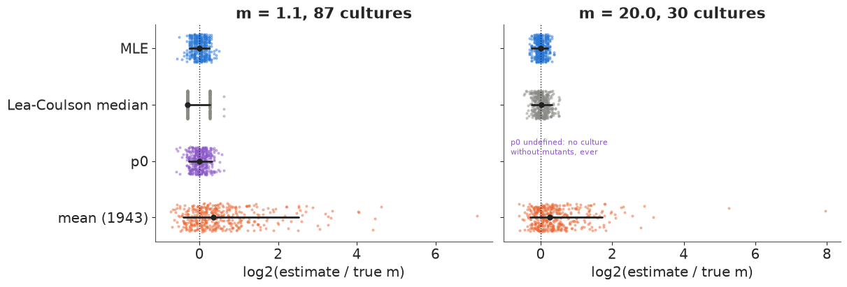

The simulation study (400 simulated experiments per design) makes the ranking general. The mean method is biased upwards (median 20% high) and has by far the widest scatter, up to fourfold too high in 5% of experiments: whether an experiment happened to contain one giant jackpot decides the answer. $p_0$ is unbiased at $m = 1.1$ (within about 25% in 90% of experiments) but, with $m = 20$, no culture is ever free of mutants and it does not exist. The median method is biased about 20% low at $m = 1.1$ - with a median of 0, 1 or 2 it can take only a few values - and fine at $m = 20$, where it was designed to work. Maximum likelihood is centred on the truth in both designs with the narrowest spread (within about 20-25% in 90% of experiments). The posterior uses the same likelihood, so it inherits these properties and adds an honest interval. That is why the field moved to likelihood-based estimation in the 1990s-2000s (Ma, Sandri & Sarkar; Rosche & Foster 2000; Zheng's rSalvador) and why a heavy-tailed likelihood that a sampler can use matters.

#5 · Induced or spontaneous? All ten experiments

Now the question of 1943, with all 281 cultures. Each experiment gets its own rate, tied together by a hierarchical prior (section 6 looks at that part):

$$\log_{10}\text{rate}_e = \beta_0 + \beta_\text{syn}\,[\text{synthetic medium}]_e + \tau z_e, \qquad z_e \sim N(0, 1).$$

• Induced: plated colonies are Poisson with mean $a_e N_e \varepsilon_e$.
• Spontaneous: the Luria-Delbrück distribution with $m_e = \mu_e N_e$, thinned by the plated fraction $\varepsilon_e$.

Priors: $\beta_0 \sim N(-8, 1)$ (a rate between $10^{-10}$ and $10^{-6}$ per cell is plausible for a single-gene phenotype; in experiment 23 that is 0.02-200 mutations per culture), $\beta_\text{syn} \sim N(0, 0.5)$ (no medium effect expected, a threefold one allowed), $\tau \sim \text{HalfNormal}(0.3)$ (experiments agree to within a factor of about 2). The likelihood is a pm.Potential, so we store each culture's log-likelihood as a Deterministic and hand it to ArviZ for PSIS-LOO ourselves.

SYN = np.array([s.synthetic for s in series], dtype=float)
coords = {"experiment": names, "culture": np.arange(sum(len(s.lo) for s in series))}


def fluctuation_model(kind="spontaneous", induced_extra=False, fitness=False):
    with pm.Model(coords=coords) as model:
        b0 = pm.Normal("b0", -8.0, 1.0)
        b_syn = pm.Normal("b_syn", 0.0, 0.5)
        tau = pm.HalfNormal("tau", 0.3)
        z = pm.Normal("z", 0.0, 1.0, dims="experiment")
        log10_rate = pm.Deterministic("log10_rate", b0 + b_syn * SYN + tau * z, dims="experiment")
        if induced_extra:                                  # one induced rate shared by all
            log10_a = pm.Normal("log10_a", -8.0, 1.0)
        rho = pm.LogNormal("rho", 0.0, 0.5) if fitness else None
        lls = []
        for k, s in enumerate(series):
            if kind == "induced":
                lls.append(s.loglik_poisson(10 ** log10_rate[k] * s.cells * s.eps))
                continue
            lam = 10 ** log10_a * s.cells * s.eps if induced_extra else 0.0
            lls.append(s.loglik(s.logpmf(10 ** log10_rate[k] * s.cells, lam, rho)))
        ll = pm.Deterministic("ll", pt.concatenate(lls), dims="culture")
        pm.Potential("likelihood", ll.sum())
    return model


def fit(model, **kw):
    t0 = time.time()
    idata = pm.sample(random_seed=RANDOM_SEED, progressbar=False, model=model, **kw)
    idata["log_likelihood"] = idata.posterior["ll"].to_dataset(name="y")
    idata["posterior"] = idata.posterior.to_dataset().drop_vars("ll")
    loo = az.loo(idata, var_name="y", pointwise=True)
    loo.log_weights = None
    del idata["log_likelihood"]
    st = idata.sample_stats
    print(f"{time.time() - t0:.0f} s | divergences {int(st['diverging'].sum())} | "
          f"max r_hat {float(az.rhat(idata).to_dataset().to_dataarray().max()):.3f} | "
          f"min ess_bulk {float(az.ess(idata).to_dataset().to_dataarray().min()):.0f} | "
          f"elpd_loo {loo.elpd:.1f} | Pareto k > 0.7: {int((loo.pareto_k > 0.7).sum())}")
    return idata, loo


fits, loos = {}, {}
fits["induced"], loos["induced"] = fit(fluctuation_model("induced"))
fits["spontaneous"], loos["spontaneous"] = fit(fluctuation_model("spontaneous"), target_accept=0.9)
print(az.compare({k: loos[k] for k in ["induced", "spontaneous"]}, round_to=1)[
    ["rank", "elpd", "elpd_diff", "dse", "p"]])

23 s | divergences 0 | max r_hat 1.007 | min ess_bulk 517 | elpd_loo -5700.6 | Pareto k > 0.7: 18

15 s | divergences 0 | max r_hat 1.006 | min ess_bulk 780 | elpd_loo -671.2 | Pareto k > 0.7: 0
             rank    elpd  elpd_diff    dse      p
spontaneous     0  -671.2        0.0    0.0   12.8
induced         1 -5700.6    -5029.5  960.4  481.1

Both samplers ran cleanly (no divergences, r_hat at most 1.01). The comparison is not close: the spontaneous model's expected log predictive density is higher by about 5,000 units, five times its (large) standard error. The induced model also has 18 cultures with Pareto $k > 0.7$ - single jackpot cultures that the Poisson fit cannot predict without having seen them; its LOO estimate is unreliable, but only in the direction of being even worse. A predictive check shows the same thing in a picture: for each experiment, the largest count among its cultures, observed vs. replicated from each posterior.

def replicate_counts(s, m, lam, rho, rng):
    """Posterior predictive counts for one series: thinned clones + induced singles."""
    k = rng.poisson(m)
    u = rng.uniform(size=k.sum())
    p = np.maximum(u ** (1.0 / rho), 1.0 / s.cells)            # geometric parameter, fitness 1/rho
    plated = rng.binomial(rng.geometric(p), s.eps)
    idx = np.repeat(np.arange(len(m)), k)
    return np.bincount(idx, weights=plated, minlength=len(m)).astype(np.int64) + rng.poisson(lam, len(m))


def ppc_max(idata, kind, n_draws=300, lam_var=None, rho_var=None):
    extra = az.extract(idata, num_samples=n_draws, random_seed=RANDOM_SEED)
    post = extra["log10_rate"].transpose("experiment", "sample").to_numpy()
    out = np.zeros((len(series), n_draws))
    stat_rng = np.random.default_rng(RANDOM_SEED)
    for k, s in enumerate(series):
        for d in range(n_draws):
            if kind == "induced":
                r = stat_rng.poisson(10 ** post[k, d] * s.cells * s.eps, len(s.lo))
            else:
                lam = 10 ** float(extra[lam_var][d]) * s.cells * s.eps if lam_var else 0.0
                rho = float(extra[rho_var][d]) if rho_var else 1.0
                r = replicate_counts(s, np.full(len(s.lo), 10 ** post[k, d] * s.cells), lam, rho,
                                     stat_rng)
            out[k, d] = r.max()
    return out


obs_max = np.array([s.lo.max() for s in series])        # 501 in exps 22, 23 means "at least 501"
ppc = {k: ppc_max(fits[k], k) for k in ["induced", "spontaneous"]}
for k, rep in ppc.items():
    lo, hi = np.quantile(rep, [0.05, 0.95], axis=1)
    print(f"{k:12s}: observed maximum inside the 90% predictive interval in "
          f"{np.sum((obs_max >= lo) & (obs_max <= hi))} of {len(series)} series; above it in "
          f"{np.sum(obs_max > hi)} ({', '.join(np.array(names)[obs_max > hi])})")


def plot_ppc_max(ax, ppcs, colours):
    for j, ((label, rep), c) in enumerate(zip(ppcs.items(), colours)):
        y = np.arange(len(series)) + (j - (len(ppcs) - 1) / 2) * 0.22
        lo, mid, hi = np.quantile(rep + 1, [0.05, 0.5, 0.95], axis=1)
        ax.hlines(y, lo, hi, color=c, lw=3, alpha=0.8, label=f"{label} (90% predictive)")
        ax.plot(mid, y, "|", color=c, ms=8)
    ax.plot(obs_max + 1, np.arange(len(series)), "D", color=INK, ms=6, label="observed")
    ax.set_xscale("log")
    ax.set_yticks(range(len(series)), [f"exp {n} ({'syn' if s.synthetic else 'broth'})"
                                       for n, s in zip(names, series)])
    ax.set(xlabel="largest count among the cultures + 1 (log)")
    ax.legend(fontsize=8, loc="lower right")


fig, ax = plt.subplots(figsize=(10, 5))
plot_ppc_max(ax, ppc, [ORANGE, BLUE])
ax.set_title("Posterior predictive check of the jackpots: the largest culture in each series");

induced     : observed maximum inside the 90% predictive interval in 0 of 10 series; above it in 10 (1, 10, 11, 15, 16, 17, 21a, 21b, 22, 23)
spontaneous : observed maximum inside the 90% predictive interval in 9 of 10 series; above it in 1 (17)

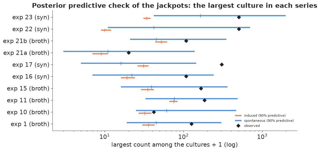
Under induction (orange) the largest culture of every series should be within a factor of about two of the typical count. The observed maxima (black diamonds; for experiments 22 and 23 the lower edge of the "more than 500" class) are above those intervals in all ten series. Under spontaneous mutation (blue) the predictive intervals of the maximum span one to two orders of magnitude - that is what jackpots look like - and nine of the ten observed maxima fall inside them. The exception is experiment 17, whose one culture with 303 colonies is above the interval. The spontaneous model is right about the kind of variation. Whether it gets the size of the tail right is section 7.

#6 · One mutation rate? A hierarchical model across experiments and media

Luria and Delbrück concluded from their Table 4 (mean method) that the mutation rate "does not vary greatly from experiment to experiment" and does not differ between broth and synthetic medium, despite very different growth rates. The hierarchical model asks the same question with the full likelihood.

LD_TABLE4 = {"1": 1.8, "10": 1.4, "11": 4.1, "15": 2.1, "16": 1.1, "17": 3.0, "21a": 3.3,
             "21b": 3.0, "22": 2.3, "23": 2.4}                   # x 1e-8, mean method (Table 4)
print(az.summary(fits["spontaneous"], var_names=["b0", "b_syn", "tau"], round_to=3))
bs = fits["spontaneous"].posterior["b_syn"].to_numpy().ravel()
print(f"synthetic / broth mutation rate: {np.median(10 ** bs):.2f} "
      f"(89% interval {np.quantile(10 ** bs, 0.055):.2f}-{np.quantile(10 ** bs, 0.945):.2f}); "
      f"P(lower in synthetic) = {np.mean(bs < 0):.3f}")


def log_ticks(ax, ticks=(0.2, 0.5, 1, 2, 5)):
    ax.set_xscale("log")
    ax.set_xticks(ticks, [f"{t:g}" for t in ticks])
    ax.xaxis.set_minor_formatter(plt.NullFormatter())


def plot_rates(ax, idata, colour, label, offset):
    r = 10 ** (idata.posterior["log10_rate"].to_numpy().reshape(-1, len(series)) + 8)
    lo, mid, hi = np.quantile(r, [0.055, 0.5, 0.945], axis=0)
    y = np.arange(len(series)) + offset
    ax.hlines(y, lo, hi, color=colour, lw=3, alpha=0.8, label=label)
    ax.plot(mid, y, "o", color=colour, ms=5)


fig, ax = plt.subplots(figsize=(10, 5))
plot_rates(ax, fits["spontaneous"], BLUE, "posterior, Luria-Delbrück likelihood (89%)", 0.0)
ax.plot([LD_TABLE4[n] for n in names], np.arange(len(series)) - 0.25, "s", color=ORANGE,
        label="Luria & Delbrück 1943, mean method (Table 4)")
log_ticks(ax)
ax.set_yticks(range(len(series)), [f"exp {n} ({'syn' if s.synthetic else 'broth'}, "
                                   f"{s.eps:.3g} plated)" for n, s in zip(names, series)])
ax.set(xlabel="mutation rate mu (x 1e-8 per cell per division, log)",
       title="Per-experiment mutation rates")
ax.legend(fontsize=8);
post_med = np.median(10 ** (fits["spontaneous"].posterior["log10_rate"].to_numpy().reshape(-1, len(series)) + 8),
                     axis=0)
print(pd.DataFrame({"posterior median": post_med.round(2), "LD Table 4": [LD_TABLE4[n] for n in names],
                    "Table 4 / posterior": (np.array([LD_TABLE4[n] for n in names]) / post_med).round(1)},
                   index=names).T.to_string())

        mean     sd  eti89_lb  eti89_ub  ess_bulk  ess_tail  r_hat  mcse_mean  \
b0    -7.899  0.065    -8.001    -7.799   995.897  1165.614  1.006      0.002   
b_syn -0.505  0.102    -0.664    -0.347  1221.523  1565.647  1.006      0.003   
tau    0.124  0.058     0.042     0.220   779.875   956.344  1.002      0.002   

       mcse_sd  
b0       0.002  
b_syn    0.003  
tau      0.002  
synthetic / broth mutation rate: 0.31 (89% interval 0.22-0.45); P(lower in synthetic) = 1.000
                        1    10    11    15   16    17   21a   21b    22    23
posterior median     1.13  1.32  1.48  1.05  0.3  0.37  1.19  1.71  0.43  0.48
LD Table 4           1.80  1.40  4.10  2.10  1.1  3.00  3.30  3.00  2.30  2.40
Table 4 / posterior  1.60  1.10  2.80  2.00  3.6  8.10  2.80  1.80  5.40  5.00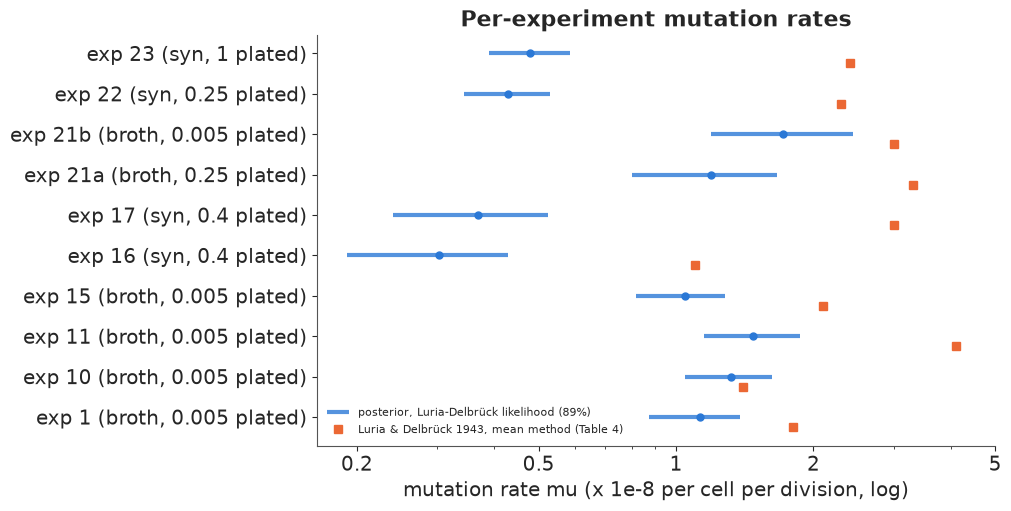

Two things change with the likelihood. First, every rate is lower than the mean-method value, by a factor of 1.1 (experiment 10) to 8 (experiment 17) - the jackpot bias of section 4, now in every experiment. Second, the experiments separate into two groups: the synthetic-medium series (16, 17, 22, 23) come out about three times lower than the broth series (ratio 0.31, 89% interval 0.22-0.45), and every posterior draw has "lower in synthetic". The mean method's noise had hidden this; Luria and Delbrück's conclusion of "no difference" does not survive the full likelihood - at least not with this model. Before believing it we have to ask whether the model is adequate: the broth series are mostly the 10 ml cultures with only 0.5% plated, whose counts are made almost entirely of large clones, so their rates depend on the shape of the tail more than any other series. The remaining between-experiment spread is small ($\tau \approx 0.12$ in $\log_{10}$, about 30%).

#7 · Is the tail heavy enough?

Holmes, Ghafari, Abbas, Saravanan & Nemenman (2017, arXiv:1701.05627) re-analysed experiments 22 and 23 and found that experiment 23 has a tail heavier than the Luria-Delbrück model predicts, and that a model with both induced and spontaneous resistance could not be ruled out on experiment 22. We test two extensions on all ten series:

1. Induced + spontaneous: one extra Poisson($a N \varepsilon$) of induced survivors, with the induced probability $a$ shared by all experiments (it is a property of the cell-phage encounter). This makes the body of the distribution more Poisson-like; it cannot fatten the tail.
2. Differential growth (Mandelbrot-Koch): mutants grow at relative rate $w = 1/\rho$; $\rho < 1$ (faster mutants) fattens the tail, $\rho > 1$ thins it. Prior $\rho \sim \text{LogNormal}(0, 0.5)$.

We look at experiment 23's frequency table under each model after fitting them.

fits["induced + spontaneous"], loos["induced + spontaneous"] = fit(
    fluctuation_model("spontaneous", induced_extra=True), target_accept=0.9)
fits["fitness"], loos["fitness"] = fit(fluctuation_model("spontaneous", fitness=True),
                                       target_accept=0.9)
print(az.compare(loos, round_to=1)[["rank", "elpd", "elpd_diff", "dse", "p", "weight"]])
print(az.summary(fits["fitness"], var_names=["rho", "b0", "b_syn", "tau"], round_to=3))
print(az.summary(fits["induced + spontaneous"], var_names=["log10_a"], round_to=3))

21 s | divergences 0 | max r_hat 1.004 | min ess_bulk 867 | elpd_loo -672.0 | Pareto k > 0.7: 1

38 s | divergences 0 | max r_hat 1.003 | min ess_bulk 778 | elpd_loo -649.2 | Pareto k > 0.7: 0
                       rank    elpd  elpd_diff    dse      p  weight
fitness                   0  -649.2        0.0    0.0    8.2     1.0
spontaneous               1  -671.2      -21.9    6.8   12.8     0.0
induced + spontaneous     2  -672.0      -22.7    6.9   12.8     0.0
induced                   3 -5700.6    -5051.4  964.6  481.1     0.0
        mean     sd  eti89_lb  eti89_ub  ess_bulk  ess_tail  r_hat  mcse_mean  \
rho    0.711  0.042     0.642     0.778  1756.089  1889.831  1.000      0.001   
b0    -8.326  0.103    -8.494    -8.169  1217.472  1417.030  1.001      0.003   
b_syn -0.148  0.122    -0.349     0.043  1200.586  1078.378  1.003      0.004   
tau    0.125  0.067     0.033     0.238   777.962   914.233  1.003      0.002   

       mcse_sd  
rho      0.001  
b0       0.002  
b_syn    0.003  
tau      0.003  
          mean     sd  eti89_lb  eti89_ub  ess_bulk  ess_tail  r_hat  \
log10_a -9.953  0.466   -10.774    -9.324  4138.603  2225.992  1.001   

         mcse_mean  mcse_sd  
log10_a      0.008     0.01  

a_post = fits["induced + spontaneous"].posterior["log10_a"].to_numpy().ravel()
mu23 = 10 ** fits["induced + spontaneous"].posterior["log10_rate"].sel(experiment="23").to_numpy().ravel()
lam23 = 10 ** a_post * e23.cells
print(f"induced resistance probability a: 95% upper bound {10 ** np.quantile(a_post, 0.95):.1e} per cell"
      f" | experiment 23: induced survivors per culture (95% upper) {np.quantile(lam23, 0.95):.2f}"
      f" vs mutations per culture {np.median(mu23 * e23.cells):.2f}")
rho_post = fits["fitness"].posterior["rho"].to_numpy().ravel()
print(f"relative growth rate of mutants w = 1/rho: {np.median(1 / rho_post):.2f} "
      f"(89% interval {np.quantile(1 / rho_post, 0.055):.2f}-{np.quantile(1 / rho_post, 0.945):.2f})")
bs_f = fits["fitness"].posterior["b_syn"].to_numpy().ravel()
print(f"fitness model: synthetic / broth rate {np.median(10 ** bs_f):.2f} "
      f"(89% {np.quantile(10 ** bs_f, 0.055):.2f}-{np.quantile(10 ** bs_f, 0.945):.2f}); "
      f"P(lower in synthetic) = {np.mean(bs_f < 0):.3f}")

induced resistance probability a: 95% upper bound 4.9e-10 per cell | experiment 23: induced survivors per culture (95% upper) 0.12 vs mutations per culture 1.13
relative growth rate of mutants w = 1/rho: 1.41 (89% interval 1.29-1.56)
fitness model: synthetic / broth rate 0.72 (89% 0.45-1.10); P(lower in synthetic) = 0.893

classes = tab3[tab3.experiment == "23"][["count_lo", "count_hi", "n_cultures"]].to_numpy()
cls_hi = np.where(classes[:, 1] == 1000, np.inf, classes[:, 1])       # top class read as "> 500"
cls_labels = [f"{lo}" if lo == hi else (f"{lo}-{hi:.0f}" if hi < np.inf else f">{lo - 1}")
              for lo, hi in zip(classes[:, 0], cls_hi)]


def ppc_classes(idata, kind, rho_var=None, lam_var=None, n_draws=400):
    post = az.extract(idata, num_samples=n_draws, random_seed=RANDOM_SEED)
    lr = post["log10_rate"].sel(experiment="23").to_numpy()
    rr = np.random.default_rng(RANDOM_SEED)
    out = np.zeros((n_draws, len(classes)))
    for d in range(n_draws):
        if kind == "induced":
            r = rr.poisson(10 ** lr[d] * e23.cells, C23)
        else:
            rho = float(post[rho_var][d]) if rho_var else 1.0
            lam = 10 ** float(post[lam_var][d]) * e23.cells if lam_var else 0.0
            r = replicate_counts(e23, np.full(C23, 10 ** lr[d] * e23.cells), lam, rho, rr)
        out[d] = [np.sum((r >= lo) & (r <= hi)) for lo, hi in zip(classes[:, 0], cls_hi)]
    return out


fig, ax = plt.subplots(figsize=(12, 5))
x = np.arange(len(classes))
for j, (label, rep, c) in enumerate([
        ("induced", ppc_classes(fits["induced"], "induced"), ORANGE),
        ("spontaneous", ppc_classes(fits["spontaneous"], "spontaneous"), BLUE),
        ("induced + spontaneous", ppc_classes(fits["induced + spontaneous"], "spontaneous",
                                              lam_var="log10_a"), AQUA),
        ("spontaneous + fitness", ppc_classes(fits["fitness"], "spontaneous", rho_var="rho"), PURPLE)]):
    lo, hi = np.quantile(rep, [0.05, 0.95], axis=0)
    xx = x + (j - 1.5) * 0.18
    ax.vlines(xx, lo + 0.5, hi + 0.5, color=c, lw=5, alpha=0.8, label=f"{label} (90% predictive)")
    print(f"{label:22s} observed class count inside its 90% interval: "
          f"{np.sum((classes[:, 2] >= lo) & (classes[:, 2] <= hi))}/{len(classes)}; above: "
          f"{[cls_labels[i] for i in np.where(classes[:, 2] > hi)[0]]}; below: "
          f"{[cls_labels[i] for i in np.where(classes[:, 2] < lo)[0]]}")
ax.plot(x, classes[:, 2] + 0.5, "D", color=INK, ms=6, label="observed (experiment 23)")
ax.set_yscale("log")
ax.set_ylim(0.4, 150)
ax.set_xticks(x, cls_labels, rotation=45)
ax.set(xlabel="resistant colonies (whole culture plated)", ylabel="number of cultures + 0.5 (log)",
       title="Experiment 23's frequency table against four posterior predictive distributions")
fig.legend(fontsize=8, ncols=5, loc="outside lower center");

induced                observed class count inside its 90% interval: 0/13; above: ['0', '1', '2', '3', '4', '5', '6-10', '51-100', '101-200', '201-500', '>500']; below: ['11-20', '21-50']
spontaneous            observed class count inside its 90% interval: 10/13; above: ['51-100', '201-500']; below: ['2']
induced + spontaneous  observed class count inside its 90% interval: 10/13; above: ['51-100', '201-500']; below: ['2']
spontaneous + fitness  observed class count inside its 90% interval: 12/13; above: ['201-500']; below: []

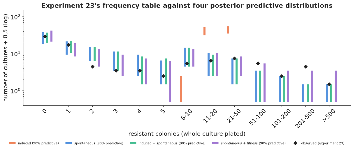
The comparison and the picture tell the same story.

• Induced + spontaneous adds nothing: its expected log predictive density is no better than the pure spontaneous model, the induced probability is pushed down to where it is irrelevant (upper bound above: a small fraction of one induced survivor per culture in experiment 23, next to about one mutation per culture), and its predictive distribution for experiment 23 (aqua) is the same as the spontaneous one (blue). On these data, with this prior, there is no sign of induced resistance - but the data cannot exclude a small amount of it either, which is Holmes et al.'s point.
• The tail is heavier than Luria-Delbrück. In experiment 23 the pure spontaneous model under-predicts the classes 51-100 and 201-500 (5 and 4 cultures observed, above its 90% intervals) and over-predicts the class "2": the data have more big jackpots and fewer small clones than a neutral Luria-Delbrück culture. The fitness extension (purple) covers 12 of the 13 classes; only 201-500 stays just above its interval. The induced model (orange) misses every class.
• The fitness model wins clearly on PSIS-LOO (22 units of elpd, three standard errors), with $\rho \approx 0.7$: taken literally, resistant mutants that grow about 40% faster than their sensitive parents. That literal reading is suspicious - there is no obvious reason for phage-resistant mutants to outgrow the wild type in phage-free broth. The same heavier tail arises if mutations happen preferentially early (Luria and Delbrück's own suggestion: a higher mutation rate in actively growing cells), if cultures were sometimes seeded with a pre-existing mutant, or if resistant cells clump or are counted differently on the plate. The fitness parameter is best read as a tail-shape parameter that the data demand, not as a measured growth rate.
• It matters for the rates. With the heavier tail, the jackpots no longer need a high mutation rate to explain them. The broth 10 ml series move down the most, and the broth-synthetic ratio becomes 0.72 (89% interval 0.45-1.10; 89% of draws below 1): a difference that may exist but is no longer clear. Conclusions about the rate and about media depend on getting the tail right.

fig, ax = plt.subplots(figsize=(10, 5))
plot_rates(ax, fits["spontaneous"], BLUE, "Luria-Delbrück (neutral mutants)", 0.15)
plot_rates(ax, fits["fitness"], PURPLE, "with differential growth (rho free)", -0.15)
log_ticks(ax, (0.2, 0.5, 1, 2))
ax.set_yticks(range(len(series)), [f"exp {n} ({'syn' if s.synthetic else 'broth'}, "
                                   f"{s.eps:.3g} plated)" for n, s in zip(names, series)])
ax.set(xlabel="mutation rate mu (x 1e-8 per cell per division, log)",
       title="How the tail model changes the per-experiment rates (89% intervals)")
ax.legend(fontsize=8);

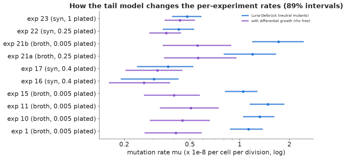
The synthetic series with whole or large-fraction plating (16, 17, 22, 23) barely move: their counts are dominated by zeros and small counts, which pin down $m$ whatever the tail. The 10 ml broth series with 0.5% plated (1, 10, 11, 15, 21b) drop by a factor of about 2.5-3: on their plates only large clones show up, so their rates are extrapolations through the tail. Experiment 21a (broth, 0.2 ml, mostly zeros) also halves, but for a different reason: it has little information of its own and is pulled along with the other broth series by the hierarchical prior. That is a lesson for design as much as for analysis: plating a tiny fraction of a huge culture makes the mutation rate hostage to the tail model.

#8 · Why the tail still matters

Mutation rates measured by fluctuation tests feed into questions with real consequences: how quickly resistance to an antibiotic will appear in an infection with $10^{10}$ bacteria, whether a clinical isolate is a mutator (rates 10-1000 times normal), whether a drug is mutagenic, how fast a tumour acquires a resistance mutation. In all of them, the quantity of interest is a rate and the data are dominated by rare, huge jackpots. This notebook showed the three ways that goes wrong and the fixes:

• Averages lie in a distribution with an $n^{-2}$ tail: the mean method overestimated every rate. Use the full likelihood (section 4) - here as a differentiable triangular solve, so the rate can sit inside any larger Bayesian model.
• Experimental details belong in the likelihood: the plated fraction changes the distribution (section 3), and ignoring it would bias the rate by orders of magnitude.
• Check the tail, and see what depends on it: the neutral model left experiment 23's jackpots under-predicted, and the rates for the 0.5%-plated series moved threefold when the tail was freed (section 7).

#Summary

• The fluctuation test distinguishes induced resistance (Poisson counts, variance = mean) from spontaneous mutation (jackpots, variance/mean of 5-250 in the 1943 data). Simulated growing cultures show why: a mutation's clone size depends exponentially on when it happened (sections 1-2).
• The Luria-Delbrück distribution has no closed form, but it is compound Poisson, and its Ma-Sandri-Sarkar recursion is one lower-triangular solve: exact, stable, differentiable in PyTensor, well under a millisecond for a few hundred terms. Partial plating, induced survivors and mutant fitness are changes of the clone-size probabilities, computed by quadrature (section 3).
• On experiment 23 the mean method overestimates the rate about fourfold; $p_0$, the MLE and the posterior agree on 1.1-1.2 mutations per culture. A simulation study shows the mean method's bias and scatter, $p_0$'s failure when $m$ is large and the MLE's reliability (section 4).
• PSIS-LOO and predictive checks of the largest culture reject induction on every series by a huge margin (section 5).
• With the full likelihood the rates come out 1.1-8 times lower than in 1943, and a threefold synthetic vs broth difference appears that the mean method had hidden (section 6).
• The data have a heavier tail than the neutral model: the Mandelbrot-Koch extension ($\rho \approx 0.7$) improves LOO by about 22 and fits experiment 23's classes, while an induced component adds nothing. The tail model moves the rates of the 0.5%-plated series threefold and shrinks the medium effect (section 7).

#Try it yourself

1. Two strains. The most common use of fluctuation analysis today is comparing a mutant (say a DNA-repair knockout) with the wild type. Simulate two series of 30 cultures with a threefold difference in $\mu$ and different final cell numbers, fit both in one model, and report the posterior of the fold change. How many cultures do you need for a 95% interval that excludes 1? Compare with the likelihood-ratio test in the rSalvador package (Zheng) if you have R.
2. Design. For a fixed number of plates, is it better to plate whole small cultures or a small fraction of large ones? Use the model of section 3 to compute the posterior width of $\log \mu$ for several $(\varepsilon, C)$ designs, with and without $\rho$ free. Section 7 suggests the answer changes when the tail is uncertain.
3. Other tails. Replace the fitness model by a mutation rate that decays as the culture saturates (more early mutations): the mixing density of $u$ becomes non-uniform, e.g. $\propto u^{\kappa}$ - only clone_matrix changes. Does it fit experiment 23 as well as $\rho$ does, and can LOO tell the two stories apart? Holmes et al. (2017) is a good companion.