Following one molecule at a time
A transcription factor has to find its binding sites among billions of base pairs of DNA. How long does it stay bound? What fraction of the molecules are bound at any moment? How fast do the free ones move, and does the crowded nucleus slow them down? Since about 2010 these questions are answered by single-particle tracking (SPT): tag the protein with a bright dye, excite so few molecules that each appears as an isolated spot, fit each spot's centre to a few tens of nanometres, and link the centres from frame to frame into tracks. A bound molecule jitters in place (with the chromatin it sits on); a free one jumps hundreds of nanometres per frame. The statistics of those jumps are the data.
They are treacherous data. Every position carries a localisation error of 20-40 nm, which for a bound molecule is as large as its real motion. The camera integrates each spot over the exposure, so a moving molecule is blurred. Tracks are short - a molecule bleaches or leaves the thin focal plane after a handful of frames, and fast molecules leave sooner. The standard workflow (compute a mean squared displacement curve, fit a straight line) mishandles all three. This notebook builds the exact likelihood instead and then uses it four ways: for single tracks, for a population of molecules in several states, for molecules that switch state inside a track, and to ask whether a motion is anomalous.
The plan
- Brownian motion, localisation error and motion blur
- The exact likelihood of a track, and a basis that makes it free
- One track at a time: the MSD fit versus the likelihood
- Data: RARA and a free control in living nuclei
- A population of states: bound and free (Spot-On style)
- Switching inside a track: a hidden Markov model that knows about localisation error
- Is it anomalous? Fractional Brownian motion and fake subdiffusion
import logging
import time
import warnings

import arviz as az
import matplotlib.pyplot as plt
import numpy as np
import pandas as pd
import pymc as pm
import pytensor
import pytensor.tensor as pt
import xarray as xr
from scipy import stats
from scipy.special import expit, logsumexp

from pymc_challenges import data

RANDOM_SEED = 57
rng = np.random.default_rng(RANDOM_SEED)
az.style.use("arviz-variat")
logging.getLogger("pymc").setLevel(logging.WARNING)
warnings.filterwarnings("ignore", category=FutureWarning)
warnings.filterwarnings("ignore", message="The effect of Potentials")
BLUE, ORANGE, AQUA, GREY, PURPLE, RED, INK = (
    "#2a78d6", "#eb6834", "#1baf7a", "#8a8a86", "#8c5ac8", "#c8384e", "#222222")
JAX = {"backend": "jax", "gradient_backend": "jax"}    # for the scan / Cholesky models (2-3x faster)
DT = 0.00748                                          # frame interval of the data (s)
print(f"PyMC {pm.__version__}, ArviZ {az.__version__}, PyTensor {pytensor.__version__}")


def fit(model, label, **kw):
    """Sample with nutpie, print time, divergences and worst r_hat / ESS of the named variables."""
    t0 = time.time()
    idata = pm.sample(model=model, random_seed=RANDOM_SEED, progressbar=False, **kw)
    names = kw.get("var_names") or list(idata.posterior.data_vars)
    rh = max(float(az.rhat(idata.posterior[v]).max()) for v in names)
    es = min(float(az.ess(idata.posterior[v]).min()) for v in names)
    print(f"{label}: {time.time() - t0:.0f} s, divergences {int(idata.sample_stats['diverging'].sum())}, "
          f"max r_hat {rh:.3f}, min ESS {es:.0f}")
    return idata
PyMC 6.3.2, ArviZ 1.3.0, PyTensor 3.3.2
1 · Brownian motion, localisation error and motion blur
A freely diffusing molecule in two dimensions takes independent Gaussian steps: over a time $\Delta t$ each coordinate moves by $\mathcal N(0, 2D\Delta t)$, where $D$ is the diffusion coefficient (µm²/s). Its mean squared displacement grows linearly, $\text{MSD}(\tau) = \langle |r(t+\tau) - r(t)|^2\rangle = 4D\tau$ in 2-D, and the MSD curve of a track is the standard summary.
Two things stand between the molecule and the recorded positions.
- Static localisation error. Each recorded position is the true one plus $\mathcal N(0, \sigma^2)$ per coordinate, independently from frame to frame; $\sigma$ is set by the number of photons and the background (typically 20-40 nm).
- Motion blur. The camera records the average position over the exposure, not a snapshot. Averaging a Brownian path over a window shrinks its variance. Berglund (2010) summarised any exposure profile by one number, $R$ ($R = 1/6$ for a continuous exposure over the whole frame, $R \approx 0$ for a short stroboscopic flash).
For the observed displacements $\Delta_k = y_{k+1} - y_k$ of one coordinate this gives (Berglund 2010, eq. 7; Michalet 2010)
$$\operatorname{Var}(\Delta_k) = 2D\Delta t\,(1 - 2R) + 2\sigma^2, \qquad \operatorname{Cov}(\Delta_k, \Delta_{k+1}) = 2D\Delta t\,R - \sigma^2, \qquad \operatorname{Cov}(\Delta_k, \Delta_{k+j}) = 0 \ (j \ge 2).$$
The same error $e_{k+1}$ enters $\Delta_k$ with a plus sign and $\Delta_{k+1}$ with a minus sign, so successive displacements are negatively correlated - a jump "out" by error is followed by a jump "back". The MSD curve becomes $4D\tau + 4\sigma^2 - 8DR\Delta t$: a line with an offset. We simulate this at the scales of the data below: a bound molecule ($D = 0.03$ µm²/s), a free one ($D = 3$ µm²/s), $\sigma = 30$ nm, $\Delta t = 7.48$ ms. The simulator follows the true path on 30 sub-steps per frame and averages it over the exposure.
def simulate_track(n, D, sigma, rng, dt=DT, exposure=1.0, sub=30):
    """n observed 2-D positions: Brownian path averaged over `exposure` x dt of each frame + error."""
    h = dt / sub
    path = np.cumsum(rng.normal(0, np.sqrt(2 * D * h), size=(n * sub, 2)), axis=0).reshape(n, sub, 2)
    m = max(1, int(round(exposure * sub)))
    return path[:, :m].mean(axis=1) + rng.normal(0, sigma, size=(n, 2))


def msd_curve(track, max_lag):
    return np.array([np.mean(np.sum((track[k:] - track[:-k]) ** 2, axis=1)) for k in range(1, max_lag + 1)])


def rho1(D, sigma, R, dt=DT):
    """Lag-1 correlation of successive displacements (one coordinate)."""
    return (2 * D * dt * R - sigma**2) / (2 * D * dt * (1 - 2 * R) + 2 * sigma**2)


rng1 = np.random.default_rng(1)
fig, axes = plt.subplots(1, 3, figsize=(15, 4.4))
ax = axes[0]
for D, col, lab in [(0.03, BLUE, "bound, D = 0.03"), (3.0, ORANGE, "free, D = 3")]:
    tr = simulate_track(60, D, 0.03, rng1, exposure=0.03)
    ax.plot(tr[:, 0] - tr[0, 0], tr[:, 1] - tr[0, 1], "-o", ms=2.5, lw=0.8, color=col, label=lab)
ax.set(xlabel="x (µm)", ylabel="y (µm)", title="60 frames (0.45 s), σ = 30 nm")
ax.set_aspect("equal", adjustable="datalim")
ax.legend(fontsize=8)

ax = axes[1]
lags = np.arange(1, 21)
for sigma, col in [(0.0, GREY), (0.03, BLUE), (0.05, PURPLE)]:
    m = np.mean([msd_curve(simulate_track(200, 0.03, sigma, rng1, exposure=0.03), 20)
                 for _ in range(200)], axis=0)
    ax.plot(lags * DT * 1e3, m * 1e3, "o", ms=3, color=col, label=f"σ = {sigma * 1e3:.0f} nm")
    ax.plot(lags * DT * 1e3, (4 * 0.03 * lags * DT + 4 * sigma**2) * 1e3, lw=1, color=col)
ax.set(xlabel="lag τ (ms)", ylabel="MSD (10⁻³ µm²)", title="Bound molecule: MSD = 4Dτ + 4σ²",
       ylim=(0, None))
ax.legend(fontsize=8)

ax = axes[2]
x_grid = np.logspace(-2, 1.5, 100)                       # sigma^2 / (D dt)
for R, col, lab, expo in [(0.0, BLUE, "strobed flash (R ≈ 0)", 0.03), (1 / 6, ORANGE, "full-frame exposure (R = 1/6)", 1.0)]:
    ax.plot(x_grid, rho1(1.0, np.sqrt(x_grid * DT), R), color=col, label=lab)
    for xv in [0.03, 0.3, 3, 30]:
        sig = np.sqrt(xv * 1.0 * DT)
        d = np.concatenate([np.diff(simulate_track(400, 1.0, sig, rng1, exposure=expo), axis=0)
                            for _ in range(25)])
        ax.plot(xv, np.corrcoef(d[:-1, 0], d[1:, 0])[0, 1], "o", color=col, ms=5)
ax.axhline(0, color=GREY, lw=0.8)
ax.set(xscale="log", xlabel="σ² / (D Δt)   (error relative to motion per frame)",
       ylabel="corr(Δₖ, Δₖ₊₁)", title="Successive displacements anticorrelate", ylim=(-0.55, 0.3))
ax.legend(fontsize=8, loc="lower left");
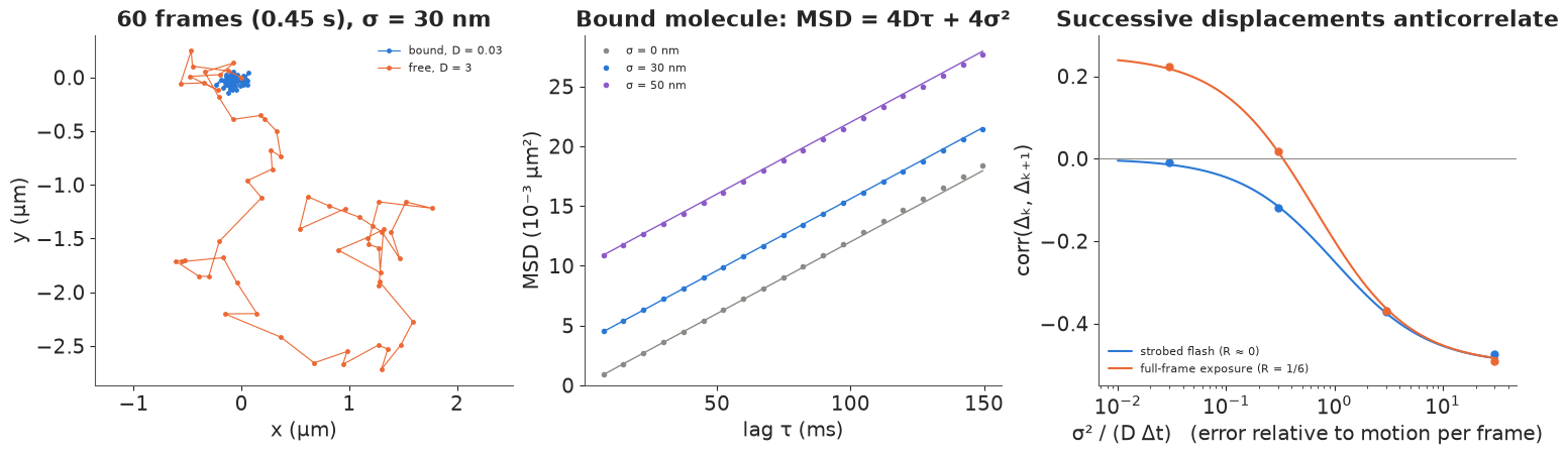
Left: in 60 frames the bound molecule stays within about 0.1 µm, while the free one wanders 3 µm. Middle: averaged over 200 simulated tracks, the MSD of the bound molecule is a straight line whose intercept is $4\sigma^2$: with $\sigma = 30$ nm the offset equals the diffusive growth over $\sigma^2/D = 30$ ms, four frames. For a bound molecule at 30-50 nm error, most of the first MSD points is error. Right: the lag-1 correlation of successive displacements (lines: the formula; dots: simulations) depends on one number, the error relative to the motion per frame, $\sigma^2 / (D\Delta t)$. With a short flash it runs from 0 (motion dominates) to $-1/2$ (error dominates). With full-frame exposure blur adds a positive correlation of up to $+1/4$ (an averaged path is smoother), and the two curves merge once error dominates. For the data below a bound molecule has $\sigma^2/(D\Delta t) \approx 4$ (correlation about $-0.4$), a free one about 0.04.
2 · The exact likelihood of a track, and a basis that makes it free
Stack the $m = n - 1$ displacements of one coordinate into a vector $\Delta$. It is Gaussian with mean zero and the tridiagonal Toeplitz covariance $\Sigma$ above: diagonal $a = 2D\Delta t(1-2R)
- 2\sigma^2$, off-diagonal $b = 2D\Delta tR - \sigma^2$. That is the covariance of a moving average of order one (MA(1)), and $x$ and $y$ are independent. Fitting a line to an MSD curve throws most of this structure away (and treats strongly correlated MSD points as independent); the likelihood uses all of it.
One could hand $\Sigma$ to pm.MvNormal, one track at a time. There is a much better way. Every
tridiagonal Toeplitz matrix has the same eigenvectors, the discrete sine basis
$Q_{ij} = \sqrt{2/(m+1)}\,\sin(ij\pi/(m+1))$, with eigenvalues $a + 2b\cos(j\pi/(m+1))$. So if we
rotate each track once, in NumPy, $u = Q\Delta$, the $m$ coefficients are independent
Gaussians with variances
$$v_j = 2D\Delta t\,\big[1 - 2R(1 - c_j)\big] + 2\sigma^2 (1 - c_j), \qquad c_j = \cos\frac{j\pi}{m+1}.$$
This is the likelihood of a track as a plain pm.Normal on precomputed numbers: no matrices, no
scan, any number of tracks of any lengths in one vector. It also reads like a spectrum: slow
modes ($c_j \approx 1$) have variance $2D\Delta t$ and see only diffusion; fast modes ($c_j
\approx -1$) have variance $2D\Delta t(1-4R) + 4\sigma^2$ and carry the localisation error.
A track of $m$ displacements has only $m$ modes to split between the two - the root of the
$D$-$\sigma$ trade-off below. And one more consequence: $\sigma^2$ and $R$ enter only through
$\sigma^2 - 2DR\Delta t$, so blur and localisation error cannot be separated from tracks alone
- $\sigma$ fitted with $R = 0$ is an effective error (smaller than the true one when there is blur). We check the rotation against the dense Gaussian first.
def dst_basis(m):
    """Eigenvectors (rows) and cosines of every m x m tridiagonal Toeplitz matrix."""
    j = np.arange(1, m + 1)
    return np.sqrt(2 / (m + 1)) * np.sin(np.outer(j, j) * np.pi / (m + 1)), np.cos(j * np.pi / (m + 1))


def mode_var(D, sigma, c, R=0.0, dt=DT):
    return 2 * D * dt * (1 - 2 * R * (1 - c)) + 2 * sigma**2 * (1 - c)


m_chk, D_chk, s_chk, R_chk = 12, 0.5, 0.03, 1 / 6
Sigma = (np.diag(np.full(m_chk, 2 * D_chk * DT * (1 - 2 * R_chk) + 2 * s_chk**2))
         + (2 * D_chk * DT * R_chk - s_chk**2) * (np.eye(m_chk, k=1) + np.eye(m_chk, k=-1)))
Q, c = dst_basis(m_chk)
x_chk = rng.multivariate_normal(np.zeros(m_chk), Sigma)
print(f"dense MvNormal logpdf {stats.multivariate_normal(np.zeros(m_chk), Sigma).logpdf(x_chk):.10f}")
print(f"sine-basis sum       {stats.norm(0, np.sqrt(mode_var(D_chk, s_chk, c, R_chk))).logpdf(Q @ x_chk).sum():.10f}")


def pack_tracks(tracks, cap=None):
    """Rotate every track: returns summed squared coefficients (x and y), cosines and track index."""
    z2, cc, idx = [], [], []
    for i, t in enumerate(tracks):
        d = np.diff(t[:cap], axis=0)
        Qm, cm = dst_basis(len(d))
        z2.append(((Qm @ d) ** 2).sum(axis=1))
        cc.append(cm)
        idx.append(np.full(len(d), i))
    return np.concatenate(z2), np.concatenate(cc), np.concatenate(idx)
dense MvNormal logpdf 14.7909033297
sine-basis sum       14.7909033297
Because $x$ and $y$ share the variance $v_j$, each mode contributes a $\chi^2$ with two degrees of freedom: $\log p = -\log(2\pi v_j) - (u_{x,j}^2 + u_{y,j}^2)/(2 v_j)$. The figure shows the mode variances for a bound molecule and the empirical "periodogram" (the squared coefficients, averaged over 500 simulated tracks of 30 positions).
fig, axes = plt.subplots(1, 2, figsize=(12, 4.2))
m30 = 29
Q30, c30 = dst_basis(m30)
jj = np.arange(1, m30 + 1)
for ax, D, title in [(axes[0], 0.03, "bound molecule, D = 0.03 µm²/s"), (axes[1], 3.0, "free molecule, D = 3 µm²/s")]:
    for sigma, col in [(0.0, GREY), (0.03, BLUE), (0.05, PURPLE)]:
        sims = np.array([np.diff(simulate_track(30, D, sigma, rng1, exposure=0.03), axis=0) for _ in range(500)])
        pg = np.mean((np.einsum("ij,njk->nik", Q30, sims) ** 2).mean(axis=2), axis=0)
        ax.plot(jj, pg / (2 * D * DT), "o", ms=3, color=col)
        ax.plot(jj, mode_var(D, sigma, c30) / (2 * D * DT), color=col, lw=1, label=f"σ = {sigma * 1e3:.0f} nm")
    ax.set(xlabel="mode j (slow → fast)", ylabel="variance / (2DΔt)", title=title, yscale="log" if D < 1 else "linear")
    ax.legend(fontsize=8)
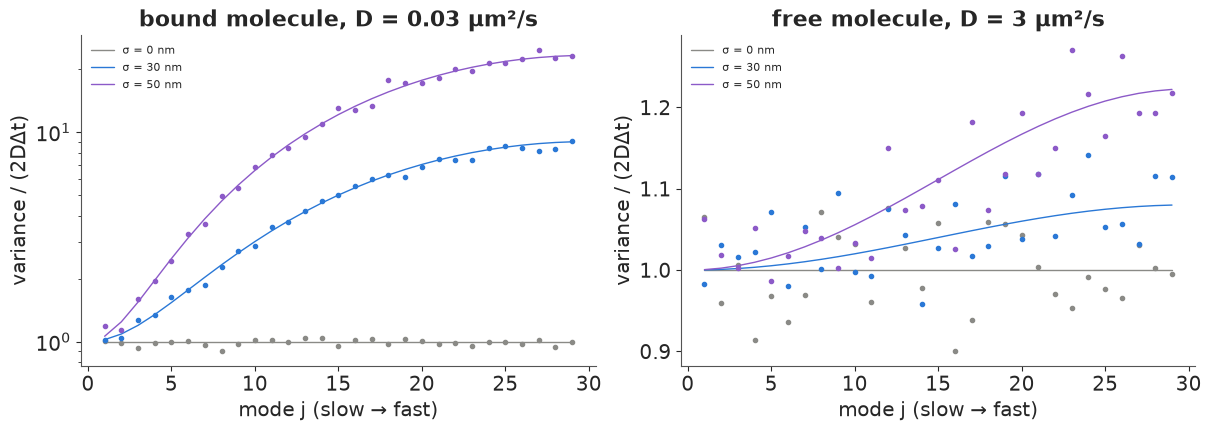
The dots (simulation) sit on the lines (formula). For the bound molecule the fast modes carry 9 times ($\sigma = 30$ nm) and 23 times ($\sigma = 50$ nm) the variance of the slow ones: the slow end of the spectrum is where $D$ is measured, and a track needs enough slow modes - enough length - for that. For the free molecule the error lifts the fast modes by at most 8% and 22%, within the scatter of 500 tracks: at $D = 3$ µm²/s localisation error barely matters and $\sigma$ will be hard to learn from free molecules.
3 · One track at a time: the MSD fit versus the likelihood
First a single short track (11 positions, a typical length in the data) and a long one (101 positions) of the same bound molecule, $D = 0.03$ µm²/s and $\sigma = 30$ nm, each with its own $D$ and $\sigma$. Priors: $\log D \sim \mathcal N(\log 0.1, 2)$ (from 0.002 to 5 µm²/s within two sd, bound to free), $\log\sigma \sim \mathcal N(\log 0.03, 1)$ (a factor of 2.7 around 30 nm).
def per_track_model(tracks, R=0.0):
    z2, cc, idx = pack_tracks(tracks)
    with pm.Model(coords={"track": np.arange(len(tracks))}) as model:
        logD = pm.Normal("logD", np.log(0.1), 2.0, dims="track")
        log_sigma = pm.Normal("log_sigma", np.log(0.03), 1.0, dims="track")
        v = mode_var(pt.exp(logD)[idx], pt.exp(log_sigma)[idx], cc, R)
        pm.Potential("lik", pt.sum(-pt.log(2 * np.pi * v) - z2 / (2 * v)))
    return model


rng3 = np.random.default_rng(3)
track_short = simulate_track(11, 0.03, 0.03, rng3, exposure=0.03)
track_long = simulate_track(101, 0.03, 0.03, rng3, exposure=0.03)
idata_short = fit(per_track_model([track_short]), "11 positions")
idata_long = fit(per_track_model([track_long]), "101 positions")

fig, axes = plt.subplots(1, 2, figsize=(12, 4.4))
ax = axes[0]
for idata_, col, lab in [(idata_short, ORANGE, "11 positions"), (idata_long, BLUE, "101 positions")]:
    ax.plot(np.exp(idata_.posterior["logD"].values.ravel()), np.exp(idata_.posterior["log_sigma"].values.ravel()) * 1e3,
            ".", ms=1.5, alpha=0.3, color=col, label=lab)
ax.plot(0.03, 30, "*", ms=14, color=INK, label="truth")
ax.set(xscale="log", xlabel="D (µm²/s)", ylabel="σ (nm)", title="Posterior draws: the D-σ trade-off", xlim=(1e-3, 0.3))
ax.legend(handles=[plt.Line2D([], [], ls="", marker="o", color=ORANGE, label="11 positions"),
                   plt.Line2D([], [], ls="", marker="o", color=BLUE, label="101 positions"),
                   plt.Line2D([], [], ls="", marker="*", ms=10, color=INK, label="truth")], fontsize=8)
ax = axes[1]
for tr, col, lab in [(track_short, ORANGE, "11 positions"), (track_long, BLUE, "101 positions")]:
    mm = msd_curve(tr, min(10, len(tr) - 1))
    ax.plot(np.arange(1, len(mm) + 1) * DT * 1e3, mm * 1e3, "o-", ms=3, lw=0.8, color=col, label=lab)
lg = np.arange(0, 11)
ax.plot(lg * DT * 1e3, (4 * 0.03 * lg * DT + 4 * 0.03**2) * 1e3, "--", color=INK, lw=1, label="truth 4Dτ + 4σ²")
ax.set(xlabel="lag τ (ms)", ylabel="MSD (10⁻³ µm²)", title="Their MSD curves", ylim=(0, None))
ax.legend(fontsize=8)
for lab, idata_ in [("11", idata_short), ("101", idata_long)]:
    Dd = np.exp(idata_.posterior["logD"].values.ravel())
    sd = np.exp(idata_.posterior["log_sigma"].values.ravel())
    print(f"{lab:>3} positions: D 89% interval {np.quantile(Dd, 0.055):.3f}-{np.quantile(Dd, 0.945):.3f} µm²/s, "
          f"sigma {np.quantile(sd, 0.055) * 1e3:.0f}-{np.quantile(sd, 0.945) * 1e3:.0f} nm, "
          f"corr(log D, log sigma) = {np.corrcoef(np.log(Dd), np.log(sd))[0, 1]:.2f}")
11 positions: 2 s, divergences 0, max r_hat 1.003, min ESS 959
101 positions: 0 s, divergences 0, max r_hat 1.001, min ESS 2222
 11 positions: D 89% interval 0.037-0.255 µm²/s, sigma 7-45 nm, corr(log D, log sigma) = -0.57
101 positions: D 89% interval 0.015-0.039 µm²/s, sigma 27-34 nm, corr(log D, log sigma) = -0.50
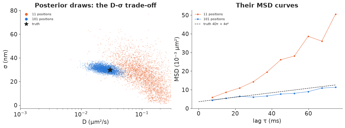
Left: the posterior of the long track is a small blob around the truth. The short track's is a long diagonal ridge (correlation $-0.57$ between $\log D$ and $\log\sigma$): a bit more diffusion and a bit less error explain ten displacements equally well. The data pin down roughly $2D\Delta t + 2\sigma^2$, not the split. This particular short track also happens to wander more than a typical one (its MSD curve, right, climbs far above the truth), so its 89% interval for $D$, 0.037-0.255 µm²/s, misses the true 0.03. That is what 89% intervals do about one time in nine; the 200-track check below measures how often. Its $\sigma$ interval (7-45 nm) says the track itself carries little information on the error. The long track gives $D$ 0.015-0.039 and $\sigma$ 27-34 nm.
Two hundred short tracks: three estimators
Now 200 tracks of 11 positions each, with $D$ spread log-normally around 0.05 µm²/s (from bound to slow) and $\sigma = 30$ nm, all fitted in one model (each track its own $D$ and $\sigma$; 400 parameters, one vector of modes). We compare the posterior median of $D$ with two MSD estimators in everyday use: $\hat D_1 = \text{MSD}(\Delta t)/4\Delta t$ (the first point alone, which ignores the error) and a least-squares line through the first four MSD points, $\text{MSD} = 4D\tau + \text{offset}$ (which allows for it; Michalet 2010 shows that few points are best).
rng3b = np.random.default_rng(33)
n_sim = 200
D_true = np.exp(rng3b.normal(np.log(0.05), 1.0, n_sim))
sim_tracks = [simulate_track(11, d, 0.03, rng3b, exposure=0.03) for d in D_true]
idata_200 = fit(per_track_model(sim_tracks), "200 tracks, 400 parameters")

D_bayes = np.exp(idata_200.posterior["logD"].median(("chain", "draw")).values)
lo, hi = np.exp(idata_200.posterior["logD"].quantile([0.055, 0.945], dim=("chain", "draw")).values)
D_msd1 = np.array([msd_curve(t, 1)[0] / (4 * DT) for t in sim_tracks])
X_ls = np.c_[4 * DT * np.arange(1, 5), np.ones(4)]
D_line = np.array([np.linalg.lstsq(X_ls, msd_curve(t, 4), rcond=None)[0][0] for t in sim_tracks])
print(f"89% intervals covering the true D: {np.mean((D_true > lo) & (D_true < hi)):.0%}")
for lab, est in [("MSD(1)/4dt", D_msd1), ("4-point MSD line", D_line), ("posterior median", D_bayes)]:
    ok = est > 0
    print(f"{lab:>17}: median ratio to truth {np.median(est / D_true):5.2f}, "
          f"non-positive {np.mean(~ok):4.0%}, rms log error (positive ones) "
          f"{np.sqrt(np.mean(np.log(est[ok] / D_true[ok]) ** 2)):.2f}")

fig, axes = plt.subplots(1, 3, figsize=(15, 4.4), sharex=True, sharey=True)
for ax, (lab, est, col) in zip(axes, [("MSD(Δt) / 4Δt", D_msd1, GREY), ("line through 4 MSD points", D_line, PURPLE),
                                      ("posterior median (exact likelihood)", D_bayes, BLUE)]):
    ok = est > 0
    ax.plot(D_true[ok], est[ok], "o", ms=3.5, color=col, alpha=0.7)
    ax.plot(D_true[~ok], np.full((~ok).sum(), 1.2e-3), "v", ms=4, color=RED, label=f"≤ 0: {(~ok).sum()} tracks")
    if lab.startswith("posterior"):
        ax.vlines(D_true, lo, hi, color=col, lw=0.5, alpha=0.4)
    ax.plot([1e-3, 3], [1e-3, 3], color=INK, lw=0.8)
    ax.axvline(0.03**2 / DT, color=GREY, ls=":", lw=1)
    ax.set(xscale="log", yscale="log", xlabel="true D (µm²/s)", title=lab, xlim=(1e-3, 2), ylim=(1e-3, 3))
    if (~ok).any():
        ax.legend(fontsize=8, loc="upper left")
axes[0].set_ylabel("estimated D (µm²/s)");
200 tracks, 400 parameters: 2 s, divergences 0, max r_hat 1.008, min ESS 1768
89% intervals covering the true D: 91%
       MSD(1)/4dt: median ratio to truth  2.97, non-positive   0%, rms log error (positive ones) 1.43
 4-point MSD line: median ratio to truth  0.81, non-positive  13%, rms log error (positive ones) 1.06
 posterior median: median ratio to truth  1.08, non-positive   0%, rms log error (positive ones) 0.66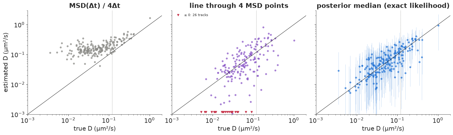
- MSD$(\Delta t)/4\Delta t$ estimates $D + \sigma^2/\Delta t$, not $D$: for every bound molecule it reports about 0.1-0.2 µm²/s whatever the truth (median 3 times too large). The dotted line marks $D = \sigma^2/\Delta t = 0.12$ µm²/s, where the error per frame equals the motion; below it this estimator measures the microscope, not the molecule.
- The four-point line removes the offset on average (median ratio 0.8) but is wildly noisy: 26 of 200 tracks (13%) get a zero or negative $D$, and the rest scatter over two decades (rms error 1.06 in $\log D$). Four correlated MSD points of an 11-position track are not four independent measurements.
- The exact likelihood is close to unbiased (median ratio 1.08), has the smallest error (rms 0.66 in $\log D$), never goes negative, and its 89% intervals cover the truth for 91% of tracks - honest uncertainty, wide where the track is short and the molecule slow.
All 200 tracks with 400 parameters sampled in a couple of seconds, because the likelihood is one
vectorised Normal over precomputed modes.
4 · Data: RARA and a free control in living nuclei
The saSPT package (Heckert, Dahal, Tjian & Darzacq 2022) ships two real datasets as examples: tracks of RARA-HaloTag, a nuclear receptor that binds DNA, and of HaloTag-NLS, the bare tag with a nuclear localisation signal, which has nothing to bind and should diffuse freely. Both were imaged in the nuclei of U2OS cells at 7.48 ms per frame with 160 nm pixels, and the package's settings give a focal depth of 0.7 µm. Molecules are photoactivated sparsely, so each region (one nucleus) contributes thousands of short tracks. We keep two RARA nuclei and all eleven control nuclei, frames from 1000 on (as the package's examples do, after the initial dense phase). The file also carries each localisation's fitted error.
data.describe("heckert2022_spt")
tracks_df = data.load("heckert2022_spt")
tracks_df.head()
heckert2022_spt: Single-molecule tracks in nuclei of live human U2OS cells, 7.48 ms per frame (package settings: 0.16 um pixels, 0.7 um focal depth), one row per localisation: condition (rara = RARA-HaloTag, the retinoic acid receptor alpha; nls = HaloTag-NLS, a free control), region (one nucleus / movie), track (trajectory id within the region), frame, x_um, y_um, loc_err_um (mean of the fitted x and y localisation errors). 34,401 RARA and 46,990 NLS localisations, tracks of 1 to 242 positions.
  source: Example data of the saSPT package (github.com/alecheckert/saspt, examples/, MIT licence), described with the method in Heckert, Dahal, Tjian & Darzacq (2022), Recovering mixtures of fast-diffusing states from short single-particle trajectories, eLife 11:e70169. EXTRACTED from 13 of the 22 example CSVs (u2os_rara_ht_7.48ms/region_4 and region_5; u2os_ht_nls_7.48ms/region_0..10; the URL is one of them), frames >= 1000, positions converted from pixels (0.16 um) to um, so keep the cached file in data/.
  url:    https://raw.githubusercontent.com/alecheckert/saspt/main/examples/u2os_rara_ht_7.48ms/region_4_7ms_trajs.csv
| condition | region | track | frame | x_um | y_um | loc_err_um | |
|---|---|---|---|---|---|---|---|
| 0 | rara | 4 | 2771 | 1001 | 5.7741 | 1.5083 | 0.0296 |
| 1 | rara | 4 | 2772 | 1001 | 4.6857 | 19.3899 | 0.0382 |
| 2 | rara | 4 | 2773 | 1000 | 15.5410 | 14.9514 | 0.0204 |
| 3 | rara | 4 | 2773 | 1001 | 15.3993 | 15.0375 | 0.0126 |
| 4 | rara | 4 | 2773 | 1002 | 15.4920 | 14.9059 | 0.0146 |
track_len = tracks_df.groupby(["condition", "region", "track"]).size().rename("n").reset_index()
summary = track_len.groupby("condition").agg(
    nuclei=("region", "nunique"), tracks=("n", "size"), singletons=("n", lambda n: np.mean(n == 1)),
    median_len_ge2=("n", lambda n: np.median(n[n >= 2])), max_len=("n", "max"))
summary["localisation error (nm, median)"] = tracks_df.groupby("condition")["loc_err_um"].median() * 1e3
print(summary.round(2).to_string())


def get_tracks(cond, min_len=2):
    """Lists of (n, 2) position arrays (µm) and of reported localisation errors, and region labels."""
    out, err, reg = [], [], []
    sub = tracks_df[tracks_df.condition == cond].sort_values(["region", "track", "frame"])
    for (r, _), g in sub.groupby(["region", "track"], sort=False):
        if len(g) >= min_len:
            out.append(g[["x_um", "y_um"]].to_numpy())
            err.append(g["loc_err_um"].to_numpy())
            reg.append(r)
    return out, err, np.array(reg)


rara_tracks, rara_err, rara_region = get_tracks("rara")
nls_tracks, _, nls_region = get_tracks("nls")
first_jump = {c: np.array([np.hypot(*(t[1] - t[0])) for t in trs]) for c, trs in [("rara", rara_tracks), ("nls", nls_tracks)]}
lengths = {"rara": np.array([len(t) for t in rara_tracks]), "nls": np.array([len(t) for t in nls_tracks])}
print(f"tracks with >= 2 positions: RARA {len(rara_tracks)}, NLS {len(nls_tracks)}")
for c, trs in [("rara", rara_tracks), ("nls", nls_tracks)]:
    all_j = np.concatenate([np.hypot(*np.diff(t, axis=0).T) for t in trs])
    print(f"{c}: {len(all_j)} jumps, longest {all_j.max():.3f} µm, 99.9% quantile {np.quantile(all_j, 0.999):.3f} µm")
           nuclei  tracks  singletons  median_len_ge2  max_len  localisation error (nm, median)
condition
nls            11   19755        0.64             3.0      211                             34.0
rara            2    7873        0.52             4.0      242                             20.2
tracks with >= 2 positions: RARA 3770, NLS 7166
rara: 26528 jumps, longest 1.188 µm, 99.9% quantile 1.122 µm
nls: 27235 jumps, longest 1.975 µm, 99.9% quantile 1.822 µm
fig, axes = plt.subplots(1, 3, figsize=(15, 4.4))
ax = axes[0]
sel = [t for t in rara_tracks if len(t) >= 15][:40]
for t in sel:
    jumps = np.hypot(*np.diff(t, axis=0).T)
    ax.plot(t[:, 0], t[:, 1], "-", lw=0.8, color=ORANGE if np.median(jumps) > 0.15 else BLUE)
ax.set(xlabel="x (µm)", ylabel="y (µm)", title="40 RARA tracks (≥ 15 positions), one nucleus")
ax.set_aspect("equal", adjustable="datalim")
ax = axes[1]
bins = np.linspace(0, 1.6, 81)
for c, col, lab in [("rara", BLUE, "RARA-HaloTag"), ("nls", ORANGE, "HaloTag-NLS")]:
    ax.hist(first_jump[c], bins=bins, density=True, histtype="step", lw=1.5, color=col, label=lab)
ax.set(xlabel="first jump of each track (µm in 7.48 ms)", ylabel="density", title="Jump lengths")
ax.legend(fontsize=8)
ax = axes[2]
for c, col, lab in [("rara", BLUE, "RARA-HaloTag"), ("nls", ORANGE, "HaloTag-NLS")]:
    L = lengths[c]
    ns = np.arange(2, 61)
    ax.plot(ns, [(L >= n).mean() for n in ns], "o-", ms=2.5, lw=0.8, color=col, label=lab)
ax.set(yscale="log", xlabel="track length n (positions)", ylabel="fraction of tracks ≥ n",
       title="Track lengths (tracks with ≥ 2 positions)")
ax.legend(fontsize=8);
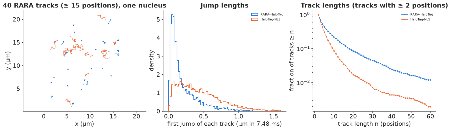
The table and figure show what makes real SPT data hard. Half or more of all tracks are single localisations (52% for RARA, 64% for the control) with no displacement at all, and a typical track has 3-4 positions. The reported localisation errors are 20 nm (RARA) and 34 nm (control, whose spots are dimmer) - the same order as a bound molecule's motion per frame. Left: 40 RARA tracks of one nucleus, coloured by their median jump: compact knots (bound) and open wanderings (free). Middle: RARA's first jumps have a sharp peak at about 50 nm - bound molecules, a peak made mostly of localisation error - and a long tail; the control has no peak and a broad distribution out to 1.5 µm. Right: control tracks are shorter (0.6% reach 30 positions, against 5% for RARA): a fast molecule leaves the 0.7 µm focal slice within a few frames.
One more thing hides in the printed jump ranges: no RARA jump is longer than 1.19 µm and no control jump longer than 1.98 µm. The tracking software only links spots within a search radius; a molecule that jumped further starts a new track. For the states fitted below this truncation is negligible (a $D = 6$ µm²/s molecule jumps more than 1.2 µm in 0.06% of frames), but it would bias any faster state.
5 · A population of states: bound and free (Spot-On style)
The classic analysis of such data (Spot-On, Hansen et al. 2018) treats every track as coming from one of a few states with their own $D$ - "bound" and "free", perhaps a third - and estimates the fraction of molecules in each. With the sine-basis likelihood this is a mixture over whole tracks: track $i$ with modes $u_{ij}$ has
$$p(\text{track}_i) = \sum_s w_s\, p(n_i \mid s) \prod_j \mathcal N_2\big(u_{ij} \mid 0, v_j(D_s, \sigma)\big),$$
with $\sigma$ shared (an effective error, $R = 0$; the exposure profile of these movies is not in the repository). The factor $p(n_i \mid s)$ is where the out-of-focus bias lives. A molecule is lost when it bleaches, blinks or leaves the 0.7 µm focal slice, and a free molecule leaves the slice far sooner than a bound one. So long tracks are mostly bound, and any analysis that keeps only "good" long tracks under-counts the free state. Spot-On corrects for this with a calculated escape probability; here we let the data speak and give each state its own per-frame survival probability $q_s$: $p(n \mid s) = (1 - q_s)\, q_s^{\,n-2}$ for $n \ge 2$ positions. The weights $w_s$ are then the state fractions among tracks at their first jump, which is what the first jumps in the middle panel above show. To keep the model quick, only the first 20 positions of each track enter the likelihood of the displacements (the length term uses the full length).
Priors: $\log D_s$ normal with sd 1.5 around 0.03, 0.8 (for three states) and 3 µm²/s, with the ordered transform (no label switching); $w \sim$ Dirichlet(2, ...); $\sigma \sim$ LogNormal($\log 0.03$, 0.5); $q_s \sim$ Beta(2, 2).
CAP = 20


def mixture_model(tracks, lens, K, use_length=True, cap=CAP):
    z2, cc, idx = pack_tracks(tracks, cap)
    mu0 = {1: [np.log(3.0)], 2: [np.log(0.03), np.log(3.0)], 3: [np.log(0.03), np.log(0.8), np.log(3.0)]}[K]
    with pm.Model(coords={"state": np.arange(K)}) as model:
        logD = pm.Normal("logD", mu0, 1.5, dims="state",
                         transform=pm.distributions.transforms.ordered if K > 1 else None)
        w = pm.Dirichlet("w", np.full(K, 2.0), dims="state")
        sigma = pm.LogNormal("sigma", np.log(0.03), 0.5)
        pm.Deterministic("D", pt.exp(logD), dims="state")
        v = 2 * pt.exp(logD)[None] * DT + 2 * sigma**2 * (1 - cc)[:, None]           # modes x states
        lp_mode = -pt.log(2 * np.pi * v) - z2[:, None] / (2 * v)
        lp_track = pt.zeros((len(tracks), K))
        lp_track = pt.inc_subtensor(lp_track[idx], lp_mode)
        if use_length:
            q = pm.Beta("q", 2.0, 2.0, dims="state")
            lp_track = lp_track + pt.log1p(-q)[None] + (lens[:, None] - 2) * pt.log(q)[None]
        pm.Potential("lik", pt.logsumexp(pt.log(w)[None] + lp_track, axis=1).sum())
    return model


def mixture_track_loglik(idata, tracks, lens, cap=CAP, n_draws=400):
    """Per-track log-likelihood (draws x tracks) and state responsibilities, in NumPy."""
    z2, cc, idx = pack_tracks(tracks, cap)
    post = az.extract(idata, var_names=["D", "w", "sigma", "q"], num_samples=n_draws, random_seed=RANDOM_SEED)
    D, w, s, q = (post[v].values for v in ["D", "w", "sigma", "q"])
    D, w, q = D.reshape(-1, n_draws).T, w.reshape(-1, n_draws).T, q.reshape(-1, n_draws).T
    K, N = D.shape[1], len(tracks)
    ll = np.zeros((n_draws, N))
    resp = np.zeros((N, K))
    for i in range(n_draws):
        v = 2 * D[i][None] * DT + 2 * s[i] ** 2 * (1 - cc)[:, None]
        lpm = -np.log(2 * np.pi * v) - z2[:, None] / (2 * v)
        lpt = np.stack([np.bincount(idx, lpm[:, k], minlength=N) for k in range(K)], axis=1)
        lpt += np.log1p(-q[i])[None] + (lens[:, None] - 2) * np.log(q[i])[None] + np.log(w[i])[None]
        ll[i] = logsumexp(lpt, axis=1)
        resp += np.exp(lpt - ll[i][:, None]) / n_draws
    return ll, resp


def loo_from(ll, name="track"):
    tree = xr.DataTree.from_dict({
        "posterior": xr.Dataset({"dummy": (("chain", "draw"), np.zeros((1, ll.shape[0])))}),
        "log_likelihood": xr.Dataset({name: (("chain", "draw", name), ll[None])})})
    return az.loo(tree, var_name=name, pointwise=True)


lens_rara = lengths["rara"]
mix = {}
for K in (2, 3):
    mix[K] = fit(mixture_model(rara_tracks, lens_rara, K), f"RARA, {K} states")
    print(az.summary(mix[K], var_names=["D"], round_to=3).iloc[:, :4].to_string())
    print(az.summary(mix[K], var_names=["w"], round_to=3).iloc[:, :4].to_string())
    print(az.summary(mix[K], var_names=["q"], round_to=3).iloc[:, :4].to_string())
    print(az.summary(mix[K], var_names=["sigma"], round_to=4).iloc[:, :4].to_string())
RARA, 2 states: 6 s, divergences 0, max r_hat 1.003, min ESS 779
       mean     sd  eti89_lb  eti89_ub
D[0]  0.042  0.002     0.039     0.044
D[1]  4.045  0.046     3.972     4.118
       mean     sd  eti89_lb  eti89_ub
w[0]  0.466  0.009     0.452     0.480
w[1]  0.534  0.009     0.520     0.548
       mean     sd  eti89_lb  eti89_ub
q[0]  0.888  0.003     0.884     0.892
q[1]  0.814  0.004     0.807     0.820
         mean      sd  eti89_lb  eti89_ub
sigma  0.0382  0.0004    0.0376    0.0388
RARA, 3 states: 9 s, divergences 0, max r_hat 1.003, min ESS 1313
mean sd eti89_lb eti89_ub
D[0] 0.023 0.001 0.021 0.025
D[1] 0.916 0.029 0.870 0.963
D[2] 6.327 0.122 6.135 6.528
mean sd eti89_lb eti89_ub
w[0] 0.375 0.010 0.359 0.392
w[1] 0.257 0.012 0.239 0.276
w[2] 0.367 0.011 0.350 0.385
mean sd eti89_lb eti89_ub
q[0] 0.897 0.003 0.892 0.901
q[1] 0.868 0.005 0.860 0.876
q[2] 0.746 0.007 0.736 0.757
mean sd eti89_lb eti89_ub
sigma 0.0352 0.0003 0.0347 0.0357ll_mix, resp_mix, loo_mix = {}, {}, {}
for K in (2, 3):
ll_mix[K], resp_mix[K] = mixture_track_loglik(mix[K], rara_tracks, lens_rara)
loo_mix[K] = loo_from(ll_mix[K])
loo_mix[K].log_weights = None
print(az.compare({"2 states": loo_mix[2], "3 states": loo_mix[3]}, round_to=1).to_string())
print(f"Pareto k > 0.7: 2 states {(loo_mix[2].pareto_k.values > 0.7).sum()}, 3 states {(loo_mix[3].pareto_k.values > 0.7).sum()}")
          rank  elpd_diff    dse  p_worse diag_diff diag_elpd     p     elpd      se  weight
3 states     0        0.0    0.0      NaN                      38.5  22092.6  1026.0     0.8
2 states     1    -2452.5  161.1      1.0                      31.1  19640.1  1009.8     0.2
Pareto k > 0.7: 2 states 0, 3 states 0
Both fits sample cleanly (no divergences, r_hat ≤ 1.005) in about 10 s for 3,770 tracks. The two-state model finds a bound state at $D = 0.042$ µm²/s and a free one at 4.0 µm²/s, with 47% of tracks starting bound. The three-state model splits them: bound at 0.023 µm²/s (38% of tracks), a slow state at 0.92 µm²/s (26%) and a fast state at 6.3 µm²/s (37%). Analyses of nuclear factors with Spot-On or saSPT often report such an intermediate state and attribute it to transient, non-specific interactions with chromatin or to diffusion within dense regions. The three-state model is better by about 2,450 in elpd (se of the difference 160) - an enormous margin - and no Pareto $k$ exceeds 0.7 (a per-track LOO: all displacements of a track are left out together). The per-frame survival probabilities differ as expected: 0.90 for bound, 0.87 slow, 0.75 fast. The effective $\sigma$ is 35-38 nm, well above the reported 20 nm: part of the bound molecules' motion is not Brownian (section 7).
Checks: the jumps and the track lengths
The model makes two predictions we can hold against the data. The first jump of each track (the one jump every track has, so no weighting by track length) should follow the mixture of 2-D Gaussian jump-length densities $\sum_s w_s\, \frac{r}{v_s} e^{-r^2/2v_s}$ with $v_s = 2D_s\Delta t
- 2\sigma^2$; and the track lengths should follow the mixture of geometric laws.
def post_mean(idata, v):
    return idata.posterior[v].mean(("chain", "draw")).values


fig, axes = plt.subplots(1, 2, figsize=(13, 4.4))
ax = axes[0]
rr = np.linspace(0.001, 1.6, 400)
ax.hist(first_jump["rara"], bins=np.linspace(0, 1.6, 81), density=True, color=GREY, alpha=0.5, label="data (first jumps)")
for K, col, ls in [(2, ORANGE, "--"), (3, BLUE, "-")]:
    D_, w_, s_ = post_mean(mix[K], "D"), post_mean(mix[K], "w"), float(post_mean(mix[K], "sigma"))
    vv = 2 * D_ * DT + 2 * s_**2
    dens = (w_[:, None] * rr / vv[:, None] * np.exp(-rr**2 / (2 * vv[:, None])))
    ax.plot(rr, dens.sum(0), color=col, ls=ls, label=f"{K}-state mixture")
    if K == 3:
        for k in range(K):
            ax.plot(rr, dens[k], color=col, lw=0.7, alpha=0.6)
ax.set(xlabel="jump length (µm)", ylabel="density", title="RARA: first jump of each track", yscale="log", ylim=(1e-3, 30))
ax.legend(fontsize=8)
ax = axes[1]
ns = np.arange(2, 81)
emp = np.array([(lens_rara == n).mean() for n in ns])
ax.plot(ns, emp, "o", ms=3, color=GREY, label="data")
for K, col, ls in [(2, ORANGE, "--"), (3, BLUE, "-")]:
    w_, q_ = post_mean(mix[K], "w"), post_mean(mix[K], "q")
    pn = (w_[:, None] * (1 - q_[:, None]) * q_[:, None] ** (ns[None] - 2))
    ax.plot(ns, pn.sum(0), color=col, ls=ls, label=f"{K}-state mixture")
ax.set(yscale="log", xlabel="track length n", ylabel="fraction of tracks", title="Track lengths", ylim=(1e-4, 0.5))
ax.legend(fontsize=8);
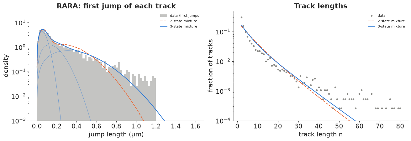
Left (log scale): the three-state mixture follows the first-jump distribution through its peak, its shoulder at 0.1-0.3 µm (which the two-state model misses) and most of its tail; beyond about 0.9 µm the data are heavier than either model, and they end at the tracker's 1.2 µm search radius. Three fixed $D$'s are a coarse description of what may be a continuum of mobilities: letting each state's $D$ vary between molecules (a log-normal spread per state, integrated out on a quadrature grid) gave a posterior with r_hat 1.5-2.4 in a prototype - the states overlap and trade places - which is the motivation for the non-parametric "state arrays" of saSPT. Right: the geometric track-length laws capture lengths from 3 to about 35 positions. The data have more two-position tracks than predicted (30% against 17%; short fragments from blinking or mis-linking) and a heavier tail of very long tracks, i.e. survival is not quite constant.
The out-of-focus bias
What would we conclude from the "good" tracks only? A common practice is to keep tracks with at least 10 positions and ignore how long tracks are. We refit the 3-state model that way and compare the state fractions.
long_idx = np.flatnonzero(lens_rara >= 10)
mix_long = fit(mixture_model([rara_tracks[i] for i in long_idx], lens_rara[long_idx], 3, use_length=False),
               "RARA, 3 states, tracks >= 10 positions, no length term")
frac = pd.DataFrame({
    "all tracks + length model": post_mean(mix[3], "w"),
    "tracks >= 10 positions only": post_mean(mix_long, "w"),
    "D (all tracks)": post_mean(mix[3], "D"),
    "D (long tracks)": post_mean(mix_long, "D")},
    index=["bound", "slow", "fast"])
print(frac.round(3).to_string())
q3 = post_mean(mix[3], "q")
print("mean number of displacements per track, by state:", np.round(1 / (1 - q3), 1))
RARA, 3 states, tracks >= 10 positions, no length term: 5 s, divergences 0, max r_hat 1.002, min ESS 974
       all tracks + length model  tracks >= 10 positions only  D (all tracks)  D (long tracks)
bound                      0.375                        0.480           0.023            0.021
slow                       0.257                        0.270           0.916            0.733
fast                       0.367                        0.249           6.327            4.753
mean number of displacements per track, by state: [9.7 7.6 3.9]
Keeping only tracks with at least 10 positions raises the bound fraction from 38% to 48% and cuts the fast fraction from 37% to 25%; the fast state's $D$ also drops from 6.3 to 4.8 µm²/s, because the fastest molecules are the first to leave the focal slice. The survival probabilities explain why: a bound molecule gives on average 9.7 displacements before it is lost, a fast one 3.9. Any selection on track length is a selection on the state. Modelling the loss (here a per-state geometric law; in Spot-On a calculated escape probability from a slice of known depth) lets all tracks count. The weights are still fractions of tracks, not of molecules in the nucleus: a free molecule also enters the focal slice more often than a bound one. Converting one into the other needs a model of the axial motion, which is what Spot-On's defocalisation correction does.
A hierarchy across cells: the free control
The HaloTag-NLS control comes from eleven nuclei, some with a few hundred tracks, some with a thousand. Cells differ (nuclear crowding, expression level, focus), so each nucleus $c$ gets its own free-state $D_c$ and bound fraction $f_c$, partially pooled: $\log D_c \sim \mathcal N(\mu_D, \tau_D)$, $\operatorname{logit} f_c \sim \mathcal N(\mu_f, \tau_f)$ (non-centred), with a shared $\sigma$, a shared immobile-state $D_0$ and per-state survival. Two states suffice for a control: anything "bound" here is an immobile artefact or a non-specific interaction, and its fraction should be small.
nls_cells = np.unique(nls_region)
cell_idx = pd.Index(nls_cells).get_indexer(nls_region)
lens_nls = lengths["nls"]
z2n, ccn, idxn = pack_tracks(nls_tracks, CAP)
with pm.Model(coords={"cell": nls_cells, "state": ["immobile", "free"]}) as nls_model:
    logD0 = pm.Normal("logD_immobile", np.log(0.03), 1.5)
    mu_D = pm.Normal("mu_logD_free", np.log(5.0), 1.0)
    tau_D = pm.HalfNormal("tau_logD", 0.3)
    logD_c = pm.Deterministic("logD_free", mu_D + tau_D * pm.Normal("zD", 0, 1, dims="cell"), dims="cell")
    mu_f = pm.Normal("mu_logit_f", -2.0, 1.5)
    tau_f = pm.HalfNormal("tau_logit_f", 1.0)
    f_c = pm.Deterministic("f_immobile", pm.math.sigmoid(mu_f + tau_f * pm.Normal("zf", 0, 1, dims="cell")), dims="cell")
    sigma_n = pm.LogNormal("sigma", np.log(0.03), 0.5)
    q_n = pm.Beta("q", 2.0, 2.0, dims="state")
    pm.Deterministic("D_free", pt.exp(logD_c), dims="cell")
    pm.Deterministic("D_free_pop", pt.exp(mu_D))
    D_trk = pt.stack([pt.exp(logD0) + 0 * logD_c[cell_idx], pt.exp(logD_c[cell_idx])], axis=1)   # tracks x 2
    v = 2 * D_trk[idxn] * DT + 2 * sigma_n**2 * (1 - ccn)[:, None]
    lpm = -pt.log(2 * np.pi * v) - z2n[:, None] / (2 * v)
    lpt = pt.inc_subtensor(pt.zeros((len(nls_tracks), 2))[idxn], lpm)
    lpt = lpt + pt.log1p(-q_n)[None] + (lens_nls[:, None] - 2) * pt.log(q_n)[None]
    logw = pt.stack([pt.log(f_c[cell_idx]), pt.log1p(-f_c[cell_idx])], axis=1)
    pm.Potential("lik", pt.logsumexp(logw + lpt, axis=1).sum())
idata_nls = fit(nls_model, "NLS, 2 states, 11 cells", target_accept=0.9,
                var_names=["logD_immobile", "mu_logD_free", "tau_logD", "mu_logit_f", "tau_logit_f", "sigma",
                           "q", "D_free", "D_free_pop", "f_immobile", "logD_free"])
print(az.summary(idata_nls, var_names=["D_free_pop", "tau_logD", "tau_logit_f", "sigma", "q"], round_to=3).iloc[:, :4].to_string())
print(f"immobile D: {np.exp(post_mean(idata_nls, 'logD_immobile')):.3f} µm²/s")
NLS, 2 states, 11 cells: 34 s, divergences 0, max r_hat 1.004, min ESS 391
               mean     sd  eti89_lb  eti89_ub
D_free_pop   10.216  0.694     9.125    11.336
tau_logD      0.208  0.056     0.139     0.308
tau_logit_f   0.575  0.157     0.373     0.860
sigma         0.045  0.001     0.044     0.047
q[immobile]   0.871  0.005     0.863     0.879
q[free]       0.700  0.003     0.695     0.705
immobile D: 0.143 µm²/sfig, axes = plt.subplots(1, 2, figsize=(13, 4.4))
n_cell = np.bincount(cell_idx)
order = np.argsort(n_cell)
Dc = idata_nls.posterior["D_free"]
fc = idata_nls.posterior["f_immobile"]
ax = axes[0]
for pos, c in enumerate(order):
q_ = np.quantile(Dc.isel(cell=c).values, [0.055, 0.5, 0.945])
ax.plot([q_[0], q_[2]], [pos, pos], color=BLUE, lw=2)
ax.plot(q_[1], pos, "o", color=BLUE, ms=5)
pop = np.quantile(idata_nls.posterior["D_free_pop"].values, [0.055, 0.945])
ax.axvspan(*pop, color=AQUA, alpha=0.2, label="population median, 89%")
ax.set_yticks(range(len(order)), [f"cell {nls_cells[c]} ({n_cell[c]} tracks)" for c in order])
ax.set(xlabel="free D (µm²/s)", title="HaloTag-NLS: free D per nucleus")
ax.legend(fontsize=8)
ax = axes[1]
for pos, c in enumerate(order):
q_ = np.quantile(fc.isel(cell=c).values, [0.055, 0.5, 0.945])
ax.plot([q_[0], q_[2]], [pos, pos], color=PURPLE, lw=2)
ax.plot(q_[1], pos, "o", color=PURPLE, ms=5)
rara_bound = mix[3].posterior["w"].isel(state=0).values.ravel()
ax.axvspan(*np.quantile(rara_bound, [0.055, 0.945]), color=BLUE, alpha=0.2, label="RARA bound fraction (3 states)")
ax.set_yticks(range(len(order)), [""] * len(order))
ax.set(xlabel="immobile fraction (at first jump)", title="Immobile fraction", xlim=(0, None))
ax.legend(fontsize=8);
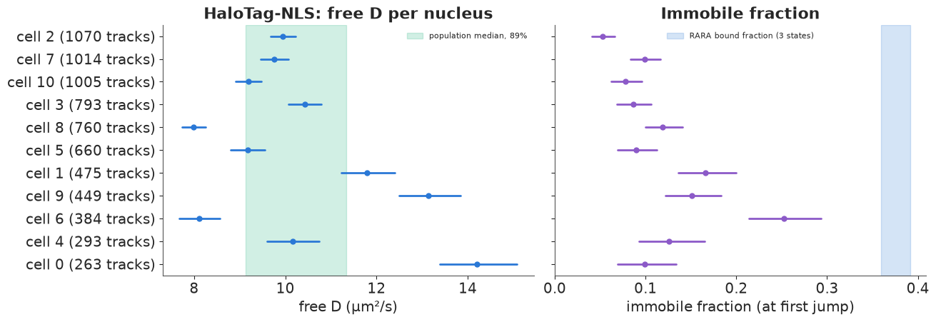
The control behaves as a control should: the free state dominates, with a population median $D$ of about 10 µm²/s (89%: 9.1-11.3) - faster than RARA's fast state, as expected for the smaller, non-binding HaloTag-NLS - and a small immobile fraction (5-25% by nucleus, against 38% bound for RARA). The immobile state's $D$ is 0.14 µm²/s, six times RARA's bound state: whatever it is (aggregates, nuclear-envelope sticking, mis-linked tracks), it is not chromatin binding. The hierarchy has little to shrink - every nucleus has hundreds of tracks - but it answers a different question: between-nucleus variation is real and large. The sd of $\log D$ between nuclei is about 0.2 (89%: 0.14-0.31), so free $D$ ranges from 8 to 14 µm²/s across cells while each cell's own interval is only ±3-6%. Pooling all tracks as if from one cell would report a $D$ ten times more precise than the next experiment can reproduce. (The control's effective $\sigma$, 45 nm, is again above its reported 34 nm.)
6 · Switching inside a track: a hidden Markov model that knows about localisation error
The mixture gives every track one state. But molecules bind and unbind during a track: a jump of a free molecule, a few frames of stillness, another jump. A hidden Markov model (E24) lets the state $s_k$ of each displacement follow a Markov chain with transition matrix $\Gamma$, and the forward algorithm sums over all $K^{n}$ state paths.
E24's forward algorithm needs emissions that are independent given the states. Here they are not: $\Delta_k$ and $\Delta_{k+1}$ share the error $e_{k+1}$. Tools such as vbSPT (Persson et al. 2013) ignore this and use $\Delta_k \mid s_k \sim \mathcal N(0, 2D_{s_k}\Delta t + 2\sigma^2)$. We will see what that costs. The exact alternative writes the track as a switching linear-Gaussian model in the current error: $\Delta_k = w_k + e_{k+1} - e_k$, $w_k \sim \mathcal N(0, 2D_{s_k}\Delta t)$, $e_k \sim \mathcal N(0, \sigma^2)$. For a fixed state path a Kalman filter on $e$ is exact; summed over paths, the filter's Gaussian becomes a mixture with $K^k$ components. The standard remedy is GPB1 (generalised pseudo-Bayes; Bar-Shalom & Li): carry, for each current state $i$, the forward probability $\alpha_k(i)$ and one Gaussian $\mathcal N(m_i, P_i)$ for the current error; at every step,
- for each previous state $j$ and new state $i$: predict $\Delta_k \sim \mathcal N(-m_j,\, 2D_i\Delta t + \sigma^2 + P_j)$ , score it, and update the error $e_{k+1} \mid \Delta_k$ is Gaussian with gain ($\sigma^2 / V_{ij}$);
- $\alpha_{k+1}(i) = \sum_j \alpha_k(j)\,\Gamma_{ji}\,\text{score}_{ij}$ (the usual forward step);
- collapse the $K$ Gaussians arriving in state $i$ into one by moment matching.
With one state this is the Kalman filter, so it is exact (checked below against the
sine-basis likelihood); with several it is an approximation that is excellent when states
persist for several frames. It runs in a pytensor.scan over time, vectorised over tracks
(padded, with a mask that freezes a finished track), with the transition matrix, $D$'s and
$\sigma$ passed as non_sequences (closing over model variables inside a scan fails at
gradient time).
def gpb_forward_np(d, mask, D, sigma, logG, logpi, dt=DT):
    """NumPy GPB1 forward filter. d: (T, N, 2) displacements, mask (T, N).
    Returns per-track log-likelihood and filtered state probabilities (T, N, K)."""
    T, N, _ = d.shape
    K, s2 = len(D), sigma**2
    la = np.broadcast_to(logpi, (N, K)).copy()
    m, P = np.zeros((N, K, 2)), np.full((N, K), s2)
    filt = np.zeros((T, N, K))
    for k in range(T):
        V = 2 * D[None, None, :] * dt + s2 + P[:, :, None]                 # N x prev j x new i
        r = d[k][:, None, None, :] + m[:, :, None, :]
        a = la[:, :, None] + logG[None] - np.log(2 * np.pi * V) - (r**2).sum(-1) / (2 * V)
        la_new = logsumexp(a, axis=1)
        wgt = np.exp(a - la_new[:, None, :])
        mij, Pij = (s2 / V)[..., None] * r, s2 - s2**2 / V
        m_new = (wgt[..., None] * mij).sum(1)
        P_new = (wgt * (Pij + ((mij - m_new[:, None]) ** 2).mean(-1))).sum(1)
        ok = mask[k][:, None]
        la, m, P = np.where(ok, la_new, la), np.where(ok[..., None], m_new, m), np.where(ok, P_new, P)
        filt[k] = np.exp(la - logsumexp(la, axis=1, keepdims=True))
    return logsumexp(la, axis=1), filt


def gpb_loglik_pt(d, mask, D, sigma, logG, logpi):
    """The same filter in PyTensor (scan over time, vectorised over tracks)."""
    s2 = sigma**2
    N, K = d.shape[1], D.shape[0]

    def step(dk, ok, la, m, P, D, s2, logG):
        V = 2 * D[None, None, :] * DT + s2 + P[:, :, None]
        r = dk[:, None, None, :] + m[:, :, None, :]
        a = la[:, :, None] + logG[None] - pt.log(2 * np.pi * V) - (r**2).sum(-1) / (2 * V)
        la_new = pt.logsumexp(a, axis=1)
        wgt = pt.exp(a - la_new[:, None, :])
        mij, Pij = (s2 / V)[..., None] * r, s2 - s2**2 / V
        m_new = (wgt[..., None] * mij).sum(1)
        P_new = (wgt * (Pij + ((mij - m_new[:, None]) ** 2).mean(-1))).sum(1)
        return (pt.switch(ok[:, None], la_new, la), pt.switch(ok[:, None, None], m_new, m),
                pt.switch(ok[:, None], P_new, P))

    la, _, _ = pytensor.scan(
        step, sequences=[pt.as_tensor(d), pt.as_tensor(mask.astype("int8"))],
        outputs_info=[pt.zeros((N, K)) + logpi[None], pt.zeros((N, K, 2)), pt.zeros((N, K)) + s2],
        non_sequences=[D, s2, logG], return_updates=False)
    return pt.logsumexp(la[-1], axis=1)


def indep_loglik_pt(d, mask, D, sigma, G, pi):
    """Textbook HMM: displacements independent given the state, variance 2 D dt + 2 sigma^2."""
    var = 2 * D * DT + 2 * sigma**2
    lE = -pt.log(2 * np.pi * var)[None, None] - (d**2).sum(-1)[..., None] / (2 * var)[None, None]

    def step(le, ok, la, G):
        return pt.switch(ok[:, None], pt.logsumexp(la[:, :, None] + pt.log(G)[None], axis=1) + le, la)

    la = pytensor.scan(step, sequences=[lE[1:], pt.as_tensor(mask[1:].astype("int8"))],
                       outputs_info=[pt.log(pi)[None] + lE[0]], non_sequences=[G], return_updates=False)
    return pt.logsumexp(la[-1], axis=1)


# exactness check with one state against the sine basis
t_chk = simulate_track(25, 0.2, 0.03, rng, exposure=0.03)
d_chk = np.diff(t_chk, axis=0)
Qc, cc_chk = dst_basis(len(d_chk))
exact = stats.norm(0, np.sqrt(mode_var(0.2, 0.03, cc_chk))[:, None]).logpdf(Qc @ d_chk).sum()
gpb1 = gpb_forward_np(d_chk[:, None], np.ones((len(d_chk), 1), bool), np.array([0.2]), 0.03,
                      np.zeros((1, 1)), np.zeros(1))[0][0]
print(f"one state: sine-basis {exact:.10f}, GPB1 filter {gpb1:.10f}")
one state: sine-basis 61.8326771915, GPB1 filter 61.8326771915
Does it work? A simulation with known switching
100 tracks of 40 positions switch between bound ($D = 0.03$) and free ($D = 3$ µm²/s) with a 5% chance per frame of leaving either state (a mean stay of 20 frames, 0.15 s), $\sigma = 35$ nm. We fit both HMMs with the same priors: ordered $\log D$ as before, $\sigma$ as before, and a sticky Dirichlet(21, 1) row for each state's transition probabilities (prior mean 95% stay).
def hmm_model(d, mask, K=2, exact=True):
    mu0 = [np.log(0.03), np.log(3.0)] if K == 2 else [np.log(0.02), np.log(0.8), np.log(5.0)]
    with pm.Model(coords={"state": np.arange(K), "to": np.arange(K)}) as model:
        logD = pm.Normal("logD", mu0, 1.5, dims="state", transform=pm.distributions.transforms.ordered)
        sigma = pm.LogNormal("sigma", np.log(0.03), 0.5)
        G = pm.Dirichlet("Gamma", a=np.eye(K) * 20 + 1, dims=("state", "to"))
        D = pm.Deterministic("D", pt.exp(logD), dims="state")
        A = pt.concatenate([(pt.eye(K) - G).T, pt.ones((1, K))], axis=0)     # stationary distribution
        pi = pt.linalg.solve(A.T @ A, A.T @ np.r_[np.zeros(K), 1.0])
        ll = gpb_loglik_pt(d, mask, D, sigma, pt.log(G), pt.log(pi)) if exact else indep_loglik_pt(d, mask, D, sigma, G, pi)
        pm.Potential("lik", ll.sum())
    return model


def simulate_switching(n, D, sigma, Gamma, rng):
    pi = np.linalg.lstsq(np.vstack([(np.eye(len(D)) - Gamma).T, np.ones(len(D))]), np.r_[np.zeros(len(D)), 1], rcond=None)[0]
    s = np.zeros(n - 1, int)
    s[0] = rng.choice(len(D), p=pi)
    for k in range(1, n - 1):
        s[k] = rng.choice(len(D), p=Gamma[s[k - 1]])
    steps = rng.normal(0, 1, (n - 1, 2)) * np.sqrt(2 * D[s] * DT)[:, None]
    return np.vstack([np.zeros(2), np.cumsum(steps, 0)]) + rng.normal(0, sigma, (n, 2)), s


rng6 = np.random.default_rng(6)
D_sw, sig_sw, G_sw = np.array([0.03, 3.0]), 0.035, np.array([[0.95, 0.05], [0.05, 0.95]])
sw = [simulate_switching(40, D_sw, sig_sw, G_sw, rng6) for _ in range(100)]
d_sw = np.stack([np.diff(x, axis=0) for x, _ in sw], axis=1)
mask_sw = np.ones(d_sw.shape[:2], bool)
s_sw = np.stack([s for _, s in sw], axis=1)
hmm_sim = {}
for exact, lab in [(True, "GPB1 (error-aware)"), (False, "independent emissions")]:
    hmm_sim[lab] = fit(hmm_model(d_sw, mask_sw, exact=exact), f"simulated switching, {lab}", compile_kwargs=JAX)
    print(az.summary(hmm_sim[lab], var_names=["D", "sigma"], round_to=4).iloc[:, :4].to_string())
simulated switching, GPB1 (error-aware): 17 s, divergences 0, max r_hat 1.004, min ESS 836
         mean      sd  eti89_lb  eti89_ub
D[0]   0.0345  0.0026    0.0305    0.0389
D[1]   3.1060  0.0756    2.9851    3.2277
sigma  0.0346  0.0007    0.0336    0.0357
simulated switching, independent emissions: 33 s, divergences 0, max r_hat 1.013, min ESS 285
mean sd eti89_lb eti89_ub
D[0] 0.0585 0.0511 0.0039 0.1551
D[1] 3.1303 0.0920 2.9861 3.2812
sigma 0.0310 0.0070 0.0171 0.0378The two fits agree on the free state and on the transition probabilities, but not on the bound state:
- The error-aware GPB1 model recovers $\sigma$ = 34.6 nm (89%: 33.6-35.7; truth 35) and bound $D$ = 0.035 µm²/s (0.031-0.039; truth 0.03, just below the interval - a small bias from the moment-matching collapse or chance). It sampled in about 10 s with the JAX backend.
- The textbook HMM, which ignores the correlation, can only learn $2D\Delta t + 2\sigma^2$ for the bound state: bound $D$ spans 0.004-0.16 µm²/s (a factor of 40) and $\sigma$ 17-38 nm. The information that separates them is the negative correlation between successive displacements, which that model throws away. Its r_hat (1.013) and ESS (285) show the ridge too.
Both classify the steps equally well (98% correct): which state a step is in shows in the jump size, not in the correlations. So the independent-emission HMM is fine for segmenting tracks and poor for measuring the bound state's mobility - and it is the bound state's mobility that reveals chromatin dynamics (section 7).
Which state, when? Smoothed state probabilities
The forward pass gives $p(s_k \mid \Delta_{1:k})$. For $p(s_k \mid \text{whole track})$ we combine it with the same filter run backwards in time (the model is time-reversible when the chain starts in its stationary distribution): $p(s_k \mid \text{all}) \propto p(s_k \mid \Delta_{1:k})\, p(s_k \mid \Delta_{k+1:n}) / \pi(s_k)$ - the two-filter smoother, approximate here because past and future also share the error $e_{k+1}$. We average it over 40 posterior draws.
def smoothed_probs(idata, d, mask, n_draws=40):
    post = az.extract(idata, var_names=["D", "sigma", "Gamma"], num_samples=n_draws, random_seed=RANDOM_SEED)
    out = 0.0
    for i in range(n_draws):
        D_ = post["D"].values[:, i]
        s_ = float(post["sigma"].values[i])
        G_ = post["Gamma"].values[..., i]
        K = len(D_)
        pi_ = np.linalg.lstsq(np.vstack([(np.eye(K) - G_).T, np.ones(K)]), np.r_[np.zeros(K), 1], rcond=None)[0]
        _, fw = gpb_forward_np(d, mask, D_, s_, np.log(G_), np.log(pi_))
        # backward: reverse each track within its own length so that padding stays at the end
        n_i = mask.sum(0)
        d_rev = np.zeros_like(d)
        for j, nn in enumerate(n_i):
            d_rev[:nn, j] = d[:nn, j][::-1]
        G_rev = G_.T * pi_[None, :] / pi_[:, None]                      # P(s_k = j | s_k+1 = i)
        _, bw_rev = gpb_forward_np(d_rev, mask, D_, s_, np.log(G_rev), np.log(pi_))
        bw = np.broadcast_to(pi_, fw.shape).copy()                     # padding: prior (unused)
        for j, nn in enumerate(n_i):
            b = bw_rev[:nn, j][::-1]                                     # p(s_k | d_k..d_n)
            bw[:nn, j] = np.vstack([b[1:] @ G_rev, pi_[None]])            # p(s_k | d_k+1..d_n)
        sm = fw * bw / pi_
        out = out + sm / sm.sum(-1, keepdims=True) / n_draws
    return out


p_sw = smoothed_probs(hmm_sim["GPB1 (error-aware)"], d_sw, mask_sw)
p_sw_ind = smoothed_probs(hmm_sim["independent emissions"], d_sw, mask_sw)
print(f"state accuracy (P(free) > 0.5): GPB1 {np.mean((p_sw[..., 1] > 0.5) == s_sw):.3f}, "
      f"independent {np.mean((p_sw_ind[..., 1] > 0.5) == s_sw):.3f}")

fig, axes = plt.subplots(1, 3, figsize=(15, 4.4))
ax = axes[0]
for lab, col in [("GPB1 (error-aware)", BLUE), ("independent emissions", ORANGE)]:
    ax.plot(hmm_sim[lab].posterior["D"].isel(state=0).values.ravel(),
            hmm_sim[lab].posterior["sigma"].values.ravel() * 1e3, ".", ms=1.5, alpha=0.3, color=col, label=lab)
ax.plot(D_sw[0], sig_sw * 1e3, "*", ms=14, color=INK, label="truth")
ax.set(xscale="log", xlabel="bound D (µm²/s)", ylabel="σ (nm)", title="Bound state: D against σ")
ax.legend(handles=[plt.Line2D([], [], ls="", marker="o", color=BLUE, label="GPB1 (error-aware)"),
                   plt.Line2D([], [], ls="", marker="o", color=ORANGE, label="independent emissions"),
                   plt.Line2D([], [], ls="", marker="*", ms=10, color=INK, label="truth")], fontsize=8)
ax = axes[1]
j = int(np.argmax([np.abs(np.diff(s)).sum() for s in s_sw.T]))
k_ax = np.arange(d_sw.shape[0])
ax.fill_between(k_ax, 0, s_sw[:, j], step="mid", color=GREY, alpha=0.3, label="true state (free = 1)")
ax.plot(k_ax, p_sw[:, j, 1], "-o", ms=3, color=BLUE, label="P(free), GPB1")
ax.set(xlabel="frame", ylabel="P(free)", title="One simulated track")
ax.legend(fontsize=8)
ax = axes[2]
x_j = sw[j][0]
sc = ax.scatter(x_j[1:, 0], x_j[1:, 1], c=p_sw[:, j, 1], cmap="coolwarm", vmin=0, vmax=1, s=18, zorder=3)
ax.plot(x_j[:, 0], x_j[:, 1], color=GREY, lw=0.6)
fig.colorbar(sc, ax=ax, label="P(free)")
ax.set(xlabel="x (µm)", ylabel="y (µm)", title="The same track in the plane")
ax.set_aspect("equal", adjustable="datalim");
state accuracy (P(free) > 0.5): GPB1 0.977, independent 0.976
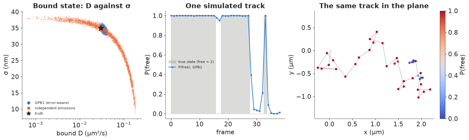
Left: the posterior draws of bound $D$ and $\sigma$: the independent-emission model's (orange) lie along the curve $2D\Delta t + 2\sigma^2 = $ const, the GPB1 draws (blue) form a small cluster on the truth. Middle and right: the smoothed probability of the free state follows the true path of one simulated track, switching within one or two frames of each true switch; a two-frame bound visit near frame 16 is only hinted at (P(free) dips to 0.95), and a one-frame free visit near frame 33 is picked up.
The RARA tracks
We fit the two-state GPB1 model to the 320 RARA tracks with at least 20 positions (first 61 positions of each: up to 60 displacements, 10,897 in all).
MIN_HMM, CAP_HMM = 20, 61
hmm_tracks = [t[:CAP_HMM] for t in rara_tracks if len(t) >= MIN_HMM]
hmm_err = [e[:CAP_HMM] for e in rara_err if len(e) >= MIN_HMM]
T_h = CAP_HMM - 1
d_h = np.zeros((T_h, len(hmm_tracks), 2))
mask_h = np.zeros((T_h, len(hmm_tracks)), bool)
for i, t in enumerate(hmm_tracks):
    dd = np.diff(t, axis=0)
    d_h[: len(dd), i], mask_h[: len(dd), i] = dd, True
print(f"{len(hmm_tracks)} tracks, {mask_h.sum()} displacements")
hmm_rara = fit(hmm_model(d_h, mask_h), "RARA, 2-state GPB1 HMM", compile_kwargs=JAX)
print(az.summary(hmm_rara, var_names=["D", "sigma", "Gamma"], round_to=4).iloc[:, :4].to_string())
G_post = hmm_rara.posterior["Gamma"]
dwell_ms = DT * 1e3 / (1 - G_post.sel(state=0, to=0).values.ravel())
dwell_free_ms = DT * 1e3 / (1 - G_post.sel(state=1, to=1).values.ravel())
print(f"mean stay in the bound state: {np.median(dwell_ms):.0f} ms "
      f"(89%: {np.quantile(dwell_ms, 0.055):.0f}-{np.quantile(dwell_ms, 0.945):.0f}); "
      f"free: {np.median(dwell_free_ms):.0f} ms")
320 tracks, 10897 displacements
RARA, 2-state GPB1 HMM: 54 s, divergences 0, max r_hat 1.001, min ESS 1379
               mean      sd  eti89_lb  eti89_ub
D[0]         0.0222  0.0009    0.0208    0.0236
D[1]         2.7650  0.0639    2.6636    2.8699
sigma        0.0325  0.0003    0.0320    0.0329
Gamma[0, 0]  0.9811  0.0016    0.9785    0.9835
Gamma[0, 1]  0.0189  0.0016    0.0165    0.0215
Gamma[1, 0]  0.0567  0.0052    0.0487    0.0650
Gamma[1, 1]  0.9433  0.0052    0.9350    0.9513
mean stay in the bound state: 396 ms (89%: 347-453); free: 132 ms
p_h = smoothed_probs(hmm_rara, d_h, mask_h)
n_h = mask_h.sum(0)
n_switch = np.array([np.abs(np.diff(p_h[: n_h[i], i, 1] > 0.5)).sum() for i in range(len(hmm_tracks))])
always_bound = np.array([np.all(p_h[: n_h[i], i, 0] > 0.9) for i in range(len(hmm_tracks))])
print(f"tracks with at least one switch: {np.mean(n_switch > 0):.0%}; "
f"bound (P > 0.9) at every step: {np.mean(always_bound):.0%}")
fig, axes = plt.subplots(1, 3, figsize=(15, 4.6))
show = np.flatnonzero(n_switch > 0)[:3]
for ax, i in zip(axes, show):
t = hmm_tracks[i]
sc = ax.scatter(t[1:, 0], t[1:, 1], c=p_h[: n_h[i], i, 1], cmap="coolwarm", vmin=0, vmax=1, s=16, zorder=3)
ax.plot(t[:, 0], t[:, 1], color=GREY, lw=0.6)
ax.set(xlabel="x (µm)", ylabel="y (µm)", title=f"RARA track {i}: {n_h[i]} displacements")
ax.set_aspect("equal", adjustable="datalim")
fig.colorbar(sc, ax=axes, label="P(free)", shrink=0.8);
tracks with at least one switch: 39%; bound (P > 0.9) at every step: 43%
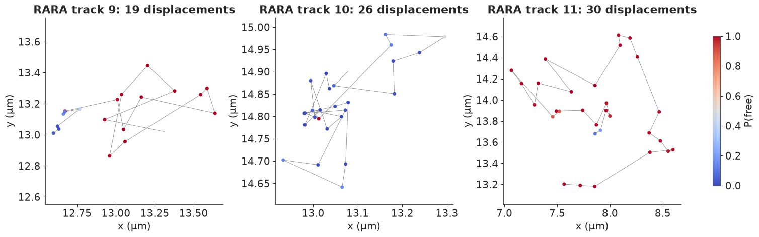
The HMM finds a bound state at 0.022 µm²/s and a free one at 2.8 µm²/s (the long tracks carry few fast molecules, so "free" here mostly means the slow state of section 5). A bound molecule leaves the bound state with probability 1.9% per frame: a mean stay of about 400 ms (89%: 350-450 ms) while in view; the free state lasts about 130 ms. Because the forward algorithm simply stops at the end of a track, bleaching and defocusing censor these dwell times without biasing them - under the model's assumption that losing a molecule does not depend on how long it has been bound. Stays of chromatin-bound transcription factors are often seconds long when measured with slow imaging designed for that purpose (long exposures blur free molecules away); a 7.48 ms movie of short tracks sees mainly the short, transient interactions. 39% of the long tracks switch at least once, and 43% are confidently bound (P > 0.9) at every step. The three tracks above show typical switches: a molecule that unbinds and leaves (track 9), a bound molecule with a few large jumps that the model is unsure about (track 10), and a free molecule that pauses briefly (track 11). A three-state HMM is the natural next step; with the same code it took about four minutes to sample in a prototype, beyond this notebook's budget (exercise 2).
Note the effective error again: $\sigma$ = 32.5 nm, against a reported 16 nm for the localisations in these long tracks (printed below). The HMM's bound state is Brownian; if the bound molecules' displacements anticorrelate more than Brownian motion plus error allows, the model can only absorb that with a larger $\sigma$. Section 7 tests exactly this.
7 · Is it anomalous? Fractional Brownian motion and fake subdiffusion
A bound transcription factor moves with its piece of chromatin, and chromatin is a polymer: its loci are known to move subdiffusively, $\text{MSD} \propto \tau^\alpha$ with $\alpha < 1$. The simplest Gaussian model with that property is fractional Brownian motion (fBM) with Hurst exponent $H = \alpha/2$: per coordinate $\langle (x(t) - x(s))^2 \rangle = 2K|t-s|^\alpha$, and the displacements are stationary with the Toeplitz covariance
$$\operatorname{Cov}(\Delta_k, \Delta_{k+l}) = K\Delta t^\alpha\big(|l+1|^\alpha - 2|l|^\alpha + |l-1|^\alpha\big) + \sigma^2 (2\,[l = 0] - [|l| = 1]).$$
For $\alpha < 1$ successive displacements anticorrelate at every lag (the molecule is pulled back), for $\alpha > 1$ they correlate (superdiffusion), $\alpha = 1$ is Brownian. Localisation error adds a lag-1 anticorrelation - which is exactly what a little subdiffusion looks like over short tracks. This is the question of the AnDi challenge (Muñoz-Gil et al. 2021, on simulated benchmark tracks): is this motion anomalous, and what is $\alpha$?
This covariance is no longer tridiagonal, so no fixed basis diagonalises it: we use a batched Cholesky factor, one 30 × 30 matrix per track. Each track $i$ has its own $\alpha_i = 2\,\text{logit}^{-1}(\mu_\alpha + \tau_\alpha z_i)$ (partial pooling, $\alpha \in (0, 2)$) and its own amplitude, which we parameterise by the MSD at lag 6 frames, $2K(6\Delta t)^\alpha$, not by $K$: $K$ and $\alpha$ trade off strongly (a change in $\alpha$ rotates the MSD line about $\tau = 1$ s, far outside the data), and the lag-6 amplitude decorrelates them (this cut the sampling time by 2-3x in a prototype).
Priors: $\mu_\alpha \sim \mathcal N(0, 1)$ (so $\alpha_{\text{pop}}$ is centred on 1), $\tau_\alpha \sim$ HalfNormal(0.5); the amplitudes are pooled too, log $\text{MSD}_6 \sim \mathcal N(\mu_m, \tau_m)$ with $\mu_m \sim \mathcal N(\log(12 \cdot 0.03\,\Delta t), 1.5)$ and $\tau_m \sim$ HalfNormal(1) (why, below); $\sigma$ as before. First the trap, on 30 simulated Brownian tracks ($D = 0.02$ µm²/s, $\sigma = 30$ nm, 31 positions): fit fBM without and with the error term.
M_F = 30
LAG = np.abs(np.subtract.outer(np.arange(M_F), np.arange(M_F))).astype(float)
# log|l+1|, log|l|, log|l-1| with log 0 floored: x**a = exp(a log x) then has a finite gradient
# in a at x = 0 (0**a differentiates to 0 * log 0 = NaN)
LOGS = [np.log(np.maximum(np.abs(LAG + k), 1e-300)) for k in (1, 0, -1)]
LREF = 6


def fbm_model(d, with_error=True, sigma_prior=(np.log(0.03), 0.5)):
    """d: (tracks, M_F, 2) displacements."""
    N = d.shape[0]
    with pm.Model(coords={"track": np.arange(N)}) as model:
        mu_a = pm.Normal("mu_alpha", 0.0, 1.0)
        tau_a = pm.HalfNormal("tau_alpha", 0.5)
        alpha = pm.Deterministic("alpha", 2 * pm.math.sigmoid(mu_a + tau_a * pm.Normal("z", 0, 1, dims="track")), dims="track")
        pm.Deterministic("alpha_pop", 2 * pm.math.sigmoid(mu_a))
        mu_m = pm.Normal("mu_log_msd6", np.log(2 * 0.03 * LREF * DT), 1.5)
        tau_m = pm.HalfNormal("tau_log_msd6", 1.0)
        log_msd6 = pm.Deterministic("log_msd6", mu_m + tau_m * pm.Normal("z_m", 0, 1, dims="track"), dims="track")
        K = pt.exp(log_msd6 - np.log(2) - alpha * np.log(LREF * DT))
        s2 = pm.LogNormal("sigma", *sigma_prior) ** 2 if with_error else 0.0
        a = alpha[:, None, None]
        C = K[:, None, None] * DT**a * (pt.exp(a * LOGS[0]) - 2 * pt.exp(a * LOGS[1]) + pt.exp(a * LOGS[2]))
        C = C + s2 * (2 * (LAG == 0) - (LAG == 1))[None] + 1e-10 * np.eye(M_F)[None]
        L = pt.linalg.cholesky(C)
        zz = pt.linalg.solve_triangular(L, d, lower=True, b_ndim=2)                # (N, M_F, 2)
        logdet = pt.log(pt.diagonal(L, axis1=1, axis2=2)).sum()
        pm.Potential("lik", -0.5 * (zz**2).sum() - 2 * logdet - N * M_F * np.log(2 * np.pi))
    return model


rng7 = np.random.default_rng(7)
x_bm = np.cumsum(rng7.normal(0, np.sqrt(2 * 0.02 * DT), (30, M_F + 1, 2)), axis=1) + rng7.normal(0, 0.03, (30, M_F + 1, 2))
d_bm = np.diff(x_bm, axis=1)
fbm_sim = {}
for we, lab in [(False, "fBM, no error term"), (True, "fBM + localisation error")]:
    fbm_sim[lab] = fit(fbm_model(d_bm, we), f"Brownian simulation, {lab}", compile_kwargs=JAX, draws=500)
    print(az.summary(fbm_sim[lab], var_names=["alpha_pop", "tau_alpha"] + (["sigma"] if we else []),
                     round_to=3).iloc[:, :4].to_string())
Brownian simulation, fBM, no error term: 15 s, divergences 0, max r_hat 1.007, min ESS 336
            mean     sd  eti89_lb  eti89_ub
alpha_pop  0.369  0.024     0.330     0.409
tau_alpha  0.155  0.092     0.023     0.310
Brownian simulation, fBM + localisation error: 15 s, divergences 0, max r_hat 1.007, min ESS 740
mean sd eti89_lb eti89_ub
alpha_pop 1.050 0.111 0.865 1.225
tau_alpha 0.234 0.174 0.021 0.554
sigma 0.030 0.001 0.028 0.031The trap works as advertised. Ignoring the error, the population exponent of these Brownian tracks is 0.37 (89%: 0.33-0.41): confident, strong, and entirely fake subdiffusion. The error's lag-1 anticorrelation is read as a molecule being pulled back. With the error term, $\alpha_{\text{pop}}$ = 1.05 (0.87-1.23), consistent with the truth, and $\sigma$ is recovered (30 nm).
A modelling note that cost a prototype: with an independent amplitude per track (log MSD$_6$ with a fixed prior instead of the hierarchy used here), the same kind of simulated Brownian data gave $\alpha_{\text{pop}}$ near 1.1 in four of five datasets, some with 89% intervals excluding 1. With only 30 displacements per track, a free nuisance parameter per track biases the shared shape parameter (a Neyman-Scott-type problem). Pooling the amplitudes removed it (medians 0.87-0.97 on three of the same datasets).
Bound RARA molecules
Now the real question. We take the RARA tracks with at least 31 positions that the HMM of section 6 calls bound ($P > 0.9$) at every one of their first 30 steps - long stretches of a molecule sitting on chromatin.
bound_idx = [i for i, t in enumerate(hmm_tracks)
             if len(t) > M_F and np.all(p_h[:M_F, i, 0] > 0.9)]
d_bound = np.array([np.diff(hmm_tracks[i][: M_F + 1], axis=0) for i in bound_idx])
err_rms = np.sqrt(np.mean(np.concatenate([hmm_err[i][: M_F + 1] for i in bound_idx]) ** 2))
print(f"{len(d_bound)} bound tracks with {M_F} displacements; "
      f"rms of the reported localisation errors: {err_rms * 1e3:.1f} nm")
fbm_real = {}
for we, sp, lab in [(False, None, "fBM, no error term"),
                    (True, (np.log(0.03), 0.5), "fBM + localisation error"),
                    (True, (np.log(err_rms), 0.1), "fBM + error, σ prior from the reported errors")]:
    fbm_real[lab] = fit(fbm_model(d_bound, we, sp), f"RARA bound, {lab}", compile_kwargs=JAX, draws=500)
    print(az.summary(fbm_real[lab], var_names=["alpha_pop", "tau_alpha"] + (["sigma"] if we else []),
                     round_to=3).iloc[:, :4].to_string())
a_tr = fbm_real["fBM + error, σ prior from the reported errors"].posterior["alpha"]
p_sub = (a_tr < 1).mean(("chain", "draw")).values
print(f"tracks with P(alpha < 1) > 0.9: {np.mean(p_sub > 0.9):.0%}; with P(alpha > 1) > 0.9: {np.mean(p_sub < 0.1):.0%}")
84 bound tracks with 30 displacements; rms of the reported localisation errors: 16.3 nm
RARA bound, fBM, no error term: 49 s, divergences 0, max r_hat 1.010, min ESS 567
            mean     sd  eti89_lb  eti89_ub
alpha_pop  0.316  0.019     0.286     0.346
tau_alpha  0.403  0.075     0.286     0.525
RARA bound, fBM + localisation error: 35 s, divergences 0, max r_hat 1.010, min ESS 567
mean sd eti89_lb eti89_ub
alpha_pop 0.372 0.031 0.324 0.423
tau_alpha 0.456 0.085 0.324 0.599
sigma 0.012 0.002 0.009 0.015RARA bound, fBM + error, σ prior from the reported errors: 35 s, divergences 0, max r_hat 1.008, min ESS 756
mean sd eti89_lb eti89_ub
alpha_pop 0.398 0.030 0.353 0.446
tau_alpha 0.491 0.089 0.352 0.640
sigma 0.015 0.001 0.013 0.016
tracks with P(alpha < 1) > 0.9: 100%; with P(alpha > 1) > 0.9: 0%fig, axes = plt.subplots(1, 3, figsize=(15, 4.4))
ax = axes[0]
for src, lab, col, ls, idt in [
("simulated Brownian", "fBM, no error term", ORANGE, "--", fbm_sim["fBM, no error term"]),
("simulated Brownian", "fBM + error", BLUE, "--", fbm_sim["fBM + localisation error"]),
("RARA bound", "fBM, no error term", ORANGE, "-", fbm_real["fBM, no error term"]),
("RARA bound", "fBM + error", BLUE, "-", fbm_real["fBM + localisation error"]),
("RARA bound", "fBM + error, reported σ", AQUA, "-", fbm_real["fBM + error, σ prior from the reported errors"])]:
v = idt.posterior["alpha_pop"].values.ravel()
ax.hist(v, bins=64, range=(0, 1.6), density=True, histtype="step", lw=1.5, ls=ls, color=col, label=f"{src}: {lab}")
ax.axvline(1, color=INK, lw=0.8)
ax.set(xlabel="population α", ylabel="density", title="Anomalous exponent α = 2H")
ax.legend(fontsize=7, loc="upper left")
ax = axes[1]
med = a_tr.median(("chain", "draw")).values
qlo, qhi = a_tr.quantile([0.055, 0.945], dim=("chain", "draw")).values
o = np.argsort(med)
ax.vlines(np.arange(len(o)), qlo[o], qhi[o], color=BLUE, lw=1)
ax.plot(np.arange(len(o)), med[o], "o", ms=3, color=BLUE)
ax.axhline(1, color=INK, lw=0.8)
ax.set(xlabel="bound track (sorted)", ylabel="α (89% interval)", title="Per-track α (σ prior from reported errors)")
ax = axes[2]
lg = np.arange(1, 16)
xb = np.cumsum(np.concatenate([np.zeros((len(d_bound), 1, 2)), d_bound], axis=1), axis=1)
emp_msd = np.array([np.mean(np.sum((xb[:, k:] - xb[:, :-k]) ** 2, axis=2)) for k in lg])
ax.plot(lg * DT, emp_msd, "o", color=INK, ms=4, label="data (ensemble)")
post = az.extract(fbm_real["fBM + error, σ prior from the reported errors"], var_names=["alpha", "log_msd6", "sigma"], num_samples=300,
random_seed=RANDOM_SEED)
al, lm, sg = post["alpha"].values, post["log_msd6"].values, post["sigma"].values
curves = np.array([np.mean(2 * 2 * np.exp(lm[:, s])[:, None] / 2 * (lg[None] / LREF) ** al[:, s][:, None], axis=0)
+ 4 * sg[s] ** 2 for s in range(al.shape[1])])
ax.fill_between(lg * DT, *np.quantile(curves, [0.055, 0.945], axis=0), color=BLUE, alpha=0.3, label="fBM + error (reported σ), 89%")
bm_line = emp_msd[0] + (lg - 1) * (emp_msd[1] - emp_msd[0])
ax.plot(lg * DT, bm_line, "--", color=GREY, label="Brownian: MSD linear in τ through lags 1-2")
ax.set(xscale="log", yscale="log", xlabel="lag τ (s)", ylabel="MSD (µm²)", title="Bound RARA: ensemble MSD")
ax.legend(fontsize=8);
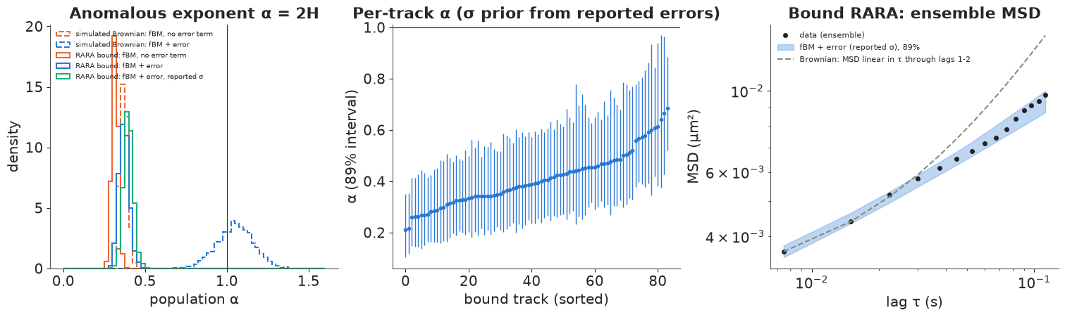
Left: on the Brownian simulation (dashed) the error term moves $\alpha$ from a false 0.37 to the truth. On the bound RARA tracks (solid, 84 tracks) it moves much less: from 0.32 without the error to 0.37 (89%: 0.32-0.42) with a free $\sigma$, and 0.40 (0.35-0.45) when $\sigma$ gets an informative prior from the reported localisation errors (rms 16 nm; posterior 15 nm). This subdiffusion survives the correction: bound RARA molecules move subdiffusively with $\alpha \approx 0.4$ - consistent with the range reported for chromatin loci in mammalian nuclei. Note that the free-$\sigma$ fit puts $\sigma$ at 12 nm, below the reported errors: $\sigma$ and $\alpha$ still trade off, and the independent calibration of the error is what pins them down. Middle: every one of the 84 tracks has $P(\alpha < 1) > 0.9$, with medians from 0.2 to 0.7 (the between-track sd on the logit scale is about 0.5): chromatin mobility is heterogeneous. Right: the ensemble MSD of these tracks bends below the Brownian line through its first two points; by 110 ms the Brownian extrapolation overshoots the data by about 60%, and the fBM posterior follows the bend.
This also explains the effective errors of sections 5 and 6: a Brownian bound state needs $\sigma$ = 32-38 nm to mimic the extra anticorrelation of subdiffusion, twice the reported error. The caveats: the tracks were selected as bound by a Brownian HMM, which favours tracks with small, confined motion; 30 displacements (0.22 s) cannot distinguish fBM from other subdiffusive models (confinement in a small domain, continuous-time random walks) - the AnDi challenge's other question; and motion blur, which we could not quantify for these movies, would add a positive lag-1 correlation and slightly raise $\alpha$.
Summary
| question | model | answer here |
|---|---|---|
| what is a track's likelihood? | Gaussian displacements, tridiagonal (MA(1)) covariance from localisation error and blur; exact and scan-free in the sine eigenbasis | checked against the dense MvNormal to 10 decimals |
| $D$ of one short track? | per-track $D$, $\sigma$ | MSD(1) overestimates bound $D$ threefold; a 4-point MSD line is negative for 13% of tracks; the likelihood is near unbiased with 91% coverage of 89% intervals |
| how many states, what fractions? | mixture over whole tracks with per-state survival | RARA: bound 0.023, slow 0.9, fast 6.3 µm²/s; 38/26/37% of tracks; 3 states beat 2 by ~2,450 elpd |
| what does selecting long tracks do? | same mixture, long tracks only | bound fraction 38% → 48%, fast 37% → 25% |
| cell-to-cell variation? | hierarchy over 11 control nuclei | free $D$ ≈ 10 µm²/s, between-cell sd ≈ 20% |
| binding and unbinding inside tracks? | HMM with a GPB1 filter that carries the error | bound stay ≈ 0.4 s in view; the textbook HMM cannot separate bound $D$ from $\sigma$ |
| is bound motion anomalous? | fBM with error, hierarchical α | α ≈ 0.4; without the error term Brownian tracks look like α ≈ 0.37 |
- Localisation error is the main character. It inflates naive $D$, makes MSD fits noisy, hides the bound state's mobility from textbook HMMs and fakes subdiffusion. The fix each time is the same: put the error in the likelihood, where it shows as a negative lag-1 correlation.
- Short tracks and the frame rate set what is identifiable: a track gives $2D\Delta t + 2\sigma^2$ easily and the split only with length; blur and error are not separable from tracks at all. Independent information (reported localisation errors) is worth using as a prior.
- What you keep decides what you find: fast molecules leave focus first, so a state's fraction depends on how track loss is handled; the tracker's search radius truncates the fastest jumps.
- Effective parameters flag misspecification: a fitted $\sigma$ twice the reported one was the first sign that bound RARA is not Brownian.
Try it yourself
- Motion blur. Simulate full-frame exposure ($R = 1/6$) for a free molecule at $D = 5$
µm²/s with $\sigma = 30$ nm, and fit it with $R = 0$. Show that the fitted $\sigma$ collapses (it
estimates $\sigma^2 - 2DR\Delta t$, which is negative here) and that $D$ is biased; then fit with the
correct $R$ in
mode_var. What happens if you give $R$ its own prior? - A three-state HMM. Fit
hmm_model(d_h, mask_h, K=3)(about four minutes). Does the slow state of section 5 appear inside tracks, and do molecules pass through it on the way to binding (compare $\Gamma_{\text{fast} \to \text{bound}}$ with $\Gamma_{\text{fast} \to \text{slow}}$)? - Confinement instead of fBM. Replace fBM by an Ornstein-Uhlenbeck (harmonically confined) position, $x_{k+1} = \phi x_k + \eta_k$ with $\phi = e^{-\kappa\Delta t}$, observed with error - a Kalman filter or its stationary Toeplitz covariance $\operatorname{Cov}(x_k, x_{k+l}) = \frac{D}{\kappa}\phi^{|l|}$ per coordinate. Compare it with fBM on the bound RARA tracks by per-track LOO (compute the per-track log-likelihoods from the Cholesky factors). Which kind of subdiffusion do the data prefer?