Choosing between things
A lot of applied statistics is about choices among a small set of alternatives: which supplier, which travel mode, which product on a shelf, which contract. The standard tool is the discrete choice model (McFadden, Nobel prize 2000), and its workhorse is the logit. It is used to price products, forecast demand for things that do not exist yet, value time and environmental goods, and plan transport networks.
The data here are a classic stated-preference (conjoint) experiment run by Kenneth Train for US electricity suppliers in the late 1990s, when retail electricity markets were being opened to competition. Each respondent saw up to 12 screens like this one and picked one supplier:
| supplier 1 | supplier 2 | supplier 3 | supplier 4 | |
|---|---|---|---|---|
| price | 7 c/kWh fixed | 9 c/kWh fixed | time-of-day rates | seasonal rates |
| contract length | 5 years | 1 year | none | 5 years |
| local company | no | yes | no | no |
| well-known company | yes | no | no | yes |
Because the attributes are varied by design, the choices tell us how people trade them off: how many cents per kWh is a local supplier worth? How much does a 5-year lock-in cost? And because every person answers 12 times, we can see how much people differ.
The question we end with is a business one: a new, unknown, non-local supplier enters this market. What price and contract should it offer, and whose customers will it take?
The plan
- The data and the random-utility model
- The conditional logit: priors, fit, a check against maximum likelihood
- What the logit gets wrong: IIA and a person-level predictive check
- The mixed logit: random coefficients, LKJ, and the price-coefficient trap
- Willingness to pay: population, heterogeneity, individuals
- Model comparison: what does "leave one out" mean for panel choice data?
- A known-truth check (simulated)
- Substitution patterns and a market simulator: the pricing decision
import logging
import time
import warnings

import arviz as az
import matplotlib.pyplot as plt
import numpy as np
import pandas as pd
import pymc as pm
import pytensor
import pytensor.tensor as pt
import xarray as xr
from scipy import optimize, special, stats

from pymc_challenges import data

RANDOM_SEED = 68
rng = np.random.default_rng(RANDOM_SEED)
az.style.use("arviz-variat")
logging.getLogger("pymc").setLevel(logging.WARNING)  # several fits: no sampler banner each
warnings.filterwarnings("ignore", category=RuntimeWarning, module="arviz")  # NaN r_hat of constants
warnings.filterwarnings("ignore", message="Estimated shape parameter of Pareto")  # we print k-hat counts
BLUE, ORANGE, AQUA, GREY, PURPLE, RED = "#2a78d6", "#eb6834", "#1baf7a", "#8a8a86", "#8c5ac8", "#c8384e"
print(f"PyMC {pm.__version__}, ArviZ {az.__version__}, PyTensor {pytensor.__version__}")


def q(x, probs=(0.05, 0.5, 0.95), axis=None):
    """Posterior quantiles, rounded for printing."""
    return np.round(np.quantile(x, probs, axis=axis), 2)
PyMC 6.3.2, ArviZ 1.3.0, PyTensor 3.3.2
data.describe("electricity_choice")
raw = data.load("electricity_choice").sort_values(["chid", "alt"]).reset_index(drop=True)
raw.head(8)
electricity_choice: Stated-preference choice experiment: 361 residential customers each made up to 12 choices (4,308 choice tasks; 348 people did all 12) among 4 hypothetical electricity suppliers. Long format, one row per task x alternative (17,232 rows): choice (1 if chosen), id (person), alt (1-4, unlabelled), pf (fixed price, cents/kWh: 7 or 9; 0 when the contract is time-of-day or seasonal), cl (contract length in years: 0, 1 or 5; switching early costs a penalty), loc (local company), wk (well-known company), tod (time-of-day rates: 11c 8am-8pm, 5c otherwise), seas (seasonal rates: 10c summer, 8c winter, 6c spring/fall), chid (choice-task id).
  source: Kenneth Train's stated-preference survey of electricity suppliers (Huber & Train 2001, Marketing Letters 12:259-269; Revelt & Train 2000, UC Berkeley working paper), distributed as `Electricity` in the R package mlogit (GPL >= 2) and, in long format, in the Python package xlogit (GPL-3; the URL). Verified identical, value for value, to mlogit 2.0-0's data/Electricity.rda.
  url:    https://raw.githubusercontent.com/arteagac/xlogit/master/examples/data/electricity_long.csv
| choice | id | alt | pf | cl | loc | wk | tod | seas | chid | |
|---|---|---|---|---|---|---|---|---|---|---|
| 0 | 0 | 1 | 1 | 7 | 5 | 0 | 1 | 0 | 0 | 1 |
| 1 | 0 | 1 | 2 | 9 | 1 | 1 | 0 | 0 | 0 | 1 |
| 2 | 0 | 1 | 3 | 0 | 0 | 0 | 0 | 0 | 1 | 1 |
| 3 | 1 | 1 | 4 | 0 | 5 | 0 | 1 | 1 | 0 | 1 |
| 4 | 0 | 1 | 1 | 7 | 0 | 0 | 1 | 0 | 0 | 2 |
| 5 | 0 | 1 | 2 | 9 | 5 | 0 | 1 | 0 | 0 | 2 |
| 6 | 1 | 1 | 3 | 0 | 1 | 1 | 0 | 1 | 0 | 2 |
| 7 | 0 | 1 | 4 | 0 | 5 | 0 | 0 | 0 | 1 | 2 |
Choice data come in long format: each choice task contributes one row per alternative, and a 0/1 column marks the chosen one. For modelling we reshape to a 3-D array $X_{t j a}$ (task $t$, alternative $j$, attribute $a$) and a vector of chosen alternatives $y_t$.
One recoding matters. A time-of-day (TOD) or seasonal contract has no fixed price (pf is 0),
so in the raw coding the TOD dummy absorbs the whole price of a TOD contract and its
coefficient is large (about -5.5, see below). Both variable-rate schedules average 8 c/kWh
(TOD: 11c for 12 day hours and 5c for 12 night hours; seasonal: 10/8/6 c, averaging 8c if use is
flat over the year), so we give those contracts a price of 8 and keep the dummy. The dummy then
means the extra dislike of a variable-rate contract beyond its average price. For fixed
coefficients this is an exact reparameterisation (the likelihood is the same), and it puts every
coefficient on a scale of about 1, which helps priors and interpretation.
T, J = raw.chid.nunique(), 4
ATTR = ["price", "contract", "local", "known", "tod", "seas"]
LABEL = {"price": "price (c/kWh)", "contract": "contract length (yr)", "local": "local company",
         "known": "well-known company", "tod": "time-of-day rates", "seas": "seasonal rates"}


def as_grid(col):
    return raw[col].to_numpy(float).reshape(T, J)


variable = (as_grid("tod") + as_grid("seas")) > 0
X = np.stack([np.where(variable, 8.0, as_grid("pf")), as_grid("cl"), as_grid("loc"),
              as_grid("wk"), as_grid("tod"), as_grid("seas")], axis=-1)   # (task, alt, attr)
y = as_grid("choice").argmax(axis=1)                                     # chosen alternative
people, pid = np.unique(raw["id"].to_numpy().reshape(T, J)[:, 0], return_inverse=True)
N = len(people)
tasks_per = np.bincount(pid)
print(f"{N} people, {T} choice tasks, {J} alternatives each; tasks per person: "
      f"{dict(zip(*np.unique(tasks_per, return_counts=True)))}")
print("attribute levels:", {a: np.unique(X[..., k]).tolist() for k, a in enumerate(ATTR)})
print(f"every task offers at least one variable-rate contract: {variable.any(axis=1).all()}; "
      f"a local supplier is offered in {X[..., 2].max(axis=1).mean():.0%} of tasks")
361 people, 4308 choice tasks, 4 alternatives each; tasks per person: {np.int64(8): np.int64(2), np.int64(9): np.int64(2), np.int64(10): np.int64(1), np.int64(11): np.int64(8), np.int64(12): np.int64(348)}
attribute levels: {'price': [7.0, 8.0, 9.0], 'contract': [0.0, 1.0, 5.0], 'local': [0.0, 1.0], 'known': [0.0, 1.0], 'tod': [0.0, 1.0], 'seas': [0.0, 1.0]}
every task offers at least one variable-rate contract: True; a local supplier is offered in 79% of tasks1.2 · What people chose
Before any model: how often is an alternative chosen, by attribute level? With four alternatives, 25% is the "no preference" line.
chosen = np.zeros((T, J), bool)
chosen[np.arange(T), y] = True
isvar_chosen = variable[np.arange(T), y]
var_count = np.bincount(pid, weights=isvar_chosen, minlength=N)   # variable-rate picks per person
loc_offered = X[..., 2].max(axis=1) > 0
loc_chosen = X[np.arange(T), y, 2] > 0

fig, axes = plt.subplots(1, 3, figsize=(15, 4), width_ratios=[1.6, 1, 1])
groups = [("price", [7, 8, 9], "{:g}c"), ("contract", [0, 1, 5], "{:g} yr"),
          ("local", [0, 1], None), ("known", [0, 1], None), ("tod", [1], None), ("seas", [1], None)]
xpos, ticks, labels, cols = 0, [], [], []
for k, (a, levels, fmt) in enumerate(groups):
    idx = ATTR.index(a)
    for lev in levels:
        m = X[..., idx] == lev
        if a == "price" and lev == 8:
            m &= ~variable            # no fixed-price contract costs 8c
            if not m.any():
                continue
        rate = chosen[m].mean()
        axes[0].bar(xpos, rate, color=[BLUE, ORANGE, AQUA, PURPLE, RED, GREY][k], width=0.8)
        ticks.append(xpos)
        labels.append(fmt.format(lev) if fmt else f"{a}\n" + ("yes" if lev else "no"))
        xpos += 1
    xpos += 0.6
axes[0].axhline(0.25, color="k", lw=1, ls="--")
axes[0].set_xticks(ticks, labels, fontsize=8)
axes[0].set(ylabel="share of offers chosen", title="Choice rate by attribute level")
axes[1].hist(var_count[tasks_per == 12], bins=np.arange(14) - 0.5, color=RED)
axes[1].set(xlabel="variable-rate contracts chosen (of 12)", ylabel="people",
            title="Some never choose TOD/seasonal")
share_loc = pd.Series(loc_chosen[loc_offered]).groupby(pid[loc_offered]).mean()
axes[2].hist(share_loc, bins=np.linspace(0, 1, 13), color=AQUA)
axes[2].set(xlabel="share of offers with a local supplier\nin which one was chosen", ylabel="people",
            title="...and some always go local");
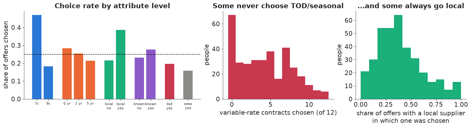
The marginal patterns are strong and sensible: cheap beats expensive, short contracts beat long ones, local and well-known companies are popular, variable-rate contracts are unpopular. The right two panels show something the averages hide: people are very different. Among the 348 people who did all 12 tasks, a large group never picked a time-of-day or seasonal contract, although every single task offered one, and at the other end some chose one most of the time. Local suppliers split people the same way. Keep this picture in mind; the first model will not be able to reproduce it.
1.3 · Random utility
Person $i$ in task $t$ gets utility from alternative $j$
$$U_{itj} = \underbrace{\beta^\top x_{tj}}_{V_{tj}} + \varepsilon_{itj},$$
a systematic part that depends on the attributes and a part the analyst does not see. The person picks the alternative with the largest utility. If the $\varepsilon$ are independent Gumbel (type-I extreme value) with scale 1, the probability that $j$ has the largest utility has a closed form (McFadden 1974):
$$P(y_t = j) = \frac{\exp V_{tj}}{\sum_k \exp V_{tk}} = \operatorname{softmax}(V_t)_j .$$
Two consequences follow directly:
- Only differences in utility matter. Adding a constant to every $V_{tj}$ changes nothing, so there is no intercept (the alternatives here are unlabelled; with labelled alternatives - bus, car, train - you would add $J - 1$ alternative-specific constants).
- Only ratios of coefficients have units. The standard deviation of $\varepsilon$ is fixed at $\pi/\sqrt 6$, so $\beta$ is measured in units of unobserved noise. A coefficient's size is not interpretable on its own, but $-\beta_{\text{local}} / \beta_{\text{price}}$ is: it is the price increase (c/kWh) that exactly offsets having a local supplier - the willingness to pay (WTP).
2 · The conditional logit
2.1 · Priors, checked on the choice scale
What does "a vague prior" mean for a choice model? Draw coefficients, compute the choice probabilities on the real design, and look at the probability of the most likely alternative in each task. Near 0.25 means coin flips; near 1 means deterministic choices.
def max_prob(beta):
    """beta: (draws, attr) -> max choice probability per draw and task."""
    return special.softmax(np.einsum("tja,sa->stj", X, beta), axis=2).max(axis=2)


prior_sds = {"Normal(0, 10)": 10.0, "Normal(0, 2)": 2.0}
fig, ax = plt.subplots(figsize=(8, 3.4))
for (name, s), col in zip(prior_sds.items(), [GREY, BLUE]):
    b = np.random.default_rng(1).normal(0, s, size=(300, 6))
    mp = max_prob(b).ravel()
    ax.hist(mp, bins=np.linspace(0.25, 1, 61), density=True, histtype="step", lw=2, color=col,
            label=f"{name}: {np.mean(mp > 0.99):.0%} of tasks have P(max) > 0.99")
ax.set(xlabel="probability of the most likely alternative (prior predictive, real design)",
       ylabel="density", title="A 'vague' prior claims people choose deterministically")
ax.legend(fontsize=8);
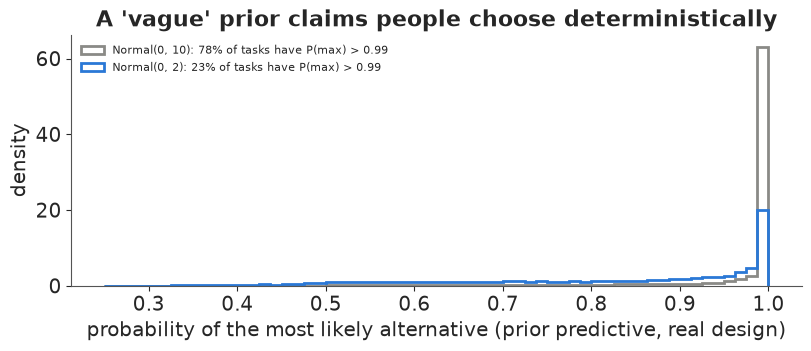
Normal(0, 10) on the coefficients is not vague about choices at all: it says that in most tasks one alternative is chosen with near certainty, because a price coefficient of -10 per cent makes a 2-cent difference worth 20 units of noise. Normal(0, 2) still allows strong preferences (tasks with $P > 0.99$ are common) but also plenty of real uncertainty. We use it for the logit. Attributes are in natural units (cents, years, 0/1), all of order 1-10, so one scale is acceptable here.
2.2 · The model in PyMC
The long data become a (task, alt, attr) array; utility is a dot product over attr;
pm.Categorical(logit_p=...) applies the softmax over alt.
coords = {"task": np.arange(T), "alt": [1, 2, 3, 4], "attr": ATTR, "person": people}
with pm.Model(coords=coords) as m_logit:
    Xd = pm.Data("X", X, dims=("task", "alt", "attr"))
    beta = pm.Normal("beta", 0, 2, dims="attr")
    V = (Xd * beta).sum(axis=-1)                        # (task, alt) utilities
    pm.Categorical("y", logit_p=V, observed=y, dims="task")

t0 = time.time()
with m_logit:
    idata_logit = pm.sample(random_seed=RANDOM_SEED)
    pm.compute_log_likelihood(idata_logit)
    pm.sample_posterior_predictive(idata_logit, extend_inferencedata=True, random_seed=RANDOM_SEED)
print(f"sampled in {time.time() - t0:.0f} s, tuning steps "
      f"{idata_logit.posterior.attrs.get('tuning_steps')}, "
      f"divergences {int(idata_logit.sample_stats['diverging'].sum())}")
az.summary(idata_logit, var_names=["beta"], round_to=3)
sampled in 6 s, tuning steps 400, divergences 0
| mean | sd | eti89_lb | eti89_ub | ess_bulk | ess_tail | r_hat | mcse_mean | mcse_sd | |
|---|---|---|---|---|---|---|---|---|---|
| beta[price] | -0.626 | 0.023 | -0.663 | -0.590 | 3376.511 | 3360.940 | 1.002 | 0.000 | 0.000 |
| beta[contract] | -0.108 | 0.008 | -0.122 | -0.095 | 3938.191 | 3403.167 | 1.002 | 0.000 | 0.000 |
| beta[local] | 1.442 | 0.050 | 1.361 | 1.523 | 2473.392 | 2403.430 | 1.000 | 0.001 | 0.001 |
| beta[known] | 0.996 | 0.045 | 0.925 | 1.068 | 2420.351 | 2934.311 | 1.001 | 0.001 | 0.001 |
| beta[tod] | -0.461 | 0.043 | -0.529 | -0.392 | 3672.199 | 3264.066 | 1.001 | 0.001 | 0.001 |
| beta[seas] | -0.838 | 0.046 | -0.912 | -0.766 | 3492.804 | 3209.416 | 1.002 | 0.001 | 0.001 |
A check against maximum likelihood. The logit log-likelihood is concave, so a 6-parameter optimiser finds the MLE immediately. With 4,308 tasks the posterior mean should sit on it. We also fit the original coding (TOD/seasonal price absorbed by the dummies) to confirm the recoding is only a reparameterisation.
def logit_nll(b, XX):
    v = XX @ b
    return -(v[np.arange(T), y] - special.logsumexp(v, axis=1)).sum()


X_orig = X.copy()
X_orig[..., 0] = as_grid("pf")
mle = optimize.minimize(logit_nll, np.zeros(6), args=(X,), method="BFGS")
mle_orig = optimize.minimize(logit_nll, np.zeros(6), args=(X_orig,), method="BFGS")
post_mean = idata_logit.posterior["beta"].mean(("chain", "draw")).to_numpy()
print(pd.DataFrame({"posterior mean": post_mean, "MLE": mle.x, "MLE, original coding": mle_orig.x},
                   index=ATTR).round(3))
print(f"max log-likelihood: {-mle.fun:.2f} (recoded) vs {-mle_orig.fun:.2f} (original)")
print(f"implied original-coding TOD coefficient: tod + 8 * price = {mle.x[4] + 8 * mle.x[0]:.3f}")
          posterior mean    MLE  MLE, original coding
price             -0.626 -0.625                -0.625
contract          -0.108 -0.108                -0.108
local              1.442  1.442                 1.442
known              0.996  0.996                 0.996
tod               -0.461 -0.461                -5.463
seas              -0.838 -0.838                -5.840
max log-likelihood: -4958.65 (recoded) vs -4958.65 (original)
implied original-coding TOD coefficient: tod + 8 * price = -5.463
Identical log-likelihoods, the TOD and seasonal coefficients map exactly ($-0.461 + 8 \times (-0.625) = -5.463$), and the posterior means agree with the MLE to the second decimal. With this much data and a concave likelihood the prior hardly matters for the logit; it will matter more once each person gets their own coefficients.
The logit says: one cent per kWh costs 0.63 utility units; a local supplier is worth $1.44 / 0.63 \approx 2.3$ c/kWh, a well-known one 1.6 c/kWh, each year of contract -0.17 c/kWh, and a variable-rate contract is worth less than a fixed contract at the same average price (0.7 c/kWh less for TOD, 1.3 c/kWh for seasonal). Before believing these numbers, check the model.
3 · What the logit gets wrong
3.1 · IIA: independence of irrelevant alternatives
The logit implies that the ratio of any two choice probabilities, $P_j / P_k = \exp(V_j - V_k)$, does not depend on what else is on offer. A consequence is that a new alternative takes customers from all existing ones in proportion to their shares, no matter how similar it is to each. The textbook case (Debreu 1960's "red bus / blue bus"): if half of commuters take the car and half the red bus, adding a blue bus identical to the red one should leave the car's share at 1/2, but the logit predicts 1/3. We will measure this on the fitted models in section 8.
IIA holds for one person with fixed tastes. It fails for a population of people with different tastes: the new blue bus draws its riders from people who liked buses, not from car lovers. So the deeper problem with the logit is the one visible in section 1.2: it gives everyone the same $\beta$.
3.2 · A person-level posterior predictive check
The logit reproduces aggregate choice shares well - it is fitted to them. The panel structure gives a much sharper test: replicate all 12 answers of every person and count, for each person, how many variable-rate contracts they chose. If everybody shares one $\beta$, the counts are a sum of independent Bernoulli trials and cannot pile up at 0.
def person_counts(yrep):
    """yrep: (draws, task) replicated choices -> (draws, person) variable-rate picks."""
    picks = variable[np.arange(T)[None, :], yrep]
    return np.stack([np.bincount(pid, weights=p, minlength=N) for p in picks])


def count_hist(counts, full=tasks_per == 12):
    c = counts[..., full] if counts.ndim == 2 else counts[full]
    return np.stack([(c == k).sum(axis=-1) for k in range(13)], axis=-1)


def yrep_draws(idata, n=400):
    yr = idata.posterior_predictive["y"].stack(s=("chain", "draw")).transpose("s", "task")
    return yr.to_numpy()[:: yr.shape[0] // n][:n].astype(int)


obs_hist = count_hist(var_count)
rep_logit = count_hist(person_counts(yrep_draws(idata_logit)))
never_logit = rep_logit[:, 0]
print(f"people (of 348 with 12 tasks) who never chose a variable-rate contract: observed "
      f"{obs_hist[0]}, logit replications 5-50-95%: {q(never_logit)}")
people (of 348 with 12 tasks) who never chose a variable-rate contract: observed 67, logit replications 5-50-95%: [0. 1.5 4. ]
The logit expects one or two such people (at most 4 in 90% of replications); there are 67. This is not a small misfit: the model cannot represent people who consistently avoid something. The fix is to let each person have their own coefficients.
4 · The mixed logit
4.1 · Random coefficients
Give person $i$ their own coefficient vector, drawn from a population distribution:
$$\beta_i \sim \mathcal N(\mu, \Sigma), \qquad P(y_{it} = j \mid \beta_i) = \operatorname{softmax}(X_t \beta_i)_j .$$
This is the mixed logit (random-parameters logit; Revelt & Train 1998, McFadden & Train 2000). Conditional on $\beta_i$ it is a logit, so IIA holds for each person, but the population choice probability $\int \operatorname{softmax}(X_t\beta)\,\mathcal N(\beta\mid\mu,\Sigma)\,d\beta$ no longer has IIA. McFadden and Train showed it can approximate any random-utility model. The panel matters: because the same $\beta_i$ enters all 12 of a person's answers, repeated choices identify how people differ, not only how they choose on average.
In PyMC, $\Sigma$ gets an LKJ prior on its correlation matrix plus half-normal scales, and the person effects are non-centred: $\beta_i = \mu + L z_i$ with $z_i \sim \mathcal N(0, I)$ and $L$ the Cholesky factor. With 12 binary-ish answers per person, each person's data are weak, which is where non-centred parameterisations work best.
4.2 · First attempt: everything normal
The obvious specification makes all six coefficients normal, including price.
def mixed_logit(lognormal_price, X_=X, y_=y, pid_=pid, n_people=N):
    c = coords | {"task": np.arange(len(y_)), "person": np.arange(n_people)}
    with pm.Model(coords=c) as m:
        Xd = pm.Data("X", X_, dims=("task", "alt", "attr"))
        # for the lognormal price, mu[price] is the mean of log(-beta_price)
        mu = pm.Normal("mu", [-0.5 if lognormal_price else 0.0, 0, 0, 0, 0, 0],
                       [1.0 if lognormal_price else 2.0, 2, 2, 2, 2, 2], dims="attr")
        chol, _, _ = pm.LKJCholeskyCov("chol", n=6, eta=2.0, compute_corr=True,
                                       sd_dist=pm.HalfNormal.dist(2.0, shape=6))
        z = pm.Normal("z", 0, 1, dims=("person", "attr"))
        raw_b = mu + z @ chol.T                               # non-centred N(mu, L L^T)
        if lognormal_price:
            raw_b = pt.concatenate([-pt.exp(raw_b[:, :1]), raw_b[:, 1:]], axis=1)
        b = pm.Deterministic("beta", raw_b, dims=("person", "attr"))
        V = (Xd * b[pid_][:, None, :]).sum(axis=-1)
        pm.Categorical("y", logit_p=V, observed=y_, dims="task")
    return m


def fit(model, seed=RANDOM_SEED):
    t0 = time.time()
    with model:
        idata = pm.sample(random_seed=seed)
    print(f"sampled in {time.time() - t0:.0f} s; divergences "
          f"{int(idata.sample_stats['diverging'].sum())}; max tree depth "
          f"{int(idata.sample_stats['depth'].max())}; r_hat max (mu, chol, z) "
          f"{max(float(az.rhat(idata.posterior[v]).max()) for v in ['mu', 'chol', 'z']):.3f}; "
          f"bulk ESS min (mu, chol) "
          f"{min(float(az.ess(idata.posterior[v]).min()) for v in ['mu', 'chol']):.0f}")
    return idata


m_normal = mixed_logit(lognormal_price=False)
idata_normal = fit(m_normal)
az.summary(idata_normal, var_names=["mu", "chol_stds"], round_to=3)
sampled in 18 s; divergences 0; max tree depth 5; r_hat max (mu, chol, z) 1.020; bulk ESS min (mu, chol) 286
| mean | sd | eti89_lb | eti89_ub | ess_bulk | ess_tail | r_hat | mcse_mean | mcse_sd | |
|---|---|---|---|---|---|---|---|---|---|
| mu[price] | -1.102 | 0.068 | -1.212 | -0.996 | 1455.257 | 1767.295 | 1.001 | 0.002 | 0.001 |
| mu[contract] | -0.264 | 0.030 | -0.313 | -0.219 | 1342.912 | 2082.021 | 1.004 | 0.001 | 0.000 |
| mu[local] | 2.639 | 0.167 | 2.373 | 2.911 | 1097.630 | 1552.530 | 1.003 | 0.005 | 0.003 |
| mu[known] | 1.989 | 0.127 | 1.783 | 2.191 | 1213.221 | 1851.030 | 1.002 | 0.004 | 0.002 |
| mu[tod] | -1.570 | 0.208 | -1.908 | -1.246 | 808.569 | 1674.331 | 1.002 | 0.007 | 0.004 |
| mu[seas] | -1.702 | 0.163 | -1.963 | -1.440 | 1387.857 | 2019.166 | 1.002 | 0.004 | 0.002 |
| chol_stds[0] | 0.903 | 0.072 | 0.790 | 1.022 | 1322.027 | 1885.265 | 1.001 | 0.002 | 0.001 |
| chol_stds[1] | 0.454 | 0.029 | 0.410 | 0.503 | 1264.447 | 1988.497 | 1.002 | 0.001 | 0.000 |
| chol_stds[2] | 2.283 | 0.163 | 2.030 | 2.545 | 1038.852 | 1595.062 | 1.000 | 0.005 | 0.003 |
| chol_stds[3] | 1.640 | 0.131 | 1.439 | 1.857 | 1025.002 | 1531.845 | 1.001 | 0.004 | 0.002 |
| chol_stds[4] | 3.256 | 0.214 | 2.923 | 3.610 | 907.559 | 1386.472 | 1.002 | 0.007 | 0.004 |
| chol_stds[5] | 2.405 | 0.162 | 2.151 | 2.669 | 1092.128 | 1729.677 | 1.001 | 0.005 | 0.003 |
The sampler is happy. The model, looked at as a description of people, is not: with a mean price coefficient near -1.1 and a standard deviation near 0.9, the population distribution puts a sizeable share of people on a positive price coefficient - customers who prefer to pay more. That is not plausible for electricity at the same service quality, and it poisons the one quantity we most want: willingness to pay, which divides by the price coefficient.
tri = np.tril_indices(6)


def hyper(idata, S, seed=0):
    """S posterior draws of mu (S, 6) and the Cholesky factor L (S, 6, 6)."""
    post = az.extract(idata, var_names=["mu", "chol"], num_samples=S, random_seed=seed)
    L = np.zeros((S, 6, 6))
    L[:, tri[0], tri[1]] = post["chol"].transpose("sample", ...).to_numpy()
    return post["mu"].transpose("sample", ...).to_numpy(), L


def population(idata, lognormal_price, S=1000, R=500, seed=1):
    """Coefficients of R simulated people for each of S posterior draws: (S, R, 6)."""
    mu, L = hyper(idata, S, seed)
    B = mu[:, None, :] + np.einsum("sij,srj->sri", L, np.random.default_rng(seed).normal(size=(S, R, 6)))
    if lognormal_price:
        B[..., 0] = -np.exp(B[..., 0])
    return B


B_normal = population(idata_normal, False)
wtp_normal = -B_normal[..., 2] / B_normal[..., 0]                 # WTP for a local supplier
print(f"share of people with a positive price coefficient: {q((B_normal[..., 0] > 0).mean(axis=1))}")
print(f"population WTP for 'local', 1-5-50-95-99% of people: "
      f"{q(wtp_normal, (0.01, 0.05, 0.5, 0.95, 0.99))} c/kWh")
print(f"posterior of the population MEAN WTP (5-50-95%): {q(wtp_normal.mean(axis=1))} c/kWh")
share of people with a positive price coefficient: [0.07 0.11 0.15]
population WTP for 'local', 1-5-50-95-99% of people: [-80.66 -13.73   1.6   18.19  83.4 ] c/kWh
posterior of the population MEAN WTP (5-50-95%): [-13.15   1.99  16.22] c/kWh
About one person in nine is estimated to like higher prices. Their WTP for a local supplier is negative (they would "pay" to avoid a local supplier by being charged more, which they like), and people with a price coefficient near zero have WTPs of $\pm$80 c/kWh - ten times the price of electricity. The ratio of two normals has no mean, and it shows: the 90% interval of the posterior of the population mean WTP runs from roughly -15 to +20 c/kWh, depending on which draws land near zero. The median is stable, but the model's picture of the population is wrong.
4.3 · The fix: a lognormal price coefficient
Write $\beta_{i,\text{price}} = -\exp(\gamma_i)$ with $\gamma_i$ normal (jointly with the other coefficients). Everybody dislikes paying more, by an amount that varies over people. The prior on the mean of $\gamma$ is Normal(-0.5, 1): a median price coefficient between about -0.1 and -4 per cent.
m_lognormal = mixed_logit(lognormal_price=True)
idata_mixed = fit(m_lognormal)
az.summary(idata_mixed, var_names=["mu", "chol_stds"], round_to=3)
sampled in 17 s; divergences 0; max tree depth 5; r_hat max (mu, chol, z) 1.039; bulk ESS min (mu, chol) 177
| mean | sd | eti89_lb | eti89_ub | ess_bulk | ess_tail | r_hat | mcse_mean | mcse_sd | |
|---|---|---|---|---|---|---|---|---|---|
| mu[price] | -0.213 | 0.089 | -0.365 | -0.074 | 1118.470 | 1377.170 | 1.003 | 0.003 | 0.002 |
| mu[contract] | -0.273 | 0.031 | -0.324 | -0.225 | 1250.299 | 1541.247 | 1.002 | 0.001 | 0.000 |
| mu[local] | 2.602 | 0.168 | 2.339 | 2.869 | 1001.171 | 1708.927 | 1.004 | 0.005 | 0.003 |
| mu[known] | 1.983 | 0.129 | 1.781 | 2.187 | 1033.532 | 1772.010 | 1.005 | 0.004 | 0.002 |
| mu[tod] | -1.406 | 0.214 | -1.757 | -1.062 | 798.807 | 1143.631 | 1.003 | 0.008 | 0.004 |
| mu[seas] | -1.549 | 0.173 | -1.828 | -1.280 | 911.167 | 1331.879 | 1.009 | 0.006 | 0.003 |
| chol_stds[0] | 1.065 | 0.091 | 0.924 | 1.217 | 718.298 | 1395.155 | 1.006 | 0.003 | 0.002 |
| chol_stds[1] | 0.457 | 0.029 | 0.412 | 0.504 | 1358.792 | 2013.723 | 1.001 | 0.001 | 0.000 |
| chol_stds[2] | 2.260 | 0.162 | 2.014 | 2.529 | 1158.394 | 1661.444 | 1.006 | 0.005 | 0.003 |
| chol_stds[3] | 1.615 | 0.131 | 1.409 | 1.825 | 806.137 | 1665.168 | 1.011 | 0.005 | 0.002 |
| chol_stds[4] | 3.228 | 0.214 | 2.901 | 3.585 | 994.836 | 1377.150 | 1.003 | 0.007 | 0.004 |
| chol_stds[5] | 2.374 | 0.159 | 2.128 | 2.635 | 1151.904 | 1788.664 | 1.001 | 0.005 | 0.003 |
Clean again (no divergences, r_hat and ESS printed above). The mean coefficients are larger than the logit's (local: about 2.6 against 1.4). That is not a contradiction: in the mixed logit part of what the logit called noise is now explained by taste differences, the remaining Gumbel noise is smaller, and since $\beta$ is measured in units of that noise, every coefficient grows. Ratios are comparable across the two models; raw coefficients are not.
Is the person-level misfit fixed? Replicate every person's 12 answers from the mixed logit.
with m_lognormal:
    pm.sample_posterior_predictive(idata_mixed, extend_inferencedata=True, random_seed=RANDOM_SEED)
rep_mixed = count_hist(person_counts(yrep_draws(idata_mixed)))
print(f"never chose variable rate: observed {obs_hist[0]}; logit {q(rep_logit[:, 0])}; "
      f"mixed logit {q(rep_mixed[:, 0])}")

fig, ax = plt.subplots(figsize=(10, 3.8))
k = np.arange(13)
for rep, col, name, dx in [(rep_logit, GREY, "conditional logit", -0.18), (rep_mixed, BLUE, "mixed logit", 0.18)]:
    lo, med, hi = np.quantile(rep, [0.05, 0.5, 0.95], axis=0)
    ax.errorbar(k + dx, med, yerr=[med - lo, hi - med], fmt="o", color=col, capsize=3,
                label=f"{name}: 90% predictive interval")
ax.bar(k, obs_hist, color=RED, alpha=0.35, width=0.8, label="observed")
ax.set(xlabel="variable-rate contracts chosen out of 12", ylabel="people", xticks=k,
       title="Person-level check: the logit cannot make people who always avoid something")
ax.legend(fontsize=8);
never chose variable rate: observed 67; logit [0. 1.5 4. ]; mixed logit [49. 58. 66.]
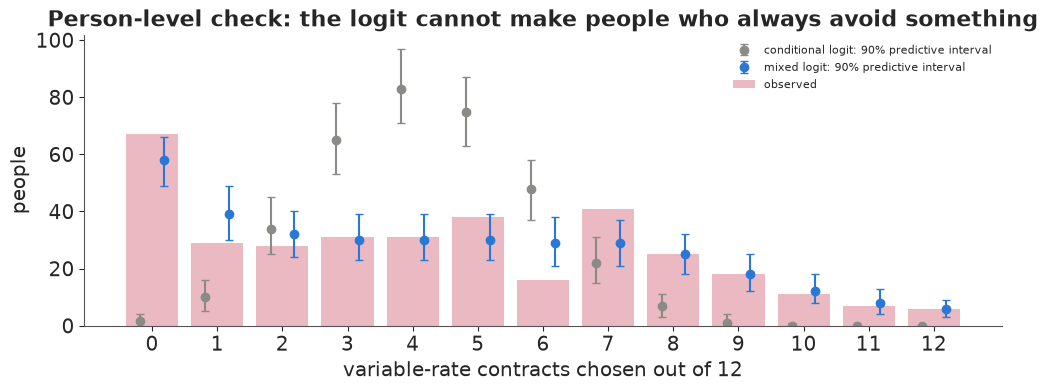
The mixed logit reproduces the shape of the distribution: the pile at zero, the long flat middle and the few people who choose variable rates in 10-12 of their tasks. The observed 67 "never" people sit at the upper edge of its 90% interval (printed above), so the model still slightly underpredicts complete avoidance - a hint that some people may simply never consider these contracts (a mass point, or a non-compensatory screening rule) rather than dislike them by a normally distributed amount. That is a refinement; the logit's failure was of a different order.
5 · Willingness to pay
5.1 · Population WTP: medians, means and tails
B_mixed = population(idata_mixed, True)
bl = az.extract(idata_logit, var_names=["beta"]).to_numpy()          # (attr, sample)
rows = []
for kk, a in enumerate(ATTR[1:], start=1):
    w_logit = -bl[kk] / bl[0]
    w_mixed = -B_mixed[..., kk] / B_mixed[..., 0]
    rows.append({"attribute": LABEL[a],
                 "logit WTP": f"{np.median(w_logit):.2f} [{q(w_logit)[0]:.2f}, {q(w_logit)[2]:.2f}]",
                 "mixed: median person": "{:.2f} [{:.2f}, {:.2f}]".format(*q(np.median(w_mixed, axis=1))[[1, 0, 2]]),
                 "mixed: 10-90% of people": "{:.1f} to {:.1f}".format(*np.median(np.quantile(w_mixed, [0.1, 0.9], axis=1), axis=1)),
                 "mixed: population mean": "{:.2f} [{:.2f}, {:.2f}]".format(*q(w_mixed.mean(axis=1))[[1, 0, 2]])})
wtp_table = pd.DataFrame(rows).set_index("attribute")
print("WTP in c/kWh: posterior median [90% interval]")
wtp_table
WTP in c/kWh: posterior median [90% interval]
| logit WTP | mixed: median person | mixed: 10-90% of people | mixed: population mean | |
|---|---|---|---|---|
| attribute | ||||
| contract length (yr) | -0.17 [-0.20, -0.15] | -0.22 [-0.29, -0.16] | -1.6 to 0.5 | -0.40 [-0.65, -0.19] |
| local company | 2.30 [2.15, 2.48] | 2.82 [2.20, 3.60] | -0.1 to 19.3 | 7.92 [5.74, 11.44] |
| well-known company | 1.59 [1.46, 1.73] | 2.09 [1.65, 2.64] | -0.0 to 12.9 | 5.27 [3.94, 7.52] |
| time-of-day rates | -0.74 [-0.87, -0.61] | -1.15 [-1.73, -0.74] | -12.8 to 3.4 | -3.59 [-6.11, -1.89] |
| seasonal rates | -1.34 [-1.50, -1.19] | -1.39 [-1.88, -1.00] | -11.5 to 1.6 | -3.89 [-6.03, -2.53] |
Read the table row by row for "local company":
- the logit gives one number (about 2.3 c/kWh) with a tight interval, because it assumes everyone is the same;
- the median person in the mixed logit would pay somewhat more (about 2.8 c/kWh; interval in the table);
- but people differ enormously: the middle 80% range from about 0 to 20 c/kWh;
- and the population mean is much larger than the median (around 8 c/kWh) because a lognormal price coefficient has a left tail near zero: a few very price-insensitive people have huge WTPs. Unlike the normal model, this mean exists and has a finite posterior, but it is driven by the tail of an assumed distribution.
Which one to report depends on the question: the median describes a typical customer; the mean is what matters for aggregate welfare or revenue if everyone could be charged their own WTP. For pricing (section 8) we simulate the whole distribution instead of summarising it.
The contract-length row confirms that a long lock-in costs roughly 0.2 c/kWh per year for the median person, and the variable-rate rows that TOD and seasonal contracts must be about 1.2 and 1.4 c/kWh cheaper on average than a fixed one to be equally attractive to the median person.
Published analyses. Train's own mixed-logit analyses of these data (Huber & Train 2001;
the mixed-logit chapters of Train's Discrete Choice Methods with Simulation) use the raw
coding and different distributional choices for price. We have not reproduced their tables and
make no numeric comparison with them here; the verifiable anchor is section 2's maximum-likelihood
conditional logit, which any logit software (e.g. mlogit in R) reproduces on these data.
fig, axes = plt.subplots(1, 3, figsize=(15, 4.2))
bins = np.linspace(-20, 40, 121)
axes[0].hist(wtp_normal.ravel(), bins=bins, density=True, histtype="step", lw=2, color=GREY,
             label="normal price coef.")
axes[0].hist((-B_mixed[..., 2] / B_mixed[..., 0]).ravel(), bins=bins, density=True, histtype="step",
             lw=2, color=BLUE, label="lognormal price coef.")
axes[0].axvline(np.median(-bl[2] / bl[0]), color=ORANGE, lw=2, label="conditional logit")
axes[0].set(xlabel="WTP for a local supplier (c/kWh)", ylabel="density", xlim=(-20, 40),
            title="WTP across people")
axes[0].legend(fontsize=8)
for vals, col, name in [(wtp_normal.mean(axis=1), GREY, "normal"),
                        ((-B_mixed[..., 2] / B_mixed[..., 0]).mean(axis=1), BLUE, "lognormal")]:
    axes[1].hist(np.clip(vals, -30, 30), bins=np.linspace(-30, 30, 61), color=col, alpha=0.6, label=name)
axes[1].set(xlabel="population MEAN WTP, local (c/kWh; clipped at +-30)", ylabel="posterior draws",
            title="Posterior of the population mean")
axes[1].legend(fontsize=8)
# correlation of the random coefficients (lognormal model: first row is log|price coef|)
mu_s, L_s = hyper(idata_mixed, 1000)
cov = np.einsum("sij,skj->sik", L_s, L_s)
sd_s = np.sqrt(np.einsum("sii->si", cov))
corr = (cov / sd_s[:, :, None] / sd_s[:, None, :]).mean(axis=0)
im = axes[2].imshow(corr, cmap="RdBu_r", vmin=-1, vmax=1)
names = ["log|price|", "contract", "local", "known", "tod", "seas"]
axes[2].set_xticks(range(6), names, rotation=45, fontsize=8)
axes[2].set_yticks(range(6), names, fontsize=8)
for i in range(6):
    for j in range(6):
        if i != j:
            axes[2].text(j, i, f"{corr[i, j]:.2f}", ha="center", va="center", fontsize=7)
axes[2].set_title("Taste correlations")
fig.colorbar(im, ax=axes[2], shrink=0.8);
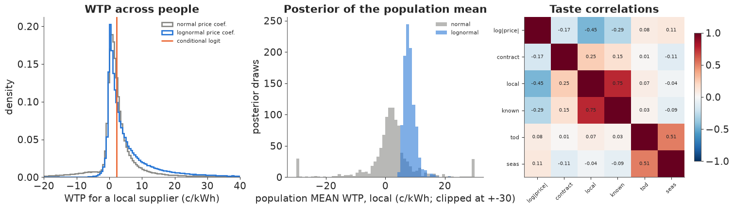
The correlation matrix is worth reading. Liking local and liking well-known suppliers go together strongly (a taste for familiar, trustworthy suppliers). The TOD and seasonal dislikes are positively correlated (a general attitude to variable rates). The price sensitivity (its log magnitude) correlates negatively with the local preference: people who care a lot about local suppliers tend to care less about price, which is precisely what makes the WTP distribution so right-skewed. An independent (diagonal) $\Sigma$ would miss all of this.
5.2 · Individual WTP: how much do 12 answers tell you?
The model also gives each respondent's own posterior. Marketers like "individual-level part-worths"; here is what they look like for the local-supplier WTP.
b_ind = az.extract(idata_mixed, var_names=["beta"], num_samples=400).transpose("sample", ...).to_numpy()
w_ind = -b_ind[..., 2] / b_ind[..., 0]                               # (draw, person)
med_i = np.median(w_ind, axis=0)
lo_i, hi_i = np.quantile(w_ind, [0.05, 0.95], axis=0)
order = np.argsort(med_i)
fig, ax = plt.subplots(figsize=(11, 3.8))
ax.vlines(np.arange(N), lo_i[order], hi_i[order], color=BLUE, alpha=0.35, lw=1.2)
ax.plot(np.arange(N), med_i[order], ".", color=BLUE, ms=3, label="person's posterior median")
ax.axhline(np.median(-bl[2] / bl[0]), color=ORANGE, lw=1.5, label="conditional logit (everyone)")
ax.set(yscale="symlog", ylim=(-30, 200), xlabel="respondents, sorted by posterior median",
       ylabel="WTP, local (c/kWh, symlog)", title="Each respondent's WTP for a local supplier: 90% intervals")
ax.legend(fontsize=8)
width = hi_i - lo_i
print(f"median width of a person's 90% interval: {np.median(width):.1f} c/kWh; "
      f"persons whose interval excludes 0: {np.mean(lo_i > 0):.0%}")
median width of a person's 90% interval: 11.2 c/kWh; persons whose interval excludes 0: 63%
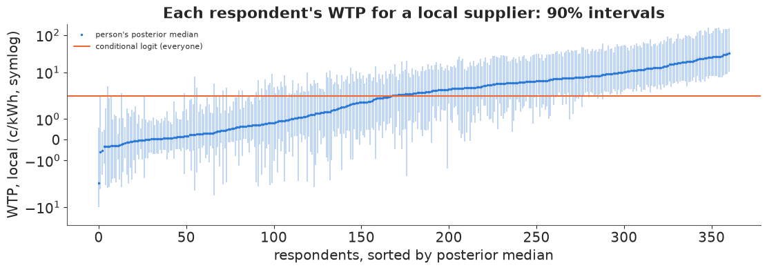
Individual intervals are wide (the typical 90% interval spans about 11 c/kWh) because 12 answers carry little information about six coefficients; only about two thirds of the intervals exclude zero. The ordering is informative - some people are clearly indifferent to local suppliers, others clearly devoted - but a single person's WTP is not a precise number. Use individual posteriors for segmentation or targeting with their uncertainty, never as point estimates.
6 · Model comparison: what does "leave one out" mean here?
6.1 · Leave out a choice task
az.loo on the per-task log-likelihood answers: how well does the model predict a new
answer from a person it has already seen 11 times?
for idt, m in [(idata_normal, m_normal), (idata_mixed, m_lognormal)]:
    with m:
        pm.compute_log_likelihood(idt)
loo_task = {name: az.loo(idt, pointwise=True) for name, idt in
            [("conditional logit", idata_logit), ("mixed, normal price", idata_normal),
             ("mixed, lognormal price", idata_mixed)]}
for name, lo in loo_task.items():
    print(f"{name:>24}: elpd_loo {lo.elpd:8.1f} (se {lo.se:4.1f}), "
          f"tasks with Pareto k > 0.7: {int((lo.pareto_k > 0.7).sum())}")
az.compare(loo_task, round_to=1)
       conditional logit: elpd_loo  -4964.6 (se 41.1), tasks with Pareto k > 0.7: 0
     mixed, normal price: elpd_loo  -3080.6 (se 55.2), tasks with Pareto k > 0.7: 80
mixed, lognormal price: elpd_loo -3060.6 (se 54.8), tasks with Pareto k > 0.7: 110| rank | elpd_diff | dse | p_worse | diag_diff | diag_elpd | p | elpd | se | weight | |
|---|---|---|---|---|---|---|---|---|---|---|
| mixed, lognormal price | 0 | 0.0 | 0.0 | NaN | 110 k̂ > 0.70 | 1068.8 | -3060.6 | 54.8 | 0.9 | |
| mixed, normal price | 1 | -20.0 | 6.7 | 1.0 | 80 k̂ > 0.70 | 1103.0 | -3080.6 | 55.2 | 0.1 | |
| conditional logit | 2 | -1904.0 | 51.3 | 1.0 | 6.0 | -4964.6 | 41.1 | 0.0 |
The mixed logits win by about 1,900 nats - an enormous margin, because knowing a person's other answers makes their next answer much more predictable - and the lognormal price is ahead of the normal one by 15-20 nats (about 3 standard errors; the exact value moves a little from run to run). But two warnings. First, roughly 60-110 tasks have Pareto $k > 0.7$: removing one of only 12 answers can move that person's posterior a lot, and PSIS cannot always approximate it. Second, and more important, this is the right question only if you want to predict known customers. A market simulator is used for new people.
6.2 · Leave out a person
To predict a new person we must leave out all 12 of their answers, and the prediction must integrate over the unknown $\beta_i$:
$$p(y_i \mid \mu, \Sigma) = \int \prod_{t} P(y_{it} \mid \beta)\; \mathcal N(\beta \mid \mu, \Sigma)\, d\beta .$$
Summing the conditional log-likelihood (given the sampled $\beta_i$) by person does not work: $\beta_i$ is informed only by person $i$, so leaving them out changes it completely (you will see $k > 0.7$ for nearly everyone). The integrated likelihood above, used as the pointwise log-likelihood of each person, is the right object (Vehtari et al. 2016 on LOO for latent variable models). It is a 6-dimensional integral per person and posterior draw.
The obvious Monte Carlo estimate is badly biased. Draw $R$ coefficient vectors from $\mathcal N(\mu, \Sigma)$ and average the probabilities of the 12 answers. The product of 12 probabilities is tiny for most draws and large for a few, so the average is dominated by rare draws; with too few, $\log$ of the average is biased down (Jensen). Importance sampling from each person's own posterior (a multivariate-t fitted to their posterior draws of $\beta_i$) puts the draws where the integrand is.
XF = X.reshape(T * J, 6)
M = np.zeros((T, N))
M[np.arange(T), pid] = 1.0                                  # task -> person summation matrix
tasks_of = [np.flatnonzero(pid == i) for i in range(N)]


def naive_person_ll(idata, lognormal_price, S=200, R=200, seed=0):
    """log p(y_i | mu, Sigma) by plain Monte Carlo from the population distribution: (S, N)."""
    mu, L = hyper(idata, S, seed)
    Z = np.random.default_rng(seed).normal(size=(R, 6))
    out = np.empty((S, N))
    for s in range(S):
        B = mu[s] + Z @ L[s].T
        if lognormal_price:
            B[:, 0] = -np.exp(B[:, 0])
        V = (XF @ B.T).reshape(T, J, R)
        lp = V[np.arange(T), y] - special.logsumexp(V, axis=1)          # (task, R)
        out[s] = special.logsumexp(M.T @ lp, axis=1) - np.log(R)
    return out


def is_person_ll(idata, lognormal_price, S=400, R=1000, seed=0, df=5, inflate=1.3):
    """Same integral, importance-sampled from a t fitted to each person's posterior."""
    r = np.random.default_rng(seed)
    b = idata.posterior["beta"].stack(s=("chain", "draw")).transpose("person", "s", "attr").to_numpy().copy()
    if lognormal_price:
        b[..., 0] = np.log(-b[..., 0])                           # back to the normal scale
    m = b.mean(axis=1)
    C = np.einsum("psa,psb->pab", b - m[:, None], b - m[:, None]) / b.shape[1] * inflate**2
    Lq = np.linalg.cholesky(C + 1e-9 * np.eye(6))
    g = r.chisquare(df, (N, R, 1)) / df
    draws = m[:, None] + np.einsum("pab,prb->pra", Lq, r.standard_normal((N, R, 6))) / np.sqrt(g)
    logq = np.array([stats.multivariate_t(m[i], C[i], df=df).logpdf(draws[i]) for i in range(N)])
    loglik = np.empty((N, R))
    for i in range(N):
        B = draws[i].copy()
        if lognormal_price:
            B[:, 0] = -np.exp(B[:, 0])
        V = np.einsum("tja,ra->rtj", X[tasks_of[i]], B)
        loglik[i] = (V[:, np.arange(len(tasks_of[i])), y[tasks_of[i]]]
                     - special.logsumexp(V, axis=2)).sum(axis=1)
    mu, L = hyper(idata, S, seed)
    out = np.empty((S, N))
    for s in range(S):                                           # population density of each draw
        zz = np.linalg.solve(L[s], (draws - mu[s]).reshape(-1, 6).T).T.reshape(N, R, 6)
        logp = -0.5 * (zz**2).sum(-1) - np.log(np.diag(L[s])).sum() - 3 * np.log(2 * np.pi)
        out[s] = special.logsumexp(loglik - logq + logp, axis=1) - np.log(R)
    return out


def loo_from(ll):
    dt = xr.DataTree.from_dict({
        "posterior": xr.Dataset({"dummy": (("chain", "draw"), np.zeros((1, ll.shape[0])))}),
        "log_likelihood": xr.Dataset({"y": (("chain", "draw", "person"), ll[None])})})
    return az.loo(dt, pointwise=True)


t0 = time.time()
ll_naive = naive_person_ll(idata_mixed, True)
ll_is = is_person_ll(idata_mixed, True)
ll_is2 = is_person_ll(idata_mixed, True, R=200, seed=1)
print(f"sum over people of E[log p(y_i | mu, Sigma)]: naive MC (R=200) {ll_naive.mean(0).sum():.0f}, "
      f"importance sampling R=1000 {ll_is.mean(0).sum():.0f}, R=200 (other seed) "
      f"{ll_is2.mean(0).sum():.0f}   [{time.time() - t0:.0f} s]")
sum over people of E[log p(y_i | mu, Sigma)]: naive MC (R=200) -3773, importance sampling R=1000 -3673, R=200 (other seed) -3673 [17 s]
The naive estimate is about 100 nats lower than the importance-sampled one, and the importance-sampled one is stable to a nat between 200 and 1,000 draws and across seeds. (In a prototype, the naive estimate climbed from about -3,773 to -3,685 as $R$ went from 200 to 2,000: still not converged, and 5 times the cost.) A model comparison built on the naive estimate would penalise whichever model has more heterogeneity - exactly the wrong direction.
Now the person-level comparison. For the logit there is nothing to integrate, so summing its task log-likelihood by person is exact.
ll_logit_person = (idata_logit.log_likelihood["y"].stack(s=("chain", "draw")).transpose("s", "task")
                   .to_numpy() @ M)
loo_person = {"conditional logit": loo_from(ll_logit_person[:: ll_logit_person.shape[0] // 400]),
              "mixed, normal price": loo_from(is_person_ll(idata_normal, False)),
              "mixed, lognormal price": loo_from(ll_is)}
for name, lo in loo_person.items():
    print(f"{name:>24}: elpd_loo {lo.elpd:8.1f} (se {lo.se:4.1f}), max Pareto k {float(lo.pareto_k.max()):.2f}")
for lo in list(loo_task.values()) + list(loo_person.values()):
    lo.log_weights = None                      # the big importance-weight matrices (memory)
for idt in (idata_logit, idata_normal, idata_mixed):
    del idt["log_likelihood"]
az.compare(loo_person, round_to=1)
       conditional logit: elpd_loo  -4970.4 (se 57.8), max Pareto k 0.31
     mixed, normal price: elpd_loo  -3694.5 (se 73.1), max Pareto k 0.38
mixed, lognormal price: elpd_loo -3686.5 (se 73.1), max Pareto k 0.40| rank | elpd_diff | dse | p_worse | diag_diff | diag_elpd | p | elpd | se | weight | |
|---|---|---|---|---|---|---|---|---|---|---|
| mixed, lognormal price | 0 | 0.0 | 0.0 | NaN | 27.1 | -3686.5 | 73.1 | 0.7 | ||
| mixed, normal price | 1 | -8.0 | 5.5 | 0.9 | 27.1 | -3694.5 | 73.1 | 0.2 | ||
| conditional logit | 2 | -1283.9 | 66.2 | 1.0 | 17.3 | -4970.4 | 57.8 | 0.0 |
fig, axes = plt.subplots(1, 2, figsize=(12, 3.6))
for (name, lo), col in zip(loo_task.items(), [GREY, ORANGE, BLUE]):
    axes[0].plot(np.sort(np.asarray(lo.pareto_k).ravel()), color=col, label=name)
axes[0].axhline(0.7, color=RED, ls="--", lw=1)
axes[0].set(xlabel="tasks (sorted)", ylabel="Pareto k", title="Leave out one task: PSIS reliability")
axes[0].legend(fontsize=8)
d_person = loo_person["mixed, lognormal price"].elpd_i - loo_person["mixed, normal price"].elpd_i
axes[1].hist(np.asarray(d_person), bins=40, color=BLUE)
axes[1].axvline(0, color="k", lw=1)
axes[1].set(xlabel="elpd per person: lognormal minus normal price", ylabel="people",
            title="Leave out one person: lognormal vs normal price");
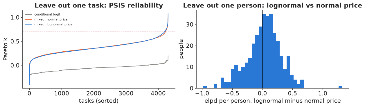
Leaving out whole people, the integrated mixed logits still beat the logit by more than 1,200 nats: taste heterogeneity is a real feature of the population, not only of the individuals already seen. All Pareto $k$ are below 0.5, because a single person moves the population hyperparameters only slightly. Between the two mixed logits the data barely choose: the lognormal price model is ahead by 7-8 nats with a standard error of about 5.5, and per person the differences scatter around zero in both directions. So the case for the lognormal price coefficient is mainly the economic one (section 4.2) - the data do not object to it and lean slightly in its favour.
The two LOOs answer different questions. Here the ranking is the same, but the size of the gaps and the reliability diagnostics are not. Choose the unit you leave out to match the prediction task: new answers from known people (task LOO; e.g. recommending a contract to an existing customer), or new people (person LOO; e.g. market simulation).
7 · A known-truth check (simulated)
Can 12 answers each from 361 people really identify six means, six scales and fifteen correlations? Simulate a new survey on the same design from a known population (the posterior mean of the fitted hyperparameters), refit, and compare.
mu_true = idata_mixed.posterior["mu"].mean(("chain", "draw")).to_numpy()
L_true = np.zeros((6, 6))
L_true[tri] = idata_mixed.posterior["chol"].mean(("chain", "draw")).to_numpy()
rs = np.random.default_rng(2068)
B_true = mu_true + rs.normal(size=(N, 6)) @ L_true.T
B_true[:, 0] = -np.exp(B_true[:, 0])
p_sim = special.softmax(np.einsum("tja,ta->tj", X, B_true[pid]), axis=1)
y_sim = (p_sim.cumsum(axis=1) > rs.uniform(size=(T, 1))).argmax(axis=1)
idata_sim = fit(mixed_logit(True, y_=y_sim))
sd_true = np.sqrt((L_true**2).sum(axis=1))
raw_true = B_true.copy()
raw_true[:, 0] = np.log(-raw_true[:, 0])                  # the 361 simulated people, normal scale
mean_realised, sd_realised = raw_true.mean(axis=0), raw_true.std(axis=0)
cov_true = L_true @ L_true.T
corr_true = cov_true / np.outer(sd_true, sd_true)
mu_sim, L_sim = hyper(idata_sim, 1000)
cov_sim = np.einsum("sij,skj->sik", L_sim, L_sim)
sd_sim = np.sqrt(np.einsum("sii->si", cov_sim))
corr_sim = cov_sim / sd_sim[:, :, None] / sd_sim[:, None, :]

fig, axes = plt.subplots(1, 3, figsize=(14, 3.6))
for ax, draws, truth, realised, title in [(axes[0], mu_sim, mu_true, mean_realised, "means mu"),
                                          (axes[1], sd_sim, sd_true, sd_realised, "scales")]:
    lo, med, hi = np.quantile(draws, [0.05, 0.5, 0.95], axis=0)
    ax.errorbar(range(6), med, yerr=[med - lo, hi - med], fmt="o", color=BLUE, capsize=3, label="posterior 90%")
    ax.plot(range(6), truth, "x", color=RED, ms=9, mew=2, label="population truth")
    ax.plot(range(6), realised, "+", color="k", ms=10, mew=1.5, label="the 361 simulated people")
    ax.set_xticks(range(6), names, rotation=30, fontsize=8)
    ax.set_title(f"Simulated survey: {title}")
    ax.legend(fontsize=8)
iu = np.triu_indices(6, 1)
lo, med, hi = np.quantile(corr_sim[:, iu[0], iu[1]], [0.05, 0.5, 0.95], axis=0)
axes[2].errorbar(corr_true[iu], med, yerr=[med - lo, hi - med], fmt="o", color=BLUE, capsize=2)
axes[2].plot([-1, 1], [-1, 1], color="k", lw=1)
axes[2].set(xlabel="true correlation", ylabel="posterior median (90%)", title="the 15 correlations")
covered = np.mean((np.quantile(corr_sim[:, iu[0], iu[1]], 0.05, axis=0) <= corr_true[iu])
                  & (corr_true[iu] <= np.quantile(corr_sim[:, iu[0], iu[1]], 0.95, axis=0)))
print(f"90% intervals covering the truth: means {np.mean((q(mu_sim, (0.05,), axis=0)[0] <= mu_true) & (mu_true <= q(mu_sim, (0.95,), axis=0)[0])):.0%}, "
      f"scales {np.mean((np.quantile(sd_sim, 0.05, axis=0) <= sd_true) & (sd_true <= np.quantile(sd_sim, 0.95, axis=0))):.0%}, "
      f"correlations {covered:.0%}")
print("posterior median / truth:", np.round(np.median(mu_sim, axis=0) / mu_true, 2), "(means),",
      np.round(np.median(sd_sim, axis=0) / sd_true, 2), "(scales)")
print("realised / truth       :", np.round(mean_realised / mu_true, 2), "(means),",
      np.round(sd_realised / sd_true, 2), "(scales)")
del idata_sim, cov_sim, corr_sim
sampled in 16 s; divergences 0; max tree depth 5; r_hat max (mu, chol, z) 1.029; bulk ESS min (mu, chol) 185
90% intervals covering the truth: means 67%, scales 67%, correlations 93%
posterior median / truth: [1.77 1.09 1.15 1.18 1.08 0.95] (means), [1.25 1.07 1.13 1.11 1.05 0.95] (scales)
realised / truth       : [1.43 1.   1.1  1.1  1.1  1.02] (means), [1.04 1.03 1.08 1.07 1.03 1.  ] (scales)
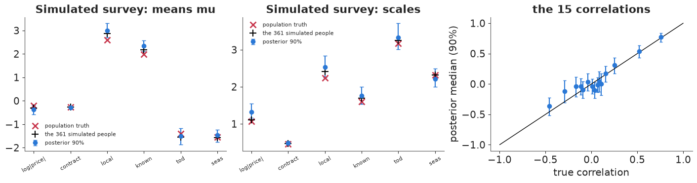
Two of the six means (local, well-known) and two of the six scales (log|price|, local) miss the population truth (red crosses) with their 90% intervals, all on the high side. For the two means the black crosses explain most of it: the 361 simulated people happen to like local and well-known suppliers about 10% more than the population they were drawn from, and the posterior follows the people it has seen. The spread of log|price| is overestimated by about 25% even relative to the simulated people, so price heterogeneity is the least well pinned-down part of the model. One simulated survey cannot tell a small systematic bias from bad luck; that needs many replications (e.g. simulation-based calibration). The correlations are recovered well: the three large ones we interpreted (local with well-known, TOD with seasonal, price with local) are clearly identified, and the small ones shrink towards zero as the LKJ(2) prior intends. No parameter is unidentified.
8 · Substitution patterns and a market simulator
8.1 · A market
To use the model we need a market. We define one (an assumption, not data): three existing offers, all within the price range of the survey (7-9 c/kWh).
| competitor | price | contract | local | well-known | rates |
|---|---|---|---|---|---|
| Incumbent | 9c | none | yes | yes | fixed |
| National discounter | 7c | 5 years | no | yes | fixed |
| Incumbent TOD plan | 8c average | none | yes | yes | time-of-day |
A new entrant, neither local nor known, considers a fixed-price offer. Market shares come from the model in two ways: the logit uses one $\beta$ per posterior draw; the mixed logit simulates 1,000 customers from $\mathcal N(\mu, \Sigma)$ for each posterior draw and averages their choice probabilities, so both parameter uncertainty and taste heterogeneity are in the shares. Like the survey, the market has no "stay with my current supplier" option: shares are among customers who pick one of these offers.
competitors = pd.DataFrame(
    [[9, 0, 1, 1, 0, 0], [7, 5, 0, 1, 0, 0], [8, 0, 1, 1, 1, 0]], columns=ATTR,
    index=["Incumbent", "National discounter", "Incumbent TOD"], dtype=float)
C = competitors.to_numpy()
S_MKT, R_MKT = 300, 1000
beta_logit_mkt = bl[:, np.random.default_rng(3).choice(bl.shape[1], S_MKT, replace=False)].T
B_mkt = population(idata_mixed, True, S=S_MKT, R=R_MKT, seed=3)          # (S, R, 6)


def shares(profiles, model):
    """profiles (K, 6) -> posterior draws of market shares (S, K)."""
    if model == "logit":
        return special.softmax(beta_logit_mkt @ profiles.T, axis=1)
    return special.softmax(np.einsum("sra,ka->srk", B_mkt, profiles), axis=2).mean(axis=1)


base = {m: shares(C, m) for m in ["logit", "mixed"]}
print(pd.DataFrame({m: [f"{v:.1%}" for v in base[m].mean(axis=0)] for m in base}, index=competitors.index))
                     logit  mixed
Incumbent            37.4%  38.7%
National discounter  18.1%  24.6%
Incumbent TOD        44.5%  36.7%
8.2 · Where does the entrant's share come from?
Add the entrant at 8c with a 1-year contract and compute diversion ratios: of every customer the entrant wins, what fraction came from each competitor? Then the red-bus test: add an exact clone of the national discounter.
entrant = np.array([8, 1, 0, 0, 0, 0], float)
rows = []
for m in ["logit", "mixed"]:
    s1 = shares(np.vstack([C, entrant]), m)
    div = (base[m] - s1[:, :3]) / s1[:, [3]]
    s_clone = shares(np.vstack([C, C[1]]), m)
    rows.append({"model": m, "entrant share": s1[:, 3].mean(),
                 **{f"from {c}": v for c, v in zip(competitors.index, div.mean(axis=0))},
                 "discounter alone": base[m][:, 1].mean(),
                 "discounter + clone": (s_clone[:, 1] + s_clone[:, 3]).mean()})
subst = pd.DataFrame(rows).set_index("model")
subst.round(3)
| entrant share | from Incumbent | from National discounter | from Incumbent TOD | discounter alone | discounter + clone | |
|---|---|---|---|---|---|---|
| model | ||||||
| logit | 0.052 | 0.374 | 0.181 | 0.445 | 0.181 | 0.306 |
| mixed | 0.063 | 0.343 | 0.481 | 0.177 | 0.246 | 0.296 |
fig, axes = plt.subplots(1, 2, figsize=(12, 3.8))
w = 0.38
for i, (m, col) in enumerate([("logit", GREY), ("mixed", BLUE)]):
    axes[0].bar(np.arange(3) + (i - 0.5) * w, subst.loc[m, [f"from {c}" for c in competitors.index]],
                width=w, color=col, label=f"{m}: diversion")
    axes[0].scatter(np.arange(3) + (i - 0.5) * w, base[m].mean(axis=0), marker="_", s=400, color="k",
                    zorder=3, label="baseline share" if i == 0 else None)
axes[0].set_xticks(range(3), ["Incumbent", "National\ndiscounter", "Incumbent\nTOD"])
axes[0].set(ylabel="share of the entrant's customers", title="Who loses customers to the entrant?")
axes[0].legend(fontsize=8)
for i, (m, col) in enumerate([("logit", GREY), ("mixed", BLUE)]):
    axes[1].bar(i - 0.2, subst.loc[m, "discounter alone"], width=0.4, color=col, alpha=0.5)
    axes[1].bar(i + 0.2, subst.loc[m, "discounter + clone"], width=0.4, color=col)
    axes[1].text(i + 0.2, subst.loc[m, "discounter + clone"] + 0.005,
                 f"+{subst.loc[m, 'discounter + clone'] / subst.loc[m, 'discounter alone'] - 1:.0%}",
                 ha="center", fontsize=9)
axes[1].set_xticks([0, 1], ["logit", "mixed logit"])
axes[1].set(ylabel="combined market share", title="Red bus / blue bus: add an identical clone\n(light: alone, dark: with clone)");
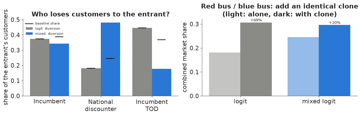
Under the logit, diversion ratios are exactly the baseline shares (IIA): the entrant, a non-local fixed-price supplier, is assumed to steal most from the local incumbent TOD plan simply because it is the biggest. The mixed logit disagrees: the entrant takes a much larger share of its customers from the national discounter, the other non-local fixed-price offer, because the people who already choose non-local fixed contracts are the ones who do not care much about "local" and dislike variable rates.
The clone test shows the same thing more starkly. A perfect copy of the discounter should add almost nothing - its customers were already served. The logit has the pair's share jump by roughly 70%; the mixed logit by about 20%. The mixed logit reduces the red-bus problem but does not remove it: conditional on $\beta_i$ each person still has independent Gumbel errors for the two identical offers. Removing it entirely needs correlated errors between similar alternatives (nested logit, or an error component in the mixed logit - see "Try it yourself").
8.3 · The pricing decision
The entrant's margin is its price minus a wholesale cost of 6 c/kWh (an assumption for illustration). Expected profit per kWh of the whole market is share $\times$ (price - 6). We scan price and contract length. Prices outside 7-9 c/kWh are extrapolation beyond the survey and are shaded.
COST = 6.0
prices = np.arange(6.5, 10.01, 0.25)
profit = {}
for cl in [0, 1, 5]:
    for m in ["logit", "mixed"]:
        sh = np.stack([shares(np.vstack([C, [p, cl, 0, 0, 0, 0]]), m)[:, 3] for p in prices])
        profit[(m, cl)] = sh * (prices[:, None] - COST)                  # (price, draw)

fig, axes = plt.subplots(1, 2, figsize=(13, 4))
for ax, m in zip(axes, ["logit", "mixed"]):
    for cl, col in zip([0, 1, 5], [BLUE, ORANGE, AQUA]):
        pr = 100 * profit[(m, cl)]
        lo, med, hi = np.quantile(pr, [0.05, 0.5, 0.95], axis=1)
        ax.fill_between(prices, lo, hi, color=col, alpha=0.2)
        ax.plot(prices, pr.mean(axis=1), color=col, lw=2, label=f"{cl}-year contract")
        ax.plot(prices[pr.mean(axis=1).argmax()], pr.mean(axis=1).max(), "o", color=col, ms=8)
    for x0, x1 in [(6.5, 7), (9, 10)]:
        ax.axvspan(x0, x1, color=GREY, alpha=0.12)
    ax.set(xlabel="entrant's fixed price (c/kWh)", ylabel="expected margin (c per 100 kWh of market)",
           title=f"{'Conditional logit' if m == 'logit' else 'Mixed logit'}: expected margin, 90% band")
    ax.legend(fontsize=8)

best = {}
for (m, cl), pr in profit.items():
    i = pr.mean(axis=1).argmax()
    best[(m, cl)] = (prices[i], pr.mean(axis=1)[i])
print("expected-margin-maximising price by model and contract length:")
print(pd.DataFrame([{"model": m, "contract (yr)": cl, "best price": p, "E[margin] c/100kWh": 100 * v}
                    for (m, cl), (p, v) in best.items()]).set_index(["model", "contract (yr)"]).round(2))
expected-margin-maximising price by model and contract length:
                     best price  E[margin] c/100kWh
model contract (yr)
logit 0                    7.75               11.75
mixed 0                    7.25               18.52
logit 1                    7.75               10.62
mixed 1                    7.00               15.71
logit 5                    7.75                7.03
mixed 5                    6.75                9.37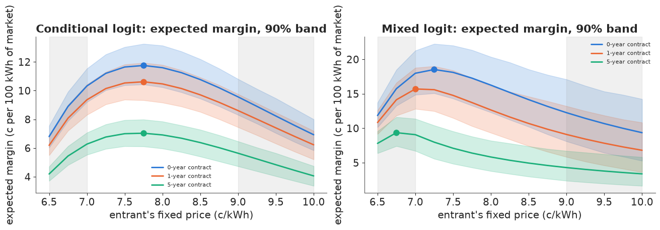
The two models give different advice. The logit puts the best price at 7.75 c/kWh for every contract length; the mixed logit at 7.25 without a contract (7.0 and 6.75 with 1- and 5-year contracts), and it expects a higher margin at its optimum. Its bands are also much wider: taste heterogeneity is uncertain, and it matters for shares. One reading of the lower price: with heterogeneous tastes the entrant's natural customers are the not-local-minded people currently with the discounter, who are already choosing on price, so it pays to compete on price for them rather than charge a premium to everyone. Both models agree that no contract is best: every year of lock-in costs the entrant customers.
How much would the entrant lose by following the logit? Evaluate the logit's recommendation under the (better-supported) mixed logit, draw by draw.
p_logit, _ = best[("logit", 0)]
p_mixed, _ = best[("mixed", 0)]
pm_ = profit[("mixed", 0)]
gain = pm_[np.argmin(np.abs(prices - p_mixed))] - pm_[np.argmin(np.abs(prices - p_logit))]
print(f"mixed-logit optimum {p_mixed:.2f}c vs logit optimum {p_logit:.2f}c (no contract): "
      f"margin gain {100 * gain.mean():.2f} c/100kWh, 90% interval {q(100 * gain)[[0, 2]]}, "
      f"P(gain > 0) = {np.mean(gain > 0):.2f}")
print(f"relative to the logit's price: {gain.mean() / pm_[np.argmin(np.abs(prices - p_logit))].mean():+.0%}")
mixed-logit optimum 7.25c vs logit optimum 7.75c (no contract): margin gain 1.25 c/100kWh, 90% interval [-0.1   2.58], P(gain > 0) = 0.94
relative to the logit's price: +7%
Under the mixed logit, pricing at 7.25 instead of 7.75 raises the expected margin by about 7%, with probability about 0.9 of being an improvement. The margin curve is flat near its peak, so this is a modest gain, not a dramatic one; what changes more is the story of whom the entrant competes with, which matters for how the discounter might respond.
Caveats a pricing team should hear. Stated preferences are hypothetical: people may overstate their dislike of variable rates or their love of local firms (hypothetical bias). The survey has no "no switch" option, so these are shares among switchers, not of all households. The market is invented, the cost is assumed, and competitors will react. The model's job is to make the trade-offs explicit and carry the uncertainty through, not to replace these judgements.
Summary
- The logit is a softmax over alternatives of a linear utility; in PyMC it is a
(task, alt, attr)array andpm.Categorical(logit_p=...). Priors must be checked on the choice scale: "vague" coefficients mean deterministic choices. - IIA is a property of one person with fixed tastes. A person-level predictive check on the panel (67 people never chose a variable-rate contract; the logit expects one or two) shows that the population is not one person.
- The mixed logit (non-centred person effects, LKJ covariance) reproduces the person-level pattern and reveals correlated tastes. A normal price coefficient fits and samples fine but makes one in nine people like higher prices and gives WTP a distribution with no mean; a lognormal price coefficient fixes this; LOO leans its way only slightly (about 8 +- 5.5 nats leaving out people).
- WTP: the median person values a local supplier at roughly 3 c/kWh, but the middle 80% of people range from about 0 to 20 c/kWh; means are tail-driven; individual WTPs from 12 answers are very uncertain.
- LOO for panels: leave out the unit you want to predict. Leaving out people needs the integrated likelihood, and a naive simulated integral was off by about 100 nats; importance sampling from each person's posterior fixed it.
- Decision: the mixed logit's substitution patterns (the entrant takes from the similar discounter, not in proportion to shares) change the recommended price from 7.75 to 7.25 c/kWh, with no contract, for about 7% more expected margin.
Try it yourself
- WTP space. Reparameterise the mixed logit directly in willingness to pay (Train & Weeks 2005): $U = \lambda_i(-\text{price} + w_i^\top x)$ with $\lambda_i$ lognormal and $w_i$ normal. Put priors on WTP directly. Does the population mean WTP for "local" become less tail-driven, and does person-level LOO change?
- An error component for the clone. Add a normal error term, drawn afresh in every choice task, shared by the "non-local fixed-price" alternatives of that task (an error component that mimics a nest), and repeat the red-bus test of 8.2. How much of the clone's extra share disappears, and does the entrant's diversion change?
- A mass point of refusers. Section 4.3's check showed slightly too few people who never
choose variable rates. Add a latent class "never considers TOD/seasonal" (a two-component
mixture per person, marginalised with
pt.logsumexpover the person's 12 answers). What share of people are in it, and does the pricing of a TOD offer change?