Who is right when nobody knows the answer?
Seven experienced pathologists look at the same 118 slides of cervical tissue and each says "carcinoma" or "no carcinoma". On 34 slides all seven say no, on 16 all seven say yes, and on the remaining 68 they disagree. There is no gold standard: no biopsy follow-up, no consensus panel, nothing but the seven opinions.
The same situation is everywhere: several imperfect diagnostic tests for a disease with no perfect test (tuberculosis, Lyme disease, many veterinary infections), crowdworkers labelling images or sentences for machine learning, reviewers scoring grant proposals, radiologists reading the same scans. The questions are always the same:
- What is the true label of each item, and how sure can we be?
- How good is each rater (sensitivity, specificity, a whole confusion matrix)?
- What is the prevalence of each class?
- What should we do: which items deserve an expensive expert opinion, and which raters are worth paying for?
The obvious answer, majority vote, answers only question 1, badly. The model-based answer treats the true label as a latent class and the raters as noisy measurements of it (Dawid & Skene 1979; Hui & Walter 1980). It can answer all four questions, but only under assumptions that the data can partly check and partly cannot. This notebook is about both.
| part | data | question |
|---|---|---|
| 1-2 | carcinoma | what does majority vote assume? |
| 3 | carcinoma | the two-class latent class model; label switching |
| 4-5 | carcinoma | is conditional independence plausible? random effects and a third class |
| 6 | simulated + carcinoma | when can a model without a gold standard answer at all? |
| 7-8 | anaesthetists (+ simulated) | K = 4 categories: Dawid-Skene with pooled confusion matrices |
| 9 | carcinoma | decisions: adjudication and which raters to keep |
import logging
import time
import warnings
from itertools import combinations

import arviz as az
import matplotlib.pyplot as plt
import numpy as np
import pandas as pd
import pymc as pm
import pytensor
import pytensor.tensor as pt
import xarray as xr
from scipy import special, stats

from pymc_challenges import data

RANDOM_SEED = 69
rng = np.random.default_rng(RANDOM_SEED)
az.style.use("arviz-variat")
logging.getLogger("pymc").setLevel(logging.WARNING)  # many small fits: no sampler banner each
warnings.filterwarnings("ignore", category=RuntimeWarning, module="arviz")
warnings.filterwarnings("ignore", message=".*effective sample size per chain.*")
BLUE, ORANGE, AQUA, GREY, PURPLE, RED = "#2a78d6", "#eb6834", "#1baf7a", "#8a8a86", "#8c5ac8", "#c8384e"
print(f"PyMC {pm.__version__}, ArviZ {az.__version__}, PyTensor {pytensor.__version__}")


def q(x, probs=(0.05, 0.5, 0.95), axis=None):
    """Posterior quantiles, rounded for printing."""
    return np.round(np.quantile(x, probs, axis=axis), 3)


def draws(idata, var):
    """Posterior draws of one variable as a NumPy array with (chain*draw) first."""
    da = idata.posterior[var]
    return da.stack(s=("chain", "draw")).transpose("s", ...).to_numpy()


def diag(idata, var_names):
    """Divergences, worst r_hat and smallest bulk ESS over the listed variables."""
    rh = max(float(az.rhat(idata.posterior[v]).max()) for v in var_names)
    es = min(float(az.ess(idata.posterior[v]).min()) for v in var_names)
    return (f"divergences {int(idata.sample_stats['diverging'].sum())}, max r_hat {rh:.3f}, "
            f"min bulk ESS {es:.0f}")
PyMC 6.3.2, ArviZ 1.3.0, PyTensor 3.3.2
1 · Seven pathologists, 118 slides
data.describe("carcinoma_pathologists")
carc = data.load("carcinoma_pathologists")
RATERS = list("ABCDEFG")
Y = (carc[RATERS].to_numpy() == 2).astype(int)          # 1 = "carcinoma"
N, J = Y.shape
k_pos = Y.sum(axis=1)                                    # positive calls per slide
patterns, pat_count = np.unique(Y, axis=0, return_counts=True)
print(f"{N} slides x {J} pathologists; {len(patterns)} distinct patterns of the {2**J} possible")
print("share of slides called positive by each pathologist:",
      dict(zip(RATERS, Y.mean(axis=0).round(2).tolist())))
print("slides by number of positive calls:", np.bincount(k_pos).tolist(), "(0, 1, ..., 7 calls)")
carcinoma_pathologists: Seven pathologists (A-G) each classified the same 118 slides of the uterine cervix for carcinoma (in situ or invasive). One row per slide: slide (1-118), A..G (1 = no carcinoma, 2 = carcinoma). There is no gold standard; 20 distinct rating patterns occur.
  source: Holmquist, McMahan & Williams (1967, Archives of Pathology), as dichotomised in Landis & Koch (1977, Biometrics 33:363-374) and Agresti (2002, Categorical Data Analysis, Table 13.1); distributed as `carcinoma` in the CRAN package poLCA (GPL >= 2; the URL). CONVERTED from the .rda with R (values unchanged, a slide index added) - keep the CSV in data/.
  url:    https://raw.githubusercontent.com/cran/poLCA/master/data/carcinoma.rda
118 slides x 7 pathologists; 20 distinct patterns of the 128 possible
share of slides called positive by each pathologist: {'A': 0.56, 'B': 0.67, 'C': 0.38, 'D': 0.27, 'E': 0.6, 'F': 0.21, 'G': 0.56}
slides by number of positive calls: [34, 10, 7, 8, 9, 16, 18, 16] (0, 1, ..., 7 calls)
Pathologists differ a lot in how often they say "carcinoma": B calls 67% of the slides positive, F only 21%. Either the slides B and F looked at differ (they did not - everyone saw all 118) or they have different thresholds. Only 20 of the 128 possible patterns occur, which already says the opinions are far from random.
Agreement between two raters is usually summarised by Cohen's kappa, the agreement beyond what their marginal rates would produce by chance: $\kappa = (p_o - p_e)/(1 - p_e)$.
pairs = list(combinations(range(J), 2))


def kappa(a, b):
    po = np.mean(a == b)
    pe = a.mean() * b.mean() + (1 - a.mean()) * (1 - b.mean())
    return (po - pe) / (1 - pe)


K_mat = np.eye(J)
for a, b in pairs:
    K_mat[a, b] = K_mat[b, a] = kappa(Y[:, a], Y[:, b])

order = np.lexsort((Y @ 2 ** np.arange(J)[::-1], k_pos))   # by score, then pattern
fig, axes = plt.subplots(1, 3, figsize=(15, 4.4), width_ratios=[2.2, 1, 1.2])
axes[0].imshow(Y[order].T, aspect="auto", cmap="Greys", interpolation="nearest")
axes[0].set_yticks(range(J), RATERS)
axes[0].set(xlabel="slide (sorted by number of positive calls)", ylabel="pathologist",
            title="Every slide's seven calls (black = carcinoma)")
for x in np.cumsum(np.bincount(k_pos))[:-1]:
    axes[0].axvline(x - 0.5, color=ORANGE, lw=0.8)
axes[1].barh(range(J), Y.mean(axis=0), color=BLUE)
axes[1].set_yticks(range(J), RATERS)
axes[1].invert_yaxis()
axes[1].set(xlabel="share of slides called positive", title="Thresholds differ")
im = axes[2].imshow(np.where(np.eye(J, dtype=bool), np.nan, K_mat), cmap="viridis", vmin=0, vmax=1)
axes[2].set_xticks(range(J), RATERS)
axes[2].set_yticks(range(J), RATERS)
for a, b in pairs:
    for (r, c) in [(a, b), (b, a)]:
        axes[2].text(c, r, f"{K_mat[a, b]:.2f}", ha="center", va="center", fontsize=7,
                     color="w" if K_mat[a, b] < 0.6 else "k")
axes[2].set_title("Cohen's kappa between pairs")
fig.colorbar(im, ax=axes[2], shrink=0.8);
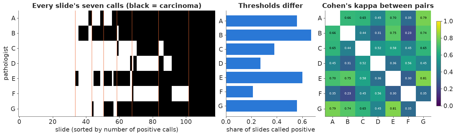
Kappa ranges from about 0.2 (B with F: one says yes to almost everything, the other to almost nothing) to about 0.8. Kappa describes agreement; it does not say who is right. To talk about accuracy we need a model of the truth.
2 · Majority vote, and what it assumes
With seven raters the majority is always defined. Majority vote calls a slide positive when four or more pathologists do:
mv = (k_pos >= 4).astype(int)
agree_mv = (Y == mv[:, None])
mv_se = (Y[mv == 1] == 1).mean(axis=0)
mv_sp = (Y[mv == 0] == 0).mean(axis=0)
print(f"majority vote: {mv.sum()} of {N} slides positive ({mv.mean():.0%})")
print(pd.DataFrame({"agreement with MV": agree_mv.mean(axis=0), "'sensitivity' vs MV": mv_se,
                    "'specificity' vs MV": mv_sp}, index=RATERS).round(2).T)
majority vote: 59 of 118 slides positive (50%)
                        A     B     C     D     E     F     G
agreement with MV    0.94  0.81  0.88  0.77  0.88  0.71  0.94
'sensitivity' vs MV  1.00  0.98  0.76  0.54  0.98  0.42  1.00
'specificity' vs MV  0.88  0.64  1.00  1.00  0.78  1.00  0.88
Majority vote is itself a model, with three silent assumptions:
- every rater is equally good (B, who says yes to two thirds of slides, gets the same vote as F, who says yes to one fifth);
- errors are symmetric (a false positive is as likely as a false negative);
- the label is certain: a 4-3 slide is as positive as a 7-0 slide.
The "sensitivity against the majority" table is also circular: each rater is part of the majority it is scored against, and the majority's own mistakes are counted as the rater's. Section 8 measures, on simulated data where the truth is known, how much accuracy majority vote leaves on the table.
3 · The two-class latent class model
3.1 · The model
Let $D_i \in \{0, 1\}$ be the unobserved true status of slide $i$, with prevalence $\pi = P(D_i = 1)$. Rater $j$ has sensitivity $\mathrm{Se}_j = P(y_{ij} = 1 \mid D_i = 1)$ and specificity $\mathrm{Sp}_j = P(y_{ij} = 0 \mid D_i = 0)$. The key assumption is conditional independence: given the true status, the raters err independently. Then
$$p(y_i) = \pi \prod_j \mathrm{Se}_j^{y_{ij}} (1 - \mathrm{Se}_j)^{1 - y_{ij}} + (1 - \pi) \prod_j (1 - \mathrm{Sp}_j)^{y_{ij}} \mathrm{Sp}_j^{1 - y_{ij}} .$$
The discrete $D_i$ never enters the sampler: we sum it out on the log scale with
pt.logaddexp (a two-term logsumexp). Afterwards the posterior probability that slide $i$
is positive is the share of that sum contributed by the first term,
$P(D_i = 1 \mid y_i) = \pi\, p(y_i \mid D = 1) / p(y_i)$, averaged over the posterior.
Can the data identify it? With $J$ binary raters the data are a multinomial over $2^J$ patterns: $2^J - 1$ free cell probabilities ("degrees of freedom"). The model has $2J + 1$ parameters. Necessary for identification: $2^J - 1 \ge 2J + 1$, i.e. at least three raters (7 = 7 with three raters, just identified; here $127 \gg 15$). Section 6 returns to this.
3.2 · A first attempt, and label switching
The model has an exact symmetry. Rename "diseased" as "healthy" and replace $(\pi, \mathrm{Se}_j, \mathrm{Sp}_j)$ by $(1 - \pi, 1 - \mathrm{Sp}_j, 1 - \mathrm{Se}_j)$: the likelihood is unchanged. With symmetric priors (Beta(1, 1) on everything) the posterior has two mirror-image modes, in one of which the pathologists are worse than a coin flip. We start four chains at two different points, as one should when checking convergence.
def lcm2(Y_, youden=True, se_prior=None, sp_prior=None):
    """Two-class latent class model with conditional independence.

    youden=True parameterises Se_j = fpr_j + (1 - fpr_j) * u_j, so Se_j > 1 - Sp_j (every rater
    better than chance). youden=False puts Beta priors on Se_j and Sp_j directly; se_prior /
    sp_prior map a rater index to the (a, b) of an informative Beta (default Beta(1, 1)).
    """
    R = Y_.shape[1]
    se_ab = np.array([(se_prior or {}).get(j, (1.0, 1.0)) for j in range(R)])
    sp_ab = np.array([(sp_prior or {}).get(j, (1.0, 1.0)) for j in range(R)])
    with pm.Model(coords={"rater": np.arange(R), "item": np.arange(len(Y_))}) as m:
        pi = pm.Beta("pi", 1.0, 1.0)
        fpr = pm.Beta("fpr", sp_ab[:, 1], sp_ab[:, 0], dims="rater")   # fpr = 1 - Sp
        if youden:
            u = pm.Beta("u", 1.0, 1.0, dims="rater")
            se = pm.Deterministic("se", fpr + (1 - fpr) * u, dims="rater")
        else:
            se = pm.Beta("se", se_ab[:, 0], se_ab[:, 1], dims="rater")
        pm.Deterministic("sp", 1 - fpr, dims="rater")
        l1 = pt.log(pi) + (Y_ * pt.log(se) + (1 - Y_) * pt.log1p(-se)).sum(axis=1)
        l0 = pt.log1p(-pi) + (Y_ * pt.log(fpr) + (1 - Y_) * pt.log1p(-fpr)).sum(axis=1)
        ll = pt.logaddexp(l1, l0)                     # D summed out
        pm.Potential("lik", ll.sum())
        pm.Deterministic("ll", ll, dims="item")
        pm.Deterministic("p_pos", pt.exp(l1 - ll), dims="item")
    return m


mirror = [{"pi": 0.4, "se": np.full(J, 0.8), "fpr": np.full(J, 0.2)},
          {"pi": 0.6, "se": np.full(J, 0.2), "fpr": np.full(J, 0.8)}] * 2
t0 = time.time()
with lcm2(Y, youden=False):
    # a per-chain list of initvals runs PyMC's own NUTS (multiprocess: cores=2)
    idata_sw = pm.sample(nuts_sampler="pymc", initvals=mirror, chains=4, cores=2,
                         random_seed=RANDOM_SEED, progressbar=False)
print(f"{time.time() - t0:.0f} s; {diag(idata_sw, ['pi', 'se', 'sp'])}")
print("per-chain posterior means:")
print(pd.DataFrame({"pi": idata_sw.posterior["pi"].mean("draw"),
                    "Se[A]": idata_sw.posterior["se"].sel(rater=0).mean("draw"),
                    "Sp[A]": idata_sw.posterior["sp"].sel(rater=0).mean("draw"),
                    "Se[F]": idata_sw.posterior["se"].sel(rater=5).mean("draw")}).round(2))
2 s; divergences 0, max r_hat 1.738, min bulk ESS 6
per-chain posterior means:
     pi  Se[A]  Sp[A]  Se[F]
0  0.53   0.95   0.88   0.41
1  0.47   0.12   0.05   0.02
2  0.53   0.95   0.88   0.40
3  0.47   0.12   0.06   0.02
Chains 0 and 2 found pathologist A with sensitivity about 0.95; chains 1 and 3 found 0.12, the mirror image (and F's sensitivity 0.40 vs 0.02). Each chain is a healthy sample of its own mode (no divergences), and the two modes describe the data equally well. The pooled r_hat is 1.7 with a bulk ESS of 6. The prevalence barely shows it (0.53 vs 0.47), because $\pi$ happens to sit near 1/2 - a warning against checking convergence on one convenient parameter.
Starting all chains near the centre of the prior, as nutpie does by default, can easily put all four in the same mode. The posterior would still be bimodal; one would just not see it.
3.3 · The fix: raters better than chance
The mirror mode is not a different scientific hypothesis, it is a relabelling. We remove it with a constraint that is true by assumption for any rater worth modelling: a rater says "yes" more often to diseased slides than to healthy ones, $\mathrm{Se}_j > 1 - \mathrm{Sp}_j$ (positive Youden index $\mathrm{Se} + \mathrm{Sp} - 1$). The parameterisation
$$\mathrm{fpr}_j = 1 - \mathrm{Sp}_j \sim \mathrm{Beta}(1, 1), \qquad \mathrm{Se}_j = \mathrm{fpr}_j + (1 - \mathrm{fpr}_j)\, u_j, \quad u_j \sim \mathrm{Beta}(1, 1)$$
builds the constraint in, and removes the mirror mode entirely. What does it imply before seeing data? Simulate the prior predictive number of positive calls per slide:
S = 4000
pr = np.random.default_rng(1)
pi_p = pr.beta(1, 1, S)
fpr_p = pr.beta(1, 1, (S, J))
se_p = fpr_p + (1 - fpr_p) * pr.beta(1, 1, (S, J))
D_p = pr.random(S) < pi_p
kp_prior = (pr.random((S, J)) < np.where(D_p[:, None], se_p, fpr_p)).sum(axis=1)
youden_p = se_p + (1 - fpr_p) - 1
fig, axes = plt.subplots(1, 2, figsize=(11, 3.4))
axes[0].hist(youden_p.ravel(), bins=40, color=GREY, density=True)
axes[0].set(xlabel="Youden index Se + Sp - 1 (prior)", ylabel="density",
            title="Prior: any accuracy above chance")
axes[1].bar(np.arange(J + 1) - 0.2, np.bincount(kp_prior, minlength=J + 1) / S, 0.4, color=GREY,
            label="prior predictive")
axes[1].bar(np.arange(J + 1) + 0.2, np.bincount(k_pos, minlength=J + 1) / N, 0.4, color=BLUE,
            label="observed")
axes[1].set(xlabel="positive calls per slide", ylabel="share of slides",
            title="Prior predictive: all score patterns plausible")
axes[1].legend(fontsize=8);
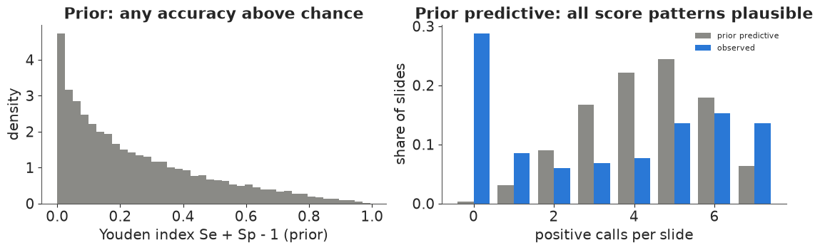
The prior allows anything from useless to perfect raters, but the Youden index leans toward small values, and the prior predictive shows what that means: raters this mediocre would almost never be unanimous (under 1% of slides with 0 calls, 6% with 7), while 42% of the real slides are unanimous. "Uniform on accuracy" is not "uninformative about agreement". We keep it anyway, for two reasons: with 118 slides spread over 127 pattern cells the data overwhelm it, and it lets us compare with maximum likelihood below. With fewer items, a prior that expects competent raters (say fpr ~ Beta(1, 4) and u ~ Beta(3, 1)) would be the better choice. Now fit, nutpie defaults.
t0 = time.time()
with lcm2(Y) as m_ci:
    idata_ci = pm.sample(random_seed=RANDOM_SEED, progressbar=False)
print(f"{time.time() - t0:.0f} s, tuning steps {idata_ci.posterior.attrs.get('tuning_steps')}; "
      f"{diag(idata_ci, ['pi', 'se', 'sp'])}")


def rater_table(idata, cols=("se", "sp")):
    out = {}
    for c in cols:
        x = draws(idata, c)
        out[c] = [f"{np.mean(x[:, j]):.2f} [{np.quantile(x[:, j], 0.05):.2f}, "
                  f"{np.quantile(x[:, j], 0.95):.2f}]" for j in range(x.shape[1])]
    return pd.DataFrame(out, index=RATERS)


print(f"prevalence pi: mean {draws(idata_ci, 'pi').mean():.3f}, 90% {q(draws(idata_ci, 'pi'))[[0, 2]]}")
rater_table(idata_ci)
2 s, tuning steps 400; divergences 0, max r_hat 1.003, min bulk ESS 1742
prevalence pi: mean 0.526, 90% [0.442 0.609]
| se | sp | |
|---|---|---|
| A | 0.95 [0.88, 1.00] | 0.87 [0.79, 0.94] |
| B | 0.97 [0.93, 0.99] | 0.67 [0.55, 0.78] |
| C | 0.72 [0.61, 0.82] | 0.98 [0.95, 1.00] |
| D | 0.52 [0.41, 0.63] | 0.98 [0.95, 1.00] |
| E | 0.96 [0.91, 0.99] | 0.80 [0.70, 0.89] |
| F | 0.41 [0.31, 0.51] | 0.98 [0.95, 1.00] |
| G | 0.98 [0.93, 1.00] | 0.91 [0.82, 0.98] |
Check against maximum likelihood. Agresti (2002) and the poLCA documentation report a maximised log-likelihood of $-317.2568$ for this model. A few lines of EM (the algorithm Dawid & Skene introduced for exactly this problem) reproduce it:
def em_lcm2(Y_, iters=3000):
    pi_, se_, fp_ = 0.5, np.full(Y_.shape[1], 0.8), np.full(Y_.shape[1], 0.2)
    for _ in range(iters):
        l1 = np.log(pi_) + (Y_ * np.log(se_) + (1 - Y_) * np.log1p(-se_)).sum(axis=1)
        l0 = np.log1p(-pi_) + (Y_ * np.log(fp_) + (1 - Y_) * np.log1p(-fp_)).sum(axis=1)
        ll = np.logaddexp(l1, l0)
        w = np.exp(l1 - ll)                                       # E-step: P(D = 1 | y)
        pi_ = w.mean()                                            # M-step
        se_ = np.clip((w[:, None] * Y_).sum(axis=0) / w.sum(), 1e-12, 1 - 1e-12)
        fp_ = np.clip(((1 - w)[:, None] * Y_).sum(axis=0) / (1 - w).sum(), 1e-12, 1 - 1e-12)
    return pi_, se_, 1 - fp_, ll.sum()


pi_em, se_em, sp_em, ll_em = em_lcm2(Y)
print(f"EM log-likelihood {ll_em:.4f}, prevalence {pi_em:.3f}")
print(pd.DataFrame({"Se (EM)": se_em, "Sp (EM)": sp_em,
                    "Se (posterior mean)": draws(idata_ci, "se").mean(axis=0),
                    "Sp (posterior mean)": draws(idata_ci, "sp").mean(axis=0)}, index=RATERS).round(3).T)
EM log-likelihood -317.2568, prevalence 0.501
                         A      B      C      D      E      F      G
Se (EM)              1.000  0.983  0.761  0.541  0.979  0.423  1.000
Sp (EM)              0.883  0.646  1.000  1.000  0.777  1.000  0.883
Se (posterior mean)  0.950  0.969  0.719  0.517  0.961  0.406  0.977
Sp (posterior mean)  0.874  0.670  0.982  0.982  0.799  0.983  0.907
The log-likelihood matches to four decimals. The maximum likelihood estimates put three sensitivities (A, G, nearly B) and three specificities (C, D, F) exactly on the boundary: "pathologist A never misses a carcinoma" from 118 slides. The posterior means are pulled inside (0.95 instead of 1.00), with intervals that say how far the data allow: a 90% lower bound of about 0.88 for A's sensitivity. That is the practical value of the Bayesian fit here: honest uncertainty where maximum likelihood gives a corner.
The model's picture is clear and plausible: two styles of pathologist. A, B, E, G rarely miss (sensitivity 0.95 or more) but over-call (specificity 0.67-0.91); C, D, F almost never over-call but miss 28-59% of carcinomas. Prevalence about 0.53.
4 · Is conditional independence believable?
Conditional independence says that, once the true status is known, one pathologist's call tells you nothing about another's. For slides that are genuinely borderline this is implausible: a hard slide is hard for everyone. The model is fitted to the whole pattern table, but two summaries are sensitive to exactly this failure:
- the distribution of the number of positive calls per slide (0-7); dependence among raters within a class piles slides into the middle scores the model cannot produce;
- the pairwise agreement of every pair of raters (21 pairs).
We replicate the 118 slides from the posterior (new true statuses, new calls) and compare.
def replicate_lc(pi_or_w, rates, n_rep=1000, seed=0):
    """Generic latent class simulator: class weights (S, C) and positive rates (S, J, C)."""
    g = np.random.default_rng(seed)
    idx = g.choice(len(rates), n_rep, replace=False)
    w, r = pi_or_w[idx], rates[idx]
    cls = (g.random((n_rep, N, 1)) > np.cumsum(w, axis=1)[:, None, :]).sum(axis=2)  # (rep, N)
    p = np.take_along_axis(r[:, None, :, :], cls[:, :, None, None], axis=3)[..., 0]  # (rep, N, J)
    return (g.random(p.shape) < p).astype(int)


def score_hist(Yr):
    return np.stack([(Yr.sum(axis=-1) == k).sum(axis=-1) for k in range(J + 1)], axis=-1)


def pair_agree(Yr):
    return np.stack([(Yr[..., a] == Yr[..., b]).mean(axis=-1) for a, b in pairs], axis=-1)


pi_d = draws(idata_ci, "pi")
w_ci = np.stack([1 - pi_d, pi_d], axis=1)
rates_ci = np.stack([1 - draws(idata_ci, "sp"), draws(idata_ci, "se")], axis=2)
yrep_ci = replicate_lc(w_ci, rates_ci)
obs_score, obs_agree = score_hist(Y), pair_agree(Y)


def ppc_summary(yrep, label):
    sh, ag = score_hist(yrep), pair_agree(yrep)
    z = (obs_agree - ag.mean(axis=0)) / ag.std(axis=0)
    p_hi = (sh >= obs_score).mean(axis=0)
    print(f"{label}: observed vs replicated (mean) slides by score")
    print(pd.DataFrame({"observed": obs_score, "replicated": sh.mean(axis=0).round(1),
                        "P(rep >= obs)": p_hi.round(3)}, index=range(J + 1)).T)
    print(f"  pairwise agreement z-scores: min {z.min():.2f}, max {z.max():.2f}; "
          f"pairs with |z| > 2: {int((np.abs(z) > 2).sum())} of {len(pairs)}")
    return sh, z


sh_ci, z_ci = ppc_summary(yrep_ci, "conditional independence")
conditional independence: observed vs replicated (mean) slides by score
                    0       1      2      3      4     5       6       7
observed       34.000  10.000  7.000  8.000  9.000  16.0  18.000  16.000
replicated     22.500  23.100  8.500  2.200  7.500  22.3  23.800   8.100
P(rep >= obs)   0.043   0.995  0.682  0.012  0.378   0.9   0.902   0.025
  pairwise agreement z-scores: min 0.17, max 2.51; pairs with |z| > 2: 2 of 21
The failure is in the middle of the score distribution. The model expects about 23 slides with exactly one positive call and 2 with exactly three; the data have 10 and 8 (posterior predictive probabilities 0.995 and 0.012). It also expects too few unanimous slides at both ends (22 vs 34 with no positive call, 8 vs 16 with seven). The pairwise agreements lean the same way: every pair agrees more often than the model predicts (z from 0.2 to 2.5), which is what errors shared between raters look like. The pattern is the signature of conditional dependence: slides that fool one pathologist tend to fool several, so "3 of 7" is more common than independent errors allow, and "1 of 7" (one idiosyncratic error) less.
Why this matters: under conditional independence the model reads agreement between raters as evidence that they are all accurate. If part of that agreement is shared confusion, accuracy (and our certainty about the true labels) is overstated.
5 · Two ways to model the dependence
5.1 · Random effects: a latent "difficulty" per slide
Qu, Tan & Kutner (1996) gave each item a continuous random effect $b_i \sim \mathcal N(0, 1)$ that shifts every rater's probability of a positive call within a class:
$$P(y_{ij} = 1 \mid D_i = d, b_i) = \operatorname{logit}^{-1}(a_{jd} + s\, b_i).$$
(They used a probit link and allowed a different $s$ per class; we use a logit and one shared
$s$.) Now there are two latent quantities per slide. The discrete $D_i$ is summed out as before;
the continuous $b_i$ is integrated out by Gauss-Hermite quadrature with 20 nodes, all
inside one logsumexp. Sensitivity and specificity become averages over slides:
$\mathrm{Se}_j = \int \operatorname{logit}^{-1}(a_{j1} + s b)\,\phi(b)\,db$. The "better than
chance" constraint is $a_{j1} = a_{j0} + \delta_j$ with $\delta_j > 0$.
GH_X, GH_W = np.polynomial.hermite_e.hermegauss(20)       # nodes/weights for exp(-x^2/2)
GH_W = GH_W / np.sqrt(2 * np.pi)                           # now a quadrature for N(0, 1)
print(f"Gauss-Hermite check: E[b^2] = {GH_W @ GH_X**2:.6f}, E[logistic(1 + 2b)] = "
      f"{GH_W @ special.expit(1 + 2 * GH_X):.5f} vs Monte Carlo "
      f"{special.expit(1 + 2 * np.random.default_rng(0).standard_normal(10**6)).mean():.5f}")


def log_bern_sum(eta):
    """eta (nodes, J) -> (N, nodes): sum_j log P(y_ij | eta)."""
    lp = (Y[:, None, :] * (-pt.softplus(-eta))[None] + (1 - Y[:, None, :]) * (-pt.softplus(eta))[None])
    return lp.sum(axis=-1)


with pm.Model(coords={"rater": RATERS, "item": np.arange(N)}) as m_re:
    pi = pm.Beta("pi", 1.0, 1.0)
    a0 = pm.Normal("a0", -2.0, 1.5, dims="rater")
    delta = pm.HalfNormal("delta", 4.0, dims="rater")
    a1 = pm.Deterministic("a1", a0 + delta, dims="rater")
    s = pm.HalfNormal("s", 1.5)
    eta0 = a0[None, :] + s * GH_X[:, None]                  # (nodes, rater)
    eta1 = a1[None, :] + s * GH_X[:, None]
    l1 = pt.log(pi) + pt.logsumexp(np.log(GH_W)[None] + log_bern_sum(eta1), axis=1)
    l0 = pt.log1p(-pi) + pt.logsumexp(np.log(GH_W)[None] + log_bern_sum(eta0), axis=1)
    ll = pt.logaddexp(l1, l0)
    pm.Potential("lik", ll.sum())
    pm.Deterministic("ll", ll, dims="item")
    pm.Deterministic("p_pos", pt.exp(l1 - ll), dims="item")
    pm.Deterministic("se", GH_W @ pt.sigmoid(eta1), dims="rater")
    pm.Deterministic("sp", 1 - GH_W @ pt.sigmoid(eta0), dims="rater")

t0 = time.time()
with m_re:
    idata_re = pm.sample(random_seed=RANDOM_SEED, progressbar=False)
print(f"{time.time() - t0:.0f} s; {diag(idata_re, ['pi', 'a0', 'delta', 's'])}")
print(f"s (random-effect sd, logit scale): {q(draws(idata_re, 's'))}; "
      f"prevalence: {q(draws(idata_re, 'pi'))}")
rater_table(idata_re)
Gauss-Hermite check: E[b^2] = 1.000000, E[logistic(1 + 2b)] = 0.64773 vs Monte Carlo 0.64797
4 s; divergences 0, max r_hat 1.004, min bulk ESS 794
s (random-effect sd, logit scale): [3.392 4.26  5.143]; prevalence: [0.223 0.516 0.878]
| se | sp | |
|---|---|---|
| A | 0.70 [0.56, 0.90] | 0.58 [0.47, 0.71] |
| B | 0.84 [0.71, 0.97] | 0.50 [0.38, 0.65] |
| C | 0.52 [0.37, 0.73] | 0.78 [0.67, 0.87] |
| D | 0.32 [0.23, 0.44] | 0.78 [0.71, 0.87] |
| E | 0.79 [0.63, 0.95] | 0.59 [0.46, 0.73] |
| F | 0.25 [0.18, 0.36] | 0.82 [0.76, 0.89] |
| G | 0.73 [0.58, 0.90] | 0.62 [0.51, 0.74] |
g = np.random.default_rng(1)
idx = g.choice(len(draws(idata_re, "pi")), 1000, replace=False)
pi_r, a0_r, a1_r, s_r = (draws(idata_re, v)[idx] for v in ["pi", "a0", "a1", "s"])
D_r = g.random((1000, N)) < pi_r[:, None]
b_r = g.standard_normal((1000, N))
eta_r = np.where(D_r[..., None], a1_r[:, None, :], a0_r[:, None, :]) + (s_r[:, None] * b_r)[..., None]
yrep_re = (g.random(eta_r.shape) < special.expit(eta_r)).astype(int)
sh_re, z_re = ppc_summary(yrep_re, "random effects")
random effects: observed vs replicated (mean) slides by score
                    0       1       2      3       4       5       6       7
observed       34.000  10.000   7.000   8.00   9.000  16.000  18.000  16.000
replicated     28.100  12.100  10.100  10.90  13.200  14.200  11.800  17.600
P(rep >= obs)   0.181   0.758   0.874   0.85   0.896   0.351   0.064   0.627
  pairwise agreement z-scores: min -0.50, max 1.91; pairs with |z| > 2: 0 of 21
The random-effects model reproduces the score distribution (every posterior predictive probability between 0.06 and 0.9) and the pairwise agreements (no |z| > 2). By this check it is a much better model. But look at what it says about the pathologists and the slides:
- the random-effect sd is about 4 on the logit scale - larger than the gaps between the classes for most pathologists;
- the prevalence is anywhere from about 0.2 to 0.9;
- sensitivities have collapsed to 0.25-0.84 and specificities to 0.50-0.82.
The continuous slide effect has taken over the job of the class. The picture is clearest in the probability each model gives that a slide has carcinoma, as a function of how many pathologists said so:
def p_by_score(idata):
    p = idata.posterior["p_pos"].mean(("chain", "draw")).to_numpy()
    return p


fig, ax = plt.subplots(figsize=(9, 4))
jit = np.random.default_rng(2).uniform(-0.12, 0.12, N)
ax.scatter(k_pos + jit - 0.15, p_by_score(idata_ci), s=16, color=BLUE, alpha=0.7,
           label="conditional independence")
ax.scatter(k_pos + jit + 0.15, p_by_score(idata_re), s=16, color=RED, alpha=0.7,
           label="random effects (shared s)")
ax.set(xlabel="number of pathologists (of 7) calling carcinoma", ylabel="P(carcinoma | calls)",
       title="The random-effects model fits better, and no longer knows which slides have carcinoma")
ax.legend(fontsize=8, loc="center right");
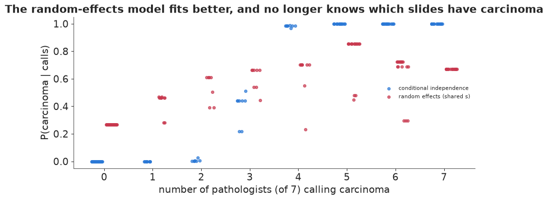
Under conditional independence the probability of carcinoma climbs from 0 to 1 as more pathologists say yes, crossing 1/2 at three or four calls. Under the random-effects model a slide on which all seven pathologists see nothing has about a 27% chance of carcinoma, and a slide on which all seven see carcinoma only about 67%, less than some slides with five calls. The model is not wrong about the data; it has found a different explanation for them: slides vary along a continuous "looks malignant" scale, and the two classes are no longer tied to the pathologists' calls in any strong way.
This is Albert & Dodd's (2004) warning: different conditional-dependence structures can fit the observed patterns equally well and still give very different sensitivities, specificities and prevalence, because with no gold standard the class is defined only through the model. A better fit is not a better answer if the latent class stopped meaning "carcinoma".
5.2 · A third class: slides that are genuinely ambiguous
Agresti (2002, p. 543) fits a three-class model to these data (maximised log-likelihood -293.7 against -317.3 for two classes, as reproduced in the poLCA documentation). The interpretation is direct: there are clearly negative slides, clearly positive slides, and a group of borderline slides on which each pathologist's call depends on his or her threshold. We check it with the same predictive tools. Conditional independence is then assumed within each of the three classes.
The label-switching fix generalises: for each pathologist the probability of a positive call
must increase from class "negative" to "ambiguous" to "positive". We sample the logits
$a_{j,\cdot}$ with the ordered transform along the class axis.
CLS = ["negative", "ambiguous", "positive"]
with pm.Model(coords={"rater": RATERS, "item": np.arange(N), "cls": CLS}) as m_lc3:
    w = pm.Dirichlet("w", np.ones(3), dims="cls")
    a = pm.Normal("a", np.array([-2.5, 0.0, 2.5]), 2.0, dims=("rater", "cls"),
                  transform=pm.distributions.transforms.ordered)
    lp = (Y[:, :, None] * (-pt.softplus(-a))[None]
          + (1 - Y[:, :, None]) * (-pt.softplus(a))[None]).sum(axis=1)       # (item, cls)
    lj = pt.log(w)[None] + lp
    ll = pt.logsumexp(lj, axis=1)
    pm.Potential("lik", ll.sum())
    pm.Deterministic("ll", ll, dims="item")
    pm.Deterministic("p_cls", pt.exp(lj - ll[:, None]), dims=("item", "cls"))
    pm.Deterministic("p_pos", pt.exp(lj[:, 2] - ll), dims="item")
    pm.Deterministic("rate", pt.sigmoid(a), dims=("rater", "cls"))

t0 = time.time()
with m_lc3:
    idata_lc3 = pm.sample(random_seed=RANDOM_SEED, progressbar=False,
                          initvals={"a": np.tile([-2.0, 0.0, 2.0], (J, 1))})
print(f"{time.time() - t0:.0f} s; {diag(idata_lc3, ['w', 'a'])}")
print("class weights:", {c: q(draws(idata_lc3, "w")[:, k]).tolist() for k, c in enumerate(CLS)})
# az.summary on a 2-D variable can mislabel rows: tabulate from the arrays directly
rate_d = draws(idata_lc3, "rate")                                            # (S, rater, cls)
print("P(positive call | class), posterior mean:")
print(pd.DataFrame(rate_d.mean(axis=0), index=RATERS, columns=CLS).round(2).T)
3 s; divergences 0, max r_hat 1.006, min bulk ESS 1758
class weights: {'negative': [0.291, 0.372, 0.456], 'ambiguous': [0.12, 0.191, 0.274], 'positive': [0.346, 0.435, 0.521]}
P(positive call | class), posterior mean:
              A     B     C     D     E     F     G
negative   0.06  0.14  0.01  0.01  0.06  0.01  0.02
ambiguous  0.52  0.92  0.08  0.09  0.76  0.06  0.64
positive   0.99  0.98  0.85  0.61  0.98  0.49  0.99
rates_lc3 = rate_d
yrep_lc3 = replicate_lc(draws(idata_lc3, "w"), rates_lc3)
sh_lc3, z_lc3 = ppc_summary(yrep_lc3, "three classes")
for idt in [idata_ci, idata_re, idata_lc3]:
idt["log_likelihood"] = xr.Dataset({"y": idt.posterior["ll"]})
loo = {name: az.loo(idt, var_name="y", pointwise=True)
for name, idt in [("2 classes, independent", idata_ci), ("2 classes + random effect", idata_re),
("3 classes, independent", idata_lc3)]}
print("max Pareto k:", {k: round(float(v.pareto_k.max()), 2) for k, v in loo.items()})
az.compare(loo, round_to=1)
three classes: observed vs replicated (mean) slides by score
                    0       1      2     3      4       5       6       7
observed       34.000  10.000  7.000  8.00  9.000  16.000  18.000  16.000
replicated     31.500  12.200  6.600  8.90  8.500  14.500  23.600  12.300
P(rep >= obs)   0.366   0.701  0.482  0.64  0.451   0.373   0.875   0.211
  pairwise agreement z-scores: min -0.25, max 1.81; pairs with |z| > 2: 0 of 21
max Pareto k: {'2 classes, independent': 0.53, '2 classes + random effect': 0.21, '3 classes, independent': 0.48}| rank | elpd_diff | dse | p_worse | diag_diff | diag_elpd | p | elpd | se | weight | |
|---|---|---|---|---|---|---|---|---|---|---|
| 2 classes + random effect | 0 | 0.0 | 0.0 | NaN | 9.1 | -312.1 | 12.5 | 0.6 | ||
| 3 classes, independent | 1 | -2.0 | 4.1 | 0.7 | |elpd_diff| < 4 | 13.1 | -314.1 | 13.1 | 0.4 | |
| 2 classes, independent | 2 | -20.7 | 7.9 | 1.0 | 10.8 | -332.8 | 13.0 | 0.0 |
The three-class model passes the same score check as the random-effects model and has essentially the same expected predictive accuracy (the difference is about 2 nats with a standard error of about 4); both beat conditional independence by about 20 nats (leaving one slide out at a time, which is the unit a new slide would be).
The two good models differ in what they say about each slide. The figure puts the three models side by side: the score check, and the probability of carcinoma per slide.
fig, axes = plt.subplots(1, 3, figsize=(16, 4.2), width_ratios=[1.2, 1.2, 1])
for k, (sh, col, lab) in enumerate([(sh_ci, BLUE, "2 classes"), (sh_re, RED, "random effects"),
                                    (sh_lc3, AQUA, "3 classes")]):
    lo, hi = np.quantile(sh, [0.05, 0.95], axis=0)
    xs = np.arange(J + 1) + (k - 1) * 0.22
    axes[0].vlines(xs, lo, hi, color=col, lw=4, alpha=0.7, label=f"{lab} (90% of replications)")
axes[0].scatter(np.arange(J + 1), obs_score, color="k", zorder=3, s=25, label="observed")
axes[0].set(xlabel="positive calls per slide", ylabel="slides", title="Score check")
axes[0].legend(fontsize=7)
pc = idata_lc3.posterior["p_cls"].mean(("chain", "draw")).to_numpy()
axes[1].scatter(k_pos + jit - 0.15, pc[:, 2], s=16, color=AQUA, label="P(positive class)")
axes[1].scatter(k_pos + jit + 0.15, pc[:, 1], s=16, color=ORANGE, label="P(ambiguous class)")
axes[1].scatter(k_pos + jit, p_by_score(idata_ci), s=10, color=BLUE, marker="x", alpha=0.6,
                label="P(carcinoma), 2 classes")
axes[1].set(xlabel="positive calls (of 7)", ylabel="posterior probability",
            title="Three classes: the middle scores are 'ambiguous'")
axes[1].legend(fontsize=7)
for j in range(J):
    lo, mid, hi = np.quantile(rate_d[:, j, :], [0.05, 0.5, 0.95], axis=0)
    axes[2].errorbar(np.arange(3) + (j - 3) * 0.08, mid, yerr=[mid - lo, hi - mid], marker="o",
                     ms=3, lw=1, capsize=0, label=RATERS[j])
axes[2].set_xticks(range(3), CLS)
axes[2].set(ylabel="P(pathologist calls carcinoma)", title="Each pathologist's threshold")
axes[2].legend(fontsize=7, ncol=2);
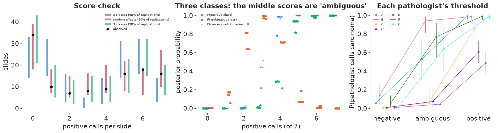
The three-class model keeps the meaning of the classes: slides with 0-1 positive calls are negative, slides with 5-7 are positive, and slides with 2-4 positive calls are mostly ambiguous. The right panel shows why pathologists disagree so much: on clearly negative and clearly positive slides they nearly all agree (except that D and F still miss a fair share of the positive class), and on ambiguous slides their calls spread from about 0.06 (F) to over 0.9 (B): the disagreement is a difference in thresholds on hard slides, not random error.
What is the "sensitivity" of pathologist F? It depends on whether an ambiguous slide counts as carcinoma - a clinical definition, not something the data can settle. The model makes the question explicit instead of hiding it.
6 · When can the data answer at all?
6.1 · Counting parameters and degrees of freedom
A latent class model is only identifiable if the pattern table has at least as many free cells as the model has parameters (necessary, not sufficient):
rows = []
for R_ in range(1, 8):
    rows.append({"raters": R_, "df = 2^R - 1": 2**R_ - 1, "2 classes: 2R + 1": 2 * R_ + 1,
                 "3 classes: 3R + 2": 3 * R_ + 2, "2 classes + RE: 2R + 2": 2 * R_ + 2})
ident = pd.DataFrame(rows).set_index("raters")
ident
| df = 2^R - 1 | 2 classes: 2R + 1 | 3 classes: 3R + 2 | 2 classes + RE: 2R + 2 | |
|---|---|---|---|---|
| raters | ||||
| 1 | 1 | 3 | 5 | 4 |
| 2 | 3 | 5 | 8 | 6 |
| 3 | 7 | 7 | 11 | 8 |
| 4 | 15 | 9 | 14 | 10 |
| 5 | 31 | 11 | 17 | 12 |
| 6 | 63 | 13 | 20 | 14 |
| 7 | 127 | 15 | 23 | 16 |
With two raters the two-class model has 5 parameters and the data 3 degrees of freedom: no amount of data identifies the prevalence or the accuracies. Three raters are just identified; three classes need four raters (15 >= 14), and so does the random-effects model (15 >= 10).
Hui & Walter (1980) found the classic escape for two tests: apply them in two populations with different prevalence, assuming each test's sensitivity and specificity are the same in both. Then there are $2 \times 3 = 6$ degrees of freedom and $2 + 2 + 2 = 6$ parameters. Just identified - if the prevalences differ. We test this on simulated data where the truth is known.
6.2 · Hui-Walter, simulated
Two tests with Se = (0.90, 0.75) and Sp = (0.95, 0.98), 400 subjects per population. Scenario 1: prevalences 0.15 and 0.50. Scenario 2: both 0.30.
SE_T, SP_T, NG = np.array([0.90, 0.75]), np.array([0.95, 0.98]), 400


def simulate_hw(prevs, seed):
    g = np.random.default_rng(seed)
    grp = np.repeat(np.arange(2), NG)
    Dh = g.random(2 * NG) < np.asarray(prevs)[grp]
    Yh = (g.random((2 * NG, 2)) < np.where(Dh[:, None], SE_T, 1 - SP_T)).astype(int)
    return grp, Yh


def hui_walter(grp, Yh):
    with pm.Model(coords={"test": ["test 1", "test 2"], "pop": ["pop 1", "pop 2"]}) as m:
        prev = pm.Beta("prev", 1.0, 1.0, dims="pop")
        fpr = pm.Beta("fpr", 1.0, 1.0, dims="test")
        se = pm.Deterministic("se", fpr + (1 - fpr) * pm.Beta("u", 1.0, 1.0, dims="test"), dims="test")
        pm.Deterministic("sp", 1 - fpr, dims="test")
        l1 = pt.log(prev[grp]) + (Yh * pt.log(se) + (1 - Yh) * pt.log1p(-se)).sum(axis=1)
        l0 = pt.log1p(-prev[grp]) + (Yh * pt.log(fpr) + (1 - Yh) * pt.log1p(-fpr)).sum(axis=1)
        pm.Potential("lik", pt.logaddexp(l1, l0).sum())
    return m


hw = {}
for label, prevs in [("prevalences 0.15 / 0.50", (0.15, 0.50)), ("prevalences 0.30 / 0.30", (0.30, 0.30))]:
    with hui_walter(*simulate_hw(prevs, seed=5)):
        hw[label] = pm.sample(random_seed=RANDOM_SEED, progressbar=False, target_accept=0.95)
    print(f"{label}: {diag(hw[label], ['prev', 'se', 'sp'])}")
    print(f"   Se test 1 90%: {q(draws(hw[label], 'se')[:, 0])[[0, 2]]} (truth 0.90); "
          f"Se test 2: {q(draws(hw[label], 'se')[:, 1])[[0, 2]]} (0.75); "
          f"prevalence pop 1: {q(draws(hw[label], 'prev')[:, 0])[[0, 2]]}")
prevalences 0.15 / 0.50: divergences 0, max r_hat 1.005, min bulk ESS 1168
   Se test 1 90%: [0.87  0.967] (truth 0.90); Se test 2: [0.744 0.871] (0.75); prevalence pop 1: [0.115 0.195]
prevalences 0.30 / 0.30: divergences 0, max r_hat 1.003, min bulk ESS 783
   Se test 1 90%: [0.823 0.992] (truth 0.90); Se test 2: [0.717 0.983] (0.75); prevalence pop 1: [0.218 0.361]
fig, axes = plt.subplots(1, 3, figsize=(15, 4))
for (label, idt), col in zip(hw.items(), [BLUE, ORANGE]):
    se1, se2, pv = draws(idt, "se")[:, 0], draws(idt, "se")[:, 1], draws(idt, "prev")[:, 0]
    axes[0].scatter(se1, se2, s=3, alpha=0.2, color=col, label=label)
    axes[1].scatter(se1, pv, s=3, alpha=0.2, color=col)
    axes[2].hist(draws(idt, "sp")[:, 1], bins=np.linspace(0.85, 1, 50), alpha=0.6, color=col,
                 density=True)
axes[0].scatter([SE_T[0]], [SE_T[1]], marker="*", s=200, color="k", label="truth")
axes[1].scatter([SE_T[0]], [0.15], marker="*", s=200, color="k")
axes[1].scatter([SE_T[0]], [0.30], marker="*", s=200, color="k")
axes[2].axvline(SP_T[1], color="k", ls="--", label="truth")
axes[0].set(xlabel="Se of test 1", ylabel="Se of test 2", xlim=(0.6, 1), ylim=(0.5, 1),
            title="Sensitivities")
axes[1].set(xlabel="Se of test 1", ylabel="prevalence in population 1", xlim=(0.6, 1),
            title="Sensitivity trades off against prevalence")
axes[2].set(xlabel="Sp of test 2", ylabel="density", title="Specificity of test 2")
from matplotlib.lines import Line2D
axes[0].legend(handles=[Line2D([], [], ls="", marker="o", color=c, label=l) for c, l in
                        zip([BLUE, ORANGE], hw)] + [Line2D([], [], ls="", marker="*", ms=12,
                                                           color="k", label="truth")], fontsize=8)
axes[2].legend(fontsize=8);
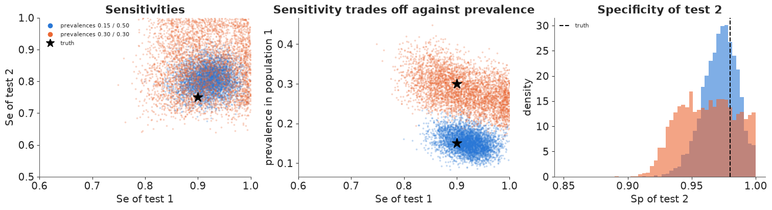
With different prevalences the posterior concentrates around the truth (Se of test 1: 90% interval 0.87-0.97; the prevalence of population 1: 0.12-0.20 around a true 0.15). With equal prevalences the two populations are one population, the model has 5 parameters for 3 degrees of freedom, and the posterior is much wider, piles up against Se = 1 and Sp = 1, and trades sensitivity against prevalence (middle panel). It does not spread over everything: the "better than chance" constraint and the 0-1 bounds confine it - partial identification. The sampler reports no problem in either case: diagnostics check the computation, not whether the question was answerable. (Hui-Walter's assumption that accuracy is the same in both populations is itself untestable in the just-identified design; with a third test or population it becomes checkable.)
6.3 · Two pathologists: what informative priors buy
Back to real data. Suppose only pathologists A and C had read the slides. Two raters, 3 degrees of freedom, 5 parameters: two equations short. What do we learn about the prevalence of carcinoma?
- (a) with the vague "better than chance" priors used so far;
- (b) with two informative priors, A's sensitivity ~ Beta(38, 2) (mean 0.95) and C's specificity ~ Beta(49, 1) (mean 0.98), as a lab might have from validation studies;
- (c) with two informative priors on one pathologist, A's sensitivity ~ Beta(38, 2) and A's specificity ~ Beta(35, 5) (mean 0.875).
The values are illustrative, chosen close to what the seven-rater model says about A and C, so that we can see whether the two-rater analysis gets back to the seven-rater answer.
sub = [RATERS.index("A"), RATERS.index("C")]
two = {}
for label, kw in [("(a) vague", {}),
                  ("(b) Se of A + Sp of C", {"youden": False, "se_prior": {0: (38.0, 2.0)},
                                             "sp_prior": {1: (49.0, 1.0)}}),
                  ("(c) Se and Sp of A", {"youden": False, "se_prior": {0: (38.0, 2.0)},
                                          "sp_prior": {0: (35.0, 5.0)}})]:
    with lcm2(Y[:, sub], **kw):
        two[label] = pm.sample(random_seed=RANDOM_SEED, progressbar=False, target_accept=0.95)
    print(f"A + C only, {label}: {diag(two[label], ['pi', 'se', 'sp'])}; "
          f"prevalence mean {draws(two[label], 'pi').mean():.2f}, 90% {q(draws(two[label], 'pi'))[[0, 2]]}")
print(f"all seven, 2-class model: prevalence 90% {q(draws(idata_ci, 'pi'))[[0, 2]]}")
print(f"observed: A calls {Y[:, sub[0]].mean():.2f} of slides positive, C {Y[:, sub[1]].mean():.2f}; "
      f"C positive but A negative on {np.mean((Y[:, sub[1]] == 1) & (Y[:, sub[0]] == 0)):.3f}")

fig, ax = plt.subplots(figsize=(9, 3.6))
bins = np.linspace(0, 1, 80)
ax.hist(np.random.default_rng(0).beta(1, 1, 4000), bins=bins, density=True, histtype="step",
        color=GREY, lw=1.5, label="prior")
for (label, idt), col in zip(two.items(), [ORANGE, PURPLE, RED]):
    ax.hist(draws(idt, "pi"), bins=bins, density=True, histtype="step", lw=2, color=col,
            label=f"A + C, {label}")
ax.hist(draws(idata_ci, "pi"), bins=bins, density=True, alpha=0.35, color=BLUE, label="all 7 raters")
ax.set(xlabel="prevalence of carcinoma", ylabel="density",
       title="Two raters: which priors can stand in for the missing data?")
ax.legend(fontsize=8);
A + C only, (a) vague: divergences 0, max r_hat 1.011, min bulk ESS 712; prevalence mean 0.47, 90% [0.354 0.585]
A + C only, (b) Se of A + Sp of C: divergences 0, max r_hat 1.005, min bulk ESS 810; prevalence mean 0.47, 90% [0.356 0.59 ]
A + C only, (c) Se and Sp of A: divergences 0, max r_hat 1.002, min bulk ESS 1801; prevalence mean 0.50, 90% [0.397 0.591]
all seven, 2-class model: prevalence 90% [0.442 0.609]
observed: A calls 0.56 of slides positive, C 0.38; C positive but A negative on 0.000
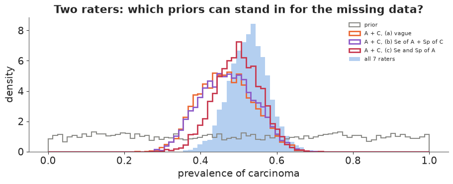
Three lessons, none of which a sampler diagnostic would reveal (all three fits are clean):
- Vague priors do not give "anything goes". The prevalence is confined to roughly 0.35-0.59. This is partial identification: C never calls a slide positive that A calls negative, and if both are better than chance the prevalence lies roughly between C's positive rate (0.38, reached if C is perfectly specific) and A's (0.56, if A is perfectly sensitive). The data identify the bounds; where the posterior sits between them comes from the prior.
- An informative prior helps only if it bears on the unidentified direction. Priors saying that A is very sensitive and C very specific (b) change nothing: they merely confirm that the edges of the bounds are plausible.
- Priors on both accuracies of one rater (c) pin the prevalence through $\pi = (P(A+) - \mathrm{fpr}_A)/(\mathrm{Se}_A - \mathrm{fpr}_A)$ and shift it toward the seven-rater answer (mean 0.50 vs 0.47 with vague priors; 0.53 with all seven raters), cutting off the low end of the bounds (5% quantile 0.40 vs 0.35). What width remains comes from 118 slides and from the prior's own width. The narrowing is the prior's doing: a different validation study would give a different answer from the same data, and it must be reported as an assumption, not a finding.
7 · More than two categories: Dawid & Skene's anaesthetists
7.1 · Data
Dawid & Skene (1979) introduced the EM algorithm for this problem with 45 patients whose fitness for anaesthesia five anaesthetists rated on a 4-point scale from a standard form. Anaesthetist 1 rated every form three times, weeks apart.
data.describe("anesthesia_dawid_skene")
an = data.load("anesthesia_dawid_skene")
item, rater, lab = an["item"].to_numpy() - 1, an["rater"].to_numpy() - 1, an["rating"].to_numpy() - 1
I_A, J_A, K_A = item.max() + 1, rater.max() + 1, 4
counts = np.zeros((I_A, K_A))
np.add.at(counts, (item, lab), 1)                        # votes per patient and category
print(pd.crosstab(an.rater, an.rating, margins=True))
r1 = np.stack([lab[(item == i) & (rater == 0)] for i in range(I_A)])   # anaesthetist 1, 3 readings
print(f"anaesthetist 1 gave the same rating on all three readings for {np.mean(r1.min(1) == r1.max(1)):.0%} "
      f"of patients")
mv_a = counts.argmax(axis=1)
ties = (counts == counts.max(axis=1, keepdims=True)).sum(axis=1) > 1
print(f"majority vote (7 ratings per patient): ties for patients {(np.where(ties)[0] + 1).tolist()}")
anesthesia_dawid_skene: Pre-operative assessments of 45 patients by 5 anaesthetists on a 4-point ordinal scale of pre-operative health, made from a standard form; anaesthetist 1 assessed every form three times weeks apart, the others once (315 ratings). Long format: item (patient, 1-45), rater (1-5), rating (1-4).
  source: Dawid & Skene (1979), Applied Statistics 28:20-28, Table 1; distributed as `anesthesia` in the CRAN package rater (Pullin, Gurrin & Vukcevic; GPL-2; the URL). CONVERTED from the .rda with R - keep the CSV in data/. An independent transcription (github.com/dallascard/dawid_skene) differs in one reading (patient 7, anaesthetist 1: 1,1,2 here vs 1,2,2).
  url:    https://raw.githubusercontent.com/cran/rater/master/data/anesthesia.rda
rating    1    2   3   4  All
rater
1        53   60  18   4  135
2        16   15  11   3   45
3        20   17   5   3   45
4        18   17   7   3   45
5        21   15   7   2   45
All     128  124  48  15  315
anaesthetist 1 gave the same rating on all three readings for 71% of patients
majority vote (7 ratings per patient): ties for patients [12]
Category 4 is rare (15 of 315 ratings), and anaesthetist 1 disagrees with himself on 29% of the patients - repeated reading is a rater effect of its own.
7.2 · The Dawid-Skene model with pooled confusion matrices
Each rater $j$ has a confusion matrix $\theta_j$: row $k$ is the distribution of the rating the rater gives to a patient whose true category is $k$. Given the true category, ratings are independent (including anaesthetist 1's three readings, an assumption we check below). The true category is summed out:
$$p(\text{ratings of } i) = \sum_{k=1}^{4} \pi_k \prod_{r \in \text{ratings of } i} \theta_{j[r],\, k,\, y_r}.$$
Each row of each confusion matrix is a 4-simplex, 80 probabilities for 5 raters, from 315 ratings. Rare true categories get very few ratings, so we pool across raters: rows are logistic-normal around a shared population confusion matrix,
$$\theta_{jk\cdot} = \operatorname{softmax}(\mu_{k\cdot} + \tau z_{jk\cdot}), \quad z \sim \mathcal N(0, 1), \quad \mu_{kl} \sim \mathcal N(2.5\,[k = l],\, 1.5^2), \quad \tau \sim \mathrm{HalfNormal}(1).$$
The prior mean of $\mu$ favours the diagonal (a rater usually reports the true category): that is the K-category version of "better than chance", and it breaks the $4! = 24$-fold label symmetry. $\tau \to 0$ means all anaesthetists share one confusion matrix; large $\tau$ means no pooling. For comparison, an unpooled version gives every row its own $\mathcal N(2.5[k = l], 1.5^2)$ logits, and EM gives the maximum likelihood estimate.
M_A = np.zeros((I_A, len(an)))
M_A[item, np.arange(len(an))] = 1.0                       # sums ratings into patients


def dawid_skene(M, rater_, lab_, n_items, pooled=True):
    coords = {"item": np.arange(1, n_items + 1), "rater": np.arange(1, J_A + 1),
              "true": np.arange(1, K_A + 1), "rated": np.arange(1, K_A + 1)}
    with pm.Model(coords=coords) as m:
        pi_ = pm.Dirichlet("pi", np.ones(K_A), dims="true")
        prior_mu = 2.5 * np.eye(K_A)
        if pooled:
            mu = pm.Normal("mu", prior_mu, 1.5, dims=("true", "rated"))
            tau = pm.HalfNormal("tau", 1.0)
            z = pm.Normal("z", 0.0, 1.0, dims=("rater", "true", "rated"))
            eta = mu[None] + tau * z
        else:
            eta = pm.Normal("eta", np.broadcast_to(prior_mu, (J_A, K_A, K_A)), 1.5,
                            dims=("rater", "true", "rated"))
        log_theta = eta - pt.logsumexp(eta, axis=-1, keepdims=True)
        pm.Deterministic("theta", pt.exp(log_theta), dims=("rater", "true", "rated"))
        L = pt.log(pi_)[None] + pt.dot(M, log_theta[rater_, :, lab_])     # (item, true)
        ll = pt.logsumexp(L, axis=1)
        pm.Potential("lik", ll.sum())
        pm.Deterministic("ll", ll, dims="item")
        pm.Deterministic("p_true", pt.exp(L - ll[:, None]), dims=("item", "true"))
    return m


ds_fits = {}
for label, pooled in [("pooled", True), ("unpooled", False)]:
    t0 = time.time()
    with dawid_skene(M_A, rater, lab, I_A, pooled):
        ds_fits[label] = pm.sample(random_seed=RANDOM_SEED, progressbar=False, target_accept=0.9)
    print(f"{label}: {time.time() - t0:.0f} s; {diag(ds_fits[label], ['pi', 'theta'])}")
print(f"between-rater sd tau: {q(draws(ds_fits['pooled'], 'tau'))}")
pooled: 2 s; divergences 0, max r_hat 1.004, min bulk ESS 1919
unpooled: 2 s; divergences 0, max r_hat 1.003, min bulk ESS 1069
between-rater sd tau: [0.081 0.376 0.711]
def em_ds(iters=500):
    T = counts / counts.sum(axis=1, keepdims=True)           # start from vote shares
    for _ in range(iters):
        pi_ = T.mean(axis=0)
        th = np.full((J_A, K_A, K_A), 1e-12)
        for r_, i_, l_ in zip(rater, item, lab):
            th[r_, :, l_] += T[i_]
        th /= th.sum(axis=2, keepdims=True)
        logT = np.log(pi_)[None] + M_A @ np.log(th[rater, :, lab])
        T = np.exp(logT - special.logsumexp(logT, axis=1, keepdims=True))
    return pi_, th, T


pi_em_a, th_em, T_em = em_ds()
print("prevalence of true categories 1-4:")
print(pd.DataFrame({"EM": pi_em_a, "unpooled": draws(ds_fits["unpooled"], "pi").mean(axis=0),
                    "pooled": draws(ds_fits["pooled"], "pi").mean(axis=0)},
                   index=[1, 2, 3, 4]).round(3).T)
print(f"EM confusion entries that are exactly 0 (< 1e-6): {(th_em < 1e-6).sum()} of {th_em.size}")
prevalence of true categories 1-4:
              1      2      3      4
EM        0.400  0.422  0.112  0.067
unpooled  0.392  0.440  0.119  0.049
pooled    0.394  0.432  0.133  0.042
EM confusion entries that are exactly 0 (< 1e-6): 38 of 80
th_pool = draws(ds_fits["pooled"], "theta").mean(axis=0)
th_unp = draws(ds_fits["unpooled"], "theta").mean(axis=0)
fig, axes = plt.subplots(3, J_A, figsize=(15, 8.4), sharex=True, sharey=True)
for row, (th, lab_row) in enumerate([(th_em, "EM (max. likelihood)"), (th_unp, "Bayes, unpooled"),
(th_pool, "Bayes, pooled")]):
for j in range(J_A):
ax = axes[row, j]
ax.imshow(th[j], cmap="Blues", vmin=0, vmax=1)
for k in range(K_A):
for l in range(K_A):
ax.text(l, k, "1" if th[j, k, l] >= 0.995 else f"{th[j, k, l]:.2f}"[1:], ha="center",
va="center", fontsize=7, color="w" if th[j, k, l] > 0.6 else "k")
ax.set_xticks(range(K_A), range(1, K_A + 1))
ax.set_yticks(range(K_A), range(1, K_A + 1))
if row == 0:
ax.set_title(f"anaesthetist {j + 1}")
if j == 0:
ax.set_ylabel(f"{lab_row}\ntrue category")
if row == 2:
ax.set_xlabel("rating given")
fig.suptitle("Confusion matrices: rows = true category, columns = rating; each row sums to 1");
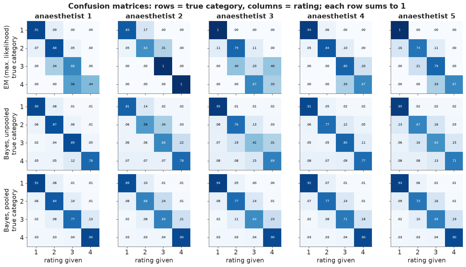
EM fits each confusion row from whatever patients happen to be in that category. For the rare true categories rows are 0s and 1s (anaesthetist 2 "always" rates a category-3 patient 3, anaesthetist 3 "always" rates a category-1 patient 1), and 38 of the 80 entries are exactly zero - "never" from a handful of patients. The unpooled Bayesian fit keeps every entry away from 0 and 1; its row 4, estimated from about two patients, says little beyond the prior. The pooled fit borrows across anaesthetists: the between-rater sd $\tau$ is modest (posterior median 0.38 on the logit scale, 90% interval 0.08-0.71), so the five matrices are pulled toward one shared pattern. Row 4 is then essentially the same for everyone (0.90 on the diagonal) - an honest reading is that the data say almost nothing about how each anaesthetist rates the sickest patients; the pooled model reports the shared matrix, which itself leans on the diagonal-favouring prior. The common structure is sensible for an ordinal scale: errors are mostly to an adjacent category.
7.3 · Checks
Two predictive checks aimed at the model's assumptions: the agreement of each pair of raters, and anaesthetist 1's self-agreement across his three readings (conditional independence says repeated readings of the same form are independent given the truth, which a rater who remembers the form would violate).
def replicate_ds(idata, M_items, rater_, n_items, n_rep=1000, seed=3):
    g = np.random.default_rng(seed)
    pi_d_, th_d = draws(idata, "pi"), draws(idata, "theta")
    idx_ = g.choice(len(pi_d_), n_rep, replace=False)
    true = (g.random((n_rep, n_items, 1)) > np.cumsum(pi_d_[idx_], axis=1)[:, None, :]).sum(axis=2)
    true_r = true[:, M_items]                                 # (rep, ratings)
    probs = th_d[idx_][np.arange(n_rep)[:, None], rater_[None, :], true_r]   # (rep, ratings, K)
    return (g.random(probs.shape[:2] + (1,)) > np.cumsum(probs, axis=2)).sum(axis=2), true


item_of = item
lab_rep, _ = replicate_ds(ds_fits["pooled"], item_of, rater, I_A)


def ds_stats(labs):
    """(..., ratings) -> anaesthetist 1 self-agreement and mean pairwise agreement of raters 2-5."""
    labs = np.atleast_2d(labs)
    r1_ = np.stack([labs[:, (item == i) & (rater == 0)] for i in range(I_A)], axis=1)
    self_agree = (r1_.min(axis=2) == r1_.max(axis=2)).mean(axis=1)
    single = np.stack([np.stack([labs[:, (item == i) & (rater == j)][:, 0] for i in range(I_A)], 1)
                       for j in range(1, J_A)], axis=2)       # (rep, item, rater 2-5)
    pa = np.stack([(single[..., a] == single[..., b]).mean(axis=1)
                   for a, b in combinations(range(J_A - 1), 2)], axis=1)
    return self_agree, pa


sa_obs, pa_obs = ds_stats(lab)
sa_rep, pa_rep = ds_stats(lab_rep)
print(f"anaesthetist 1 self-agreement: observed {sa_obs[0]:.2f}, replicated 90% "
      f"{q(sa_rep)[[0, 2]]}, P(rep >= obs) = {np.mean(sa_rep >= sa_obs[0]):.2f}")
zp = (pa_obs[0] - pa_rep.mean(axis=0)) / pa_rep.std(axis=0)
print("pairwise agreement of anaesthetists 2-5, z-scores (obs - rep):", zp.round(2))
anaesthetist 1 self-agreement: observed 0.71, replicated 90% [0.511 0.8  ], P(rep >= obs) = 0.31
pairwise agreement of anaesthetists 2-5, z-scores (obs - rep): [-0.36  0.44 -0.3  -0.3   0.37  0.07]
Anaesthetist 1 agrees with himself about as often as the model predicts for three independent readings, so there is no sign that he remembered the forms, and the pairwise agreements among the other four fall within the replicated range. With 45 patients these checks can only catch large violations.
7.4 · The patients: majority vote vs the model
p_true = ds_fits["pooled"].posterior["p_true"].mean(("chain", "draw")).to_numpy()
p_unp = ds_fits["unpooled"].posterior["p_true"].mean(("chain", "draw")).to_numpy()
model_lab = p_true.argmax(axis=1)
disagree = np.where((model_lab != mv_a) | ties)[0]
unsure = np.where(p_true.max(axis=1) < 0.9)[0]
print(f"patients where the pooled model's most probable category differs from majority vote or MV "
      f"ties: {(disagree + 1).tolist()}")
print(f"patients with max posterior probability < 0.9: {(unsure + 1).tolist()}")
print(f"pooled vs unpooled most-probable category differ for {int((p_unp.argmax(1) != model_lab).sum())} patients")
show = np.union1d(disagree, unsure)
print(pd.DataFrame(np.column_stack([counts[show].astype(int), p_true[show].round(2)]),
                   index=[f"patient {i + 1}" for i in show],
                   columns=[f"votes {k}" for k in range(1, 5)] + [f"P(true={k})" for k in range(1, 5)]))
for i in disagree:
    print(f"patient {i + 1}: ratings by anaesthetist", {j + 1: (lab[(item == i) & (rater == j)] + 1).tolist()
                                                        for j in range(J_A)})
patients where the pooled model's most probable category differs from majority vote or MV ties: [12, 38]
patients with max posterior probability < 0.9: [3, 12, 38]
pooled vs unpooled most-probable category differ for 0 patients
            votes 1  votes 2  votes 3  votes 4  P(true=1)  P(true=2)  \
patient 3       3.0      4.0      0.0      0.0       0.29       0.71
patient 12      0.0      3.0      3.0      1.0       0.00       0.68
patient 38      0.0      3.0      4.0      0.0       0.00       0.75

            P(true=3)  P(true=4)
patient 3        0.00        0.0
patient 12       0.32        0.0
patient 38       0.25        0.0
patient 12: ratings by anaesthetist {1: [2, 2, 2], 2: [3], 3: [3], 4: [4], 5: [3]}
patient 38: ratings by anaesthetist {1: [2, 3, 2], 2: [3], 3: [2], 4: [3], 5: [3]}fig, ax = plt.subplots(figsize=(14, 3.6))
ordr = np.lexsort((-p_true.max(axis=1), model_lab))
cols4 = [AQUA, BLUE, ORANGE, RED]
bottom = np.zeros(I_A)
for k in range(K_A):
ax.bar(np.arange(I_A), p_true[ordr, k], bottom=bottom, color=cols4[k], width=0.85,
label=f"true category {k + 1}")
bottom += p_true[ordr, k]
for x, i in enumerate(ordr):
ax.text(x, 1.02, str(mv_a[i] + 1) + ("*" if ties[i] else ""), ha="center", fontsize=7)
ax.set_xticks(np.arange(I_A), ordr + 1, fontsize=6)
ax.set(xlabel="patient", ylabel="posterior probability", ylim=(0, 1.1), xlim=(-0.6, I_A + 5.5),
title="Each patient's true category (pooled Dawid-Skene); numbers above = majority vote (* tie)")
ax.legend(fontsize=7, loc="center right");
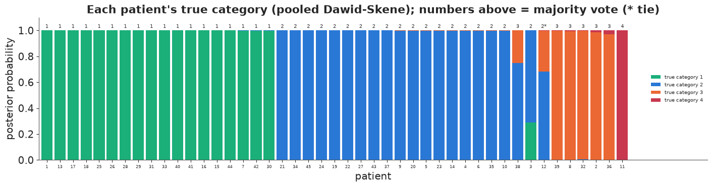
For 42 of the 45 patients the model and the majority agree and the model is at least 90% sure. Three patients are genuinely split between adjacent categories. Patient 12 is a majority-vote tie (anaesthetist 1 said 2 three times; three others said 3 and one said 4); patient 38 has four votes for 3 and three for 2, yet the model prefers 2 (0.75). Both times it leans on anaesthetist 1, the most reliable rater for true category 2 (he rates such a patient 3 about 10% of the time; anaesthetists 2, 4 and 5 do so 14-24% of the time). Majority vote counts his three readings as three votes; the model counts them as three noisy readings by one rater. Pooled and unpooled fits pick the same most probable category for every patient.
8 · A known-truth check (simulated)
Everything so far is inference about a truth we never see. To check that the machinery is calibrated, simulate a dataset from the fitted pooled model with a known true category for each of 600 patients, refit, and compare with the truth. With all seven ratings per patient almost every patient is easy, so we simulate the cheaper design typical of crowdsourcing: each patient is rated once by three of the five anaesthetists, chosen at random. We also score majority vote.
N_SIM, PER = 600, 3
g = np.random.default_rng(8)
pi_true = draws(ds_fits["pooled"], "pi").mean(axis=0)
th_true = th_pool
true_sim = g.choice(K_A, N_SIM, p=pi_true)
item_s = np.repeat(np.arange(N_SIM), PER)
rater_s = np.concatenate([g.choice(J_A, PER, replace=False) for _ in range(N_SIM)])
lab_s = np.array([g.choice(K_A, p=th_true[r_, true_sim[i_]]) for i_, r_ in zip(item_s, rater_s)])
M_S = np.zeros((N_SIM, len(item_s)))
M_S[item_s, np.arange(len(item_s))] = 1.0
t0 = time.time()
with dawid_skene(M_S, rater_s, lab_s, N_SIM, pooled=True):
    idata_sim = pm.sample(random_seed=RANDOM_SEED, progressbar=False, target_accept=0.9)
print(f"{time.time() - t0:.0f} s; {diag(idata_sim, ['pi', 'theta'])}")

p_sim = idata_sim.posterior["p_true"].mean(("chain", "draw")).to_numpy()
cnt_s = np.zeros((N_SIM, K_A))
np.add.at(cnt_s, (item_s, lab_s), 1)
tie_s = (cnt_s == cnt_s.max(axis=1, keepdims=True)).sum(axis=1) > 1
mv_s = np.array([g.choice(np.flatnonzero(c == c.max())) for c in cnt_s])   # random tie-break
print(f"accuracy vs truth: model {np.mean(p_sim.argmax(1) == true_sim):.3f}, "
      f"majority vote {np.mean(mv_s == true_sim):.3f} (ties broken at random: {tie_s.sum()} patients)")
print(f"log score (mean log P(true label)): model {np.mean(np.log(p_sim[np.arange(N_SIM), true_sim])):.3f}")
th_sim = draws(idata_sim, "theta")
lo, hi = np.quantile(th_sim, [0.05, 0.95], axis=0)
print(f"confusion entries inside their 90% interval: {np.mean((th_true >= lo) & (th_true <= hi)):.0%} "
      f"of {th_true.size}")
4 s; divergences 0, max r_hat 1.002, min bulk ESS 1291
accuracy vs truth: model 0.948, majority vote 0.900 (ties broken at random: 23 patients)
log score (mean log P(true label)): model -0.158
confusion entries inside their 90% interval: 100% of 80
pmax = p_sim.max(axis=1)
correct = p_sim.argmax(axis=1) == true_sim
bins_c = np.array([0.3, 0.5, 0.6, 0.7, 0.8, 0.9, 0.97, 0.995, 1.0001])
which = np.digitize(pmax, bins_c) - 1
fig, axes = plt.subplots(1, 2, figsize=(11, 4))
for b_ in range(len(bins_c) - 1):
    sel = which == b_
    if sel.sum() > 0:
        m_, n_ = correct[sel].mean(), sel.sum()
        se_ = np.sqrt(max(m_ * (1 - m_), 0.01) / n_)
        axes[0].errorbar(pmax[sel].mean(), m_, yerr=1.64 * se_, fmt="o", color=BLUE, capsize=3)
        axes[0].annotate(f"n={n_}", (pmax[sel].mean(), m_), fontsize=7, xytext=(4, -10),
                         textcoords="offset points")
axes[0].plot([0.3, 1], [0.3, 1], color="k", lw=1, ls="--")
axes[0].set(xlabel="model's probability for its most likely category",
            ylabel="share actually correct", title="Calibration against the known truth (simulated)")
axes[1].scatter(th_true.ravel(), th_sim.mean(axis=0).ravel(), s=12, color=PURPLE)
axes[1].vlines(th_true.ravel(), lo.ravel(), hi.ravel(), color=PURPLE, alpha=0.3)
axes[1].plot([0, 1], [0, 1], color="k", lw=1, ls="--")
axes[1].set(xlabel="true confusion probability", ylabel="posterior mean (90% interval)",
            title="Recovering 80 confusion probabilities");
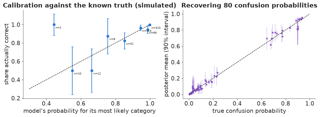
Three findings. First, the label probabilities are calibrated within binomial error: in every bin the share correct is consistent with the stated probability (the bins below 0.8 hold only 2-12 patients each, so this is a coarse check). Second, the model beats majority vote: 94.8% vs 90.0% correct, with 23 majority-vote ties broken at random; reliability weighting matters most exactly where the raters split. Third, all 80 true confusion probabilities lie inside their 90% intervals - more than 90%, because pooling and the prior widen the intervals of rare rows. This is the check to repeat before trusting a latent class model on a new problem: simulate from the fitted model with the real design and see what it recovers. It checks the computation and the design, not the modelling assumptions - data simulated from the model satisfy conditional independence by construction.
9 · Decisions for the carcinoma slides
9.1 · Which slides should an expert panel adjudicate?
Suppose each slide leads to one of two actions: refer (colposcopy and follow-up) or routine screening. Illustrative losses (in units of one unnecessary referral):
| truth \ action | refer | routine |
|---|---|---|
| negative | 1 | 0 |
| ambiguous | 0 | 5 |
| positive | 0 | 20 |
An expert panel can review a slide and (we assume) determine its class, at a cost of 0.5 units. With posterior class probabilities $p_i$ the best action without review has expected loss $\min(p_{i,\text{neg}},\; 5 p_{i,\text{amb}} + 20 p_{i,\text{pos}})$; after a perfect review it is 0. So that minimum is the expected value of perfect information for slide $i$: review it when it exceeds the cost. We use the three-class model, and average the loss over its posterior.
LOSS = np.array([[1.0, 0.0], [0.0, 5.0], [0.0, 20.0]])    # rows: class; cols: refer, routine
COST_REVIEW = 0.5
pcls_d = draws(idata_lc3, "p_cls")                         # (S, item, cls)
pcls = pcls_d.mean(axis=0)
exp_loss = pcls @ LOSS                                      # (item, action)
action = exp_loss.argmin(axis=1)
evpi = exp_loss.min(axis=1)
review = evpi > COST_REVIEW
mv_action = np.where(mv == 1, 0, 1)
print(f"refer {int((action == 0).sum())} slides, routine {int((action == 1).sum())}; majority vote "
      f"would refer {int((mv_action == 0).sum())}")
print(f"slides worth an expert review (EVPI > {COST_REVIEW}): {int(review.sum())}; expected loss "
      f"without reviews {evpi.sum():.1f}, with them {evpi[~review].sum() + COST_REVIEW * review.sum():.1f}")
tab = pd.DataFrame({"pattern": ["".join(map(str, r)) for r in Y], "calls": k_pos,
                    "P(neg)": pcls[:, 0], "P(amb)": pcls[:, 1], "P(pos)": pcls[:, 2],
                    "action": np.where(action == 0, "refer", "routine"), "EVPI": evpi, "review": review})
patt_tab = (tab.groupby("pattern").agg(slides=("calls", "size"), calls=("calls", "first"),
                                       **{c: (c, "first") for c in ["P(neg)", "P(amb)", "P(pos)",
                                                                    "action", "EVPI", "review"]})
            .sort_values("EVPI", ascending=False))
print(patt_tab.round(3).head(10).to_string())
refer 80 slides, routine 38; majority vote would refer 59
slides worth an expert review (EVPI > 0.5): 8; expected loss without reviews 9.0, with them 6.6
         slides  calls  P(neg)  P(amb)  P(pos)   action   EVPI  review
pattern
0100000       6      1   0.828   0.172   0.000    refer  0.828    True
0000100       2      1   0.856   0.144   0.000  routine  0.719    True
1100000       2      2   0.362   0.637   0.000    refer  0.362   False
1000000       2      1   0.944   0.056   0.000  routine  0.278   False
0100100       4      2   0.187   0.813   0.000    refer  0.187   False
0100001       1      2   0.094   0.906   0.000    refer  0.094   False
1100100       2      3   0.019   0.970   0.011    refer  0.019   False
0000000      34      0   0.997   0.003   0.000  routine  0.013   False
1100001       1      3   0.007   0.960   0.032    refer  0.007   False
0100101       5      3   0.002   0.992   0.006    refer  0.002   False
Majority vote refers the 59 slides with 4+ positive calls. The model refers 80: anything with a real chance of being ambiguous or positive, because missing those is expensive. The slides worth a review are not the 3-4 splits - the model is confident those are ambiguous and refers them anyway - but the 8 slides on which a single liberal reader (B or E) called carcinoma: probably negative (P about 0.83-0.86), with a 14-17% chance of an ambiguous lesion. Reviewing them cuts the expected loss over all 118 slides from 9.0 to 6.6 units. Unanimous slides are never worth a review.
The list is only as good as the model. The random-effects model of section 5.1, which gives a unanimously negative slide a 27% chance of carcinoma, would make every one of the 34 unanimous negatives worth a review (routine would cost $20 \times 0.27$ in expectation, referral 0.73, so a perfect review is worth 0.73 > 0.5). Choosing the latent class model is a clinical statement about what "carcinoma" means, not only a statistical one.
9.2 · Which three pathologists to keep?
A lab can afford three readers per slide in future. Which three? For every one of the 35 panels, compute from the three-class model the expected loss per slide of the best refer/routine rule based on that panel's calls alone: enumerate the 8 call patterns, their probabilities under each class, choose the Bayes action per pattern, and average over classes and posterior draws. The answer depends on the loss table, so we compute it for two: the one above (missing an ambiguous slide costs 5) and a "carcinoma only" table in which missing an ambiguous slide costs no more than an unnecessary referral (1).
LOSSES = {"missed ambiguous = 5": LOSS,
          "missed ambiguous = 1": np.array([[1.0, 0.0], [0.0, 1.0], [0.0, 20.0]])}
w_d = draws(idata_lc3, "w")[::4]                            # thin draws: (S', cls)
r_d = rate_d[::4]                                          # (S', rater, cls)


def panel_loss(panel, loss):
    pats = np.array(np.meshgrid(*[[0, 1]] * len(panel), indexing="ij")).reshape(len(panel), -1).T
    rr = r_d[:, panel, :]                                  # (S', p, cls)
    lik = np.prod(np.where(pats[None, :, :, None] == 1, rr[:, None], 1 - rr[:, None]), axis=2)
    joint = lik * w_d[:, None, :]                          # (S', pattern, cls)
    rule = (joint.mean(axis=0) @ loss).argmin(axis=1)      # Bayes action per pattern
    return np.einsum("spc,pc->s", joint, loss[:, rule].T)  # expected loss per draw


panels = {}
for lname, loss in LOSSES.items():
    rows_ = []
    for panel in combinations(range(J), 3):
        ld = panel_loss(list(panel), loss)
        rows_.append(("".join(RATERS[j] for j in panel), ld.mean(), *np.quantile(ld, [0.05, 0.95])))
    res = pd.DataFrame(rows_, columns=["panel", "loss", "lo", "hi"]).sort_values("loss")
    single = pd.Series({RATERS[j]: panel_loss([j], loss).mean() for j in range(J)})
    no_info = (w_d.mean(axis=0) @ loss).min()              # best action with no reader at all
    full = panel_loss(list(range(J)), loss).mean()
    best = res.panel.iloc[0]
    ld_best = panel_loss([RATERS.index(c) for c in best], loss)
    p_beat = {p_: round(float(np.mean(ld_best < panel_loss([RATERS.index(c) for c in p_], loss))), 2)
              for p_ in res.panel.iloc[1:4]}
    panels[lname] = dict(res=res.reset_index(drop=True), single=single, no_info=no_info, full=full)
    print(f"[{lname}] no reader {no_info:.3f}, best single {single.idxmin()} {single.min():.3f}, "
          f"all seven {full:.3f} per slide")
    print("   best panels:", ", ".join(f"{r.panel} {r.loss:.3f}" for r in res.head(5).itertuples()),
          "| worst:", ", ".join(f"{r.panel} {r.loss:.3f}" for r in res.tail(3).itertuples()))
    print(f"   P(best panel {best} beats the next three):", p_beat)
[missed ambiguous = 5] no reader 0.373, best single B 0.290, all seven 0.066 per slide
   best panels: BEG 0.085, BCG 0.088, BFG 0.088, BDG 0.088, ABG 0.088 | worst: ADF 0.373, CDF 0.373, ACD 0.373
   P(best panel BEG beats the next three): {'BCG': 0.53, 'BFG': 0.51, 'BDG': 0.51}
[missed ambiguous = 1] no reader 0.373, best single G 0.182, all seven 0.022 per slide
   best panels: BEG 0.035, ABE 0.044, EFG 0.048, DEG 0.048, CEG 0.048 | worst: ACF 0.117, ADF 0.130, CDF 0.373
P(best panel BEG beats the next three): {'ABE': 0.76, 'EFG': 0.82, 'DEG': 0.82}fig, axes = plt.subplots(2, 1, figsize=(13, 7.5))
for ax, (lname, d_) in zip(axes, panels.items()):
res = d_["res"]
ax.vlines(np.arange(len(res)), res.lo, res.hi, color=BLUE, alpha=0.5, lw=3)
ax.scatter(np.arange(len(res)), res.loss, color=BLUE, s=18, zorder=3, label="3-reader panel")
ax.axhline(d_["full"], color=AQUA, ls="--", label="all seven pathologists")
ax.axhline(d_["single"].min(), color=GREY, ls=":", label=f"best single reader ({d_['single'].idxmin()})")
ax.axhline(d_["no_info"], color=RED, lw=1, label="no reader (best blanket action)")
ax.set_xticks(np.arange(len(res)), res.panel, rotation=90, fontsize=7)
ax.set(ylabel="expected loss per slide", title=f"Which three pathologists to keep? Loss table: {lname}")
ax.legend(fontsize=7, loc="upper left");
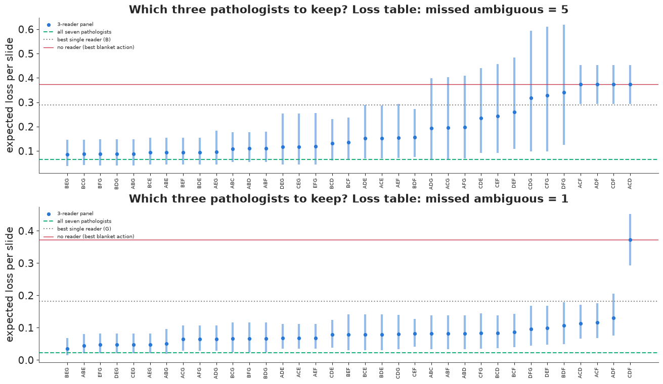
The same three pathologists come out on top under both loss tables: B, E and G. They are the readers who flag the ambiguous slides (they call them positive 92%, 76% and 64% of the time) while rarely calling a clearly negative slide positive. With "missed ambiguous = 5" their panel costs 0.085 per slide against 0.066 for all seven, but four other panels containing B and G are within 0.003 and beat BEG in about half of the posterior draws: choose among them on cost or availability. With "missed ambiguous = 1" the ranking is sharper (BEG beats the next panels in 76-82% of draws).
The conservative readers C, D and F are of little use for this decision: under the first loss table the panels ACD, ACF, ADF and CDF are no better than referring every slide without looking, because their "negative" calls cannot rule out an ambiguous lesion. What a rater is worth depends on the decision, not only on an accuracy score.
Summary
- Majority vote assumes equal, symmetric, certain raters. The latent class model replaces
those assumptions with parameters: prevalence and per-rater sensitivity/specificity (or a full
confusion matrix), with the true class summed out with
logsumexp. - Identifiability first: count degrees of freedom ($2^J - 1$) against parameters. Two
binary raters identify only bounds, unless a second population has a different prevalence
(Hui-Walter; shown on simulated data) or informative priors bear on the unidentified direction
- in which case the conclusion belongs to the priors.
- Label switching is an exact symmetry. Mirrored chains gave a huge r_hat with zero divergences; a "better than chance" parameterisation ($\mathrm{Se} = \mathrm{fpr} + (1 - \mathrm{fpr})u$; ordered class logits; a diagonal-favouring confusion prior) removes it.
- Conditional independence failed a score / pairwise-agreement check on the carcinoma slides. A random-effects model fixed the fit (+20 nats LOO) but turned the class into something other than carcinoma (P = 0.27 for a slide nobody called positive); a three-class model with an "ambiguous" class fitted as well and kept its meaning. With no gold standard, fit is necessary but not sufficient: check what the latent class means.
- Dawid-Skene with pooled confusion matrices avoids EM's zeros and ones for rare categories, although for the rarest category the pooled matrix is mostly prior; checks on self-agreement and pairwise agreement passed; a simulation from the fitted model (three ratings per patient) showed calibrated label probabilities and 95% vs 90% accuracy over majority vote.
- Decisions use the posterior directly: the value of information ranks slides for expert review (lone positive calls, not the 3-4 splits), and the expected loss of every three-reader panel picks the readers to keep (B, E, G: the ones who flag ambiguous slides).
Try it yourself
- Class-specific random effects. Give the random-effects model of section 5.1 a separate scale for each class (as Qu, Tan & Kutner did), or restrict the random effect to the positive class only. Does the latent class keep its meaning, and how do the sensitivities compare with the three-class model?
- Four classes and LOO. Fit a four-class version of section 5.2 (four raters are needed per the table in 6.1; there are seven). Does LOO prefer it, and do the adjudication decisions of section 9.1 change?
- Adaptive rating with Dawid-Skene. In the simulated design of section 8, start with ONE rating per patient and add ratings one at a time, always asking a new anaesthetist about the patient whose posterior class probabilities have the highest entropy (refit every 100 ratings). How many ratings does it take to match the accuracy of three ratings for everyone?