The setting
A topic model describes a collection of documents as mixtures of a few recurring themes. Latent Dirichlet allocation (Blei, Ng & Jordan 2003) says:
- there are $K$ topics; topic $k$ is a probability distribution $\phi_k$ over a vocabulary of $V$ words;
- each document $d$ has its own mixture $\theta_d$ over the topics;
- each token in document $d$ is made by first drawing a topic $z \sim \theta_d$ and then a word $w \sim \phi_z$.
Nothing in this story needs the "words" to be words. All LDA sees is a table of counts: how often did feature $w$ occur in unit $d$. Any data of that shape can be read as documents made of a few mixed "themes":
| domain | document | "word" | a topic is... |
|---|---|---|---|
| text | article, headline set | word | a theme |
| images, creatives, magazine covers | an image | a quantised colour (or visual word) | a palette |
| retail | a shopping basket or customer | product | a shopping mission |
| population genetics | a person's genome | allele at a locus | an ancestral population (the STRUCTURE model of Pritchard, Stephens & Donnelly 2000 is LDA) |
| microbiome | a sample | bacterial taxon | a community type |
| web analytics | a user session | page or event | a browsing intent |
| music | a playlist | track or chord | a style |
This notebook fits LDA to two such collections and, in each case, uses the topics for something:
| part | question | tool |
|---|---|---|
| A | What is LDA, and can PyMC fit it? | marginalised likelihood, simulated check, label switching |
| B | What are Upworthy's stories about? | collapsed Gibbs sampler, stability across restarts; four displays of word topics |
| C | How many topics, and do topics predict clicks? | held-out likelihood vs downstream prediction, regression with uncertain regressors |
| D | How do you turn a poster into a document? | CIELab colour vocabulary, pixels as tokens |
| E | Which palettes recur across 750 posters? | Gibbs restarts, palette stability; four displays of palettes |
| F | How did palettes change from the 1890s to the WPA, and when was this poster made? | logistic-normal vs Dirichlet era models, semi-supervised dating, calibration |
| G | How much is a picture worth? | the number of tokens per image and what it does to certainty |
| H | And for web sessions and shopping baskets? | browsing intents on msnbc.com; shopping missions of an online retailer, by market; predicting the rest of a visit and recommending products against baselines |
import logging
import time
import warnings

import arviz as az
import matplotlib.pyplot as plt
import numba
import numpy as np
import pandas as pd
import pymc as pm
import pytensor.tensor as pt
import re
from collections import Counter
from scipy.optimize import linear_sum_assignment

from pymc_challenges import data

RANDOM_SEED = 72
rng = np.random.default_rng(RANDOM_SEED)
az.style.use("arviz-variat")
logging.getLogger("pymc").setLevel(logging.WARNING)
warnings.filterwarnings("ignore", category=RuntimeWarning, module="arviz")
pd.set_option("display.width", 170)
pd.set_option("display.max_columns", 20)
A. The model, and a check on simulated data
Written out for one document with counts $n_{dw}$ (how often word $w$ appears in document $d$), the token-level topic labels $z$ can be summed out: a token is word $w$ with probability
$$p_{dw} = \sum_{k=1}^K \theta_{dk}\,\phi_{kw}, \qquad \text{so} \qquad \mathbf n_d \sim \text{Multinomial}\big(N_d,\; \boldsymbol\theta_d^\top \Phi\big).$$
That is a plain multinomial with a low-rank probability matrix $\Theta\Phi$ ($D \times V$, rank $K$): LDA is a non-negative matrix factorisation of the count table with a multinomial likelihood and Dirichlet priors. With $z$ gone every parameter is continuous, so NUTS can run. The priors are
$$\boldsymbol\theta_d \sim \text{Dirichlet}(\alpha\mathbf 1_K), \qquad \boldsymbol\phi_k \sim \text{Dirichlet}(\beta\mathbf 1_V),$$
with $\alpha < 1$ saying "a document is mostly about a few topics" and $\beta < 1$ saying "a topic uses a small part of the vocabulary".
Before any real data, check the machinery on a corpus where we know the answer: 200 documents of 60 tokens over a 24-word vocabulary, made from 3 topics.
D_sim, V_sim, K_sim, N_sim = 200, 24, 3, 60
phi_true = rng.dirichlet(np.full(V_sim, 0.3), K_sim)
theta_true = rng.dirichlet(np.full(K_sim, 0.5), D_sim)
X_sim = np.array([rng.multinomial(N_sim, theta_true[d] @ phi_true) for d in range(D_sim)])

with pm.Model(coords={"doc": range(D_sim), "topic": range(K_sim), "word": range(V_sim)}) as lda_sim:
    theta = pm.Dirichlet("theta", a=np.full(K_sim, 0.5), dims=("doc", "topic"))
    phi = pm.Dirichlet("phi", a=np.full(V_sim, 0.5), dims=("topic", "word"))
    pm.Multinomial("x", n=N_sim, p=theta @ phi, observed=X_sim, dims=("doc", "word"))
    idata_sim = pm.sample(random_seed=RANDOM_SEED, progressbar=False)

print("divergences:", int(idata_sim.sample_stats["diverging"].sum()))
print("largest r_hat of phi, as sampled:", round(float(az.rhat(idata_sim.posterior["phi"]).max()), 2))
divergences: 0
largest r_hat of phi, as sampled: 1.75
Zero divergences, yet $\hat R$ is far above 1. The reason is not a sampling failure: the
likelihood is unchanged if the topics are relabelled, so "topic 0" in one chain can be "topic 2"
in another. This is label switching, and every mixture and topic model has it. NUTS rarely
switches labels within a chain (the modes are far apart), so the fix is to match topics
across chains: compute a cost for pairing topic $j$ of one chain with topic $k$ of a reference
chain (here the squared distance between their word distributions) and solve the assignment
problem (scipy.optimize.linear_sum_assignment, the Hungarian algorithm).
def align_to(ref, other):
    """Permutation `perm` such that other[perm] best matches ref (rows are topics)."""
    cost = ((ref[:, None, :] - other[None, :, :]) ** 2).sum(-1)
    return linear_sum_assignment(cost)[1]


def align_chains(phi_draws):
    """phi_draws: (chain, draw, topic, word). Returns one permutation per chain (chain 0 = reference)."""
    means = phi_draws.mean(1)
    return np.array([align_to(means[0], means[c]) for c in range(len(means))])


phi_s = idata_sim.posterior["phi"].values
perms_sim = align_chains(phi_s)
print("topic permutation per chain:\n", perms_sim)
phi_aligned = np.stack([phi_s[c][:, perms_sim[c]] for c in range(phi_s.shape[0])])
theta_s = idata_sim.posterior["theta"].values
theta_aligned = np.stack([theta_s[c][:, :, perms_sim[c]] for c in range(theta_s.shape[0])])
rhat_aligned = az.rhat(np.asarray(phi_aligned).reshape(phi_aligned.shape[0], phi_aligned.shape[1], -1))
print("largest r_hat of phi after alignment:", round(float(np.max(rhat_aligned)), 3))

# match the fitted topics to the true ones for the plot
to_true = align_to(phi_true, phi_aligned.mean((0, 1)))
phi_fit = phi_aligned.mean((0, 1))[to_true]
theta_fit = theta_aligned.mean((0, 1))[:, to_true]

fig, axes = plt.subplots(1, 2, figsize=(11, 3.6))
for k in range(K_sim):
    axes[0].plot(phi_true[k], "o-", color=f"C{k}", lw=1, label=f"topic {k}, true")
    axes[0].plot(phi_fit[k], "x", color=f"C{k}", ms=8)
axes[0].set(xlabel="word", ylabel="probability within topic", title="Topics: true (o) and posterior mean (x)")
axes[0].legend(fontsize=8)
axes[1].scatter(theta_true.ravel(), theta_fit.ravel(), s=6, alpha=0.5)
axes[1].plot([0, 1], [0, 1], color="k", lw=0.8)
axes[1].set(xlabel="true topic share", ylabel="posterior mean share", title="Document mixtures (200 docs x 3 topics)");
topic permutation per chain:
 [[0 1 2]
 [0 1 2]
 [1 2 0]
 [1 2 0]]
largest r_hat of phi after alignment: 1.008
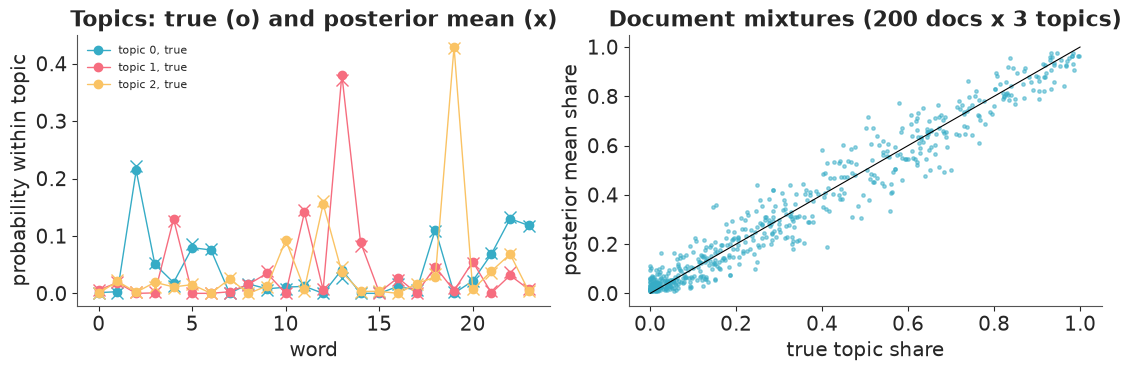
After alignment the chains agree, and both the topics and the per-document mixtures are recovered. Two things to remember for the real data:
- Always align before diagnosing. Raw $\hat R$ on topics measures the arbitrary labelling.
- Alignment only fixes permutations. Real corpora also have genuinely different local solutions - two chains that split the same material into topics differently. No permutation fixes that, and we will meet it in the text.
B. What are Upworthy's stories about?
Upworthy (2013-2015) tested several headlines for every story it published and showed each visitor one of them at random. The archive has 4,873 tests from its exploratory sample (E66 used it for A/B testing). A document here is one test: all the distinct headlines written for one story, pooled. That makes the topics about stories, not about the wording of one headline.
Preparing text for LDA is a bag-of-words recipe: lower-case, split into words, drop "stopwords" (the, you, this, which every topic would otherwise share), fold plurals onto singulars when both are common, and keep words that appear in at least 20 tests but in no more than 10% of them (rare words cannot be learned; ubiquitous ones say nothing).
data.describe("upworthy_exploratory")
uw = data.load("upworthy_exploratory")

STOP = set("""a about above after again against all am an and any are aren't as at be because been before
being below between both but by can can't cannot could couldn't did didn't do does doesn't doing don't down
during each few for from further had hadn't has hasn't have haven't having he he'd he'll he's her here here's
hers herself him himself his how how's i i'd i'll i'm i've if in into is isn't it it's its itself let's me
more most mustn't my myself no nor not of off on once only or other ought our ours ourselves out over own same
shan't she she'd she'll she's should shouldn't so some such than that that's the their theirs them themselves
then there there's these they they'd they'll they're they've this those through to too under until up very
was wasn't we we'd we'll we're we've were weren't what what's when when's where where's which while who who's
whom why why's with won't would wouldn't you you'd you'll you're you've your yours yourself yourselves just
like get gets got one two really thing things way ever even also make makes made know see go going goes say
says said will new something every much many want wants yes""".split())


def tokens(headline):
    words = re.findall(r"[a-z][a-z']+", headline.lower().replace("’", "'"))
    return [w for w in words if w not in STOP and len(w) > 2]


heads = uw.drop_duplicates(["test_id", "headline"])
docs = heads.groupby("test_id")["headline"].apply(lambda h: sum((tokens(x) for x in h), []))
doc_freq = Counter(w for d in docs for w in set(d))
fold = {w: w[:-1] for w in doc_freq if w.endswith("s") and doc_freq.get(w[:-1], 0) >= 20}
docs = docs.map(lambda d: [fold.get(w, w) for w in d])
doc_freq = Counter(w for d in docs for w in set(d))
vocab = np.array(sorted(w for w, c in doc_freq.items() if 20 <= c <= 0.1 * len(docs)))
w_index = {w: i for i, w in enumerate(vocab)}
X_all = np.zeros((len(docs), len(vocab)), dtype=np.int64)
for d, ws in enumerate(docs):
    for w in ws:
        if w in w_index:
            X_all[d, w_index[w]] += 1
keep = X_all.sum(1) >= 3
X_txt, test_ids = X_all[keep], docs.index.to_numpy()[keep]
print(f"{len(docs)} tests, vocabulary of {len(vocab)} words; {keep.sum()} tests keep >= 3 tokens")
print(f"tokens per test: median {np.median(X_txt.sum(1)):.0f}, total {X_txt.sum():,}")
print("most common kept words:", ", ".join(vocab[np.argsort(-X_txt.sum(0))[:25]]))
upworthy_exploratory: Exploratory sample of Upworthy's headline A/B tests, Jan 2013 - Apr 2015: 4,873 tests, 22,666 packages (arms; 2-14 per test, mostly 4-6), one row per package: test_id (clickability_test_id), test_created (date of the test's first package), test_week (YYYYWW), arm (0.. within test, by creation time), content_id (arms of one test with the same id are identical in headline, image, excerpt, lede, share text and square image: natural A/A arms), headline, eyecatcher_id (image), impressions, clicks, significance (Upworthy's dashboard number), first_place, winner (editor's declared winner).
  source: Matias, Munger, Aubin Le Quere & Ebersole (2021), The Upworthy Research Archive, a time series of 32,487 experiments in U.S. media, Scientific Data 8:195 (doi:10.1038/s41597-021-00934-7); OSF project jd64p (CC BY 4.0), file upworthy-archive-exploratory-packages-03.12.2020.csv (the URL). TRIMMED: kept the columns below, dropped excerpt/lede/share text/image URL/slug, added arm and content_id, so keep the cached file in data/.
  url:    https://osf.io/download/3vqmp/
4873 tests, vocabulary of 652 words; 4468 tests keep >= 3 tokens
tokens per test: median 9, total 52,590
most common kept words: kid, women, think, year, guy, time, world, girl, watch, look, video, now, right, reason, take, life, need, woman, never, old, might, gay, good, little, word
Documents are short: a median of about a dozen kept tokens. That is typical of headlines, tweets, search queries, product titles and survey answers, and it matters: each document says little about its own mixture, so topics must be learned from co-occurrence across thousands of documents.
NUTS does not scale here - a collapsed Gibbs sampler does
The PyMC model of part A has $D(K-1) + K(V-1)$ continuous parameters: about 30,000 for this corpus with $K = 6$. While preparing this notebook, we ran it on a random 800 of these tests with $K = 6$, $\alpha = 0.5$, $\beta = 0.1$: it took 6 minutes, gave 517 divergences, hit the maximum tree depth in three quarters of the transitions, and the four chains found four different sets of topics. Sparse Dirichlet priors over hundreds of words put mass in corners that NUTS cannot reach smoothly (AUTHORING notes the same for sparse Dirichlet mixtures).
The standard tool for LDA is the collapsed Gibbs sampler (Griffiths & Steyvers 2004). It does the opposite of part A: it keeps the discrete $z$ and integrates out $\theta$ and $\phi$ (Dirichlet-multinomial conjugacy). Each token's topic is then resampled from
$$P(z_i = k \mid \mathbf z_{-i}) \;\propto\; (n_{dk}^{-i} + \alpha)\, \frac{n_{kw}^{-i} + \beta}{n_k^{-i} + V\beta},$$
where the $n$ are counts of tokens assigned to topic $k$ in document $d$, of word $w$ in topic $k$, and in topic $k$ overall, all excluding token $i$. One sweep over the 50,000 tokens takes milliseconds in Numba. Posterior draws of $\phi$ and $\theta$ come from their Dirichlet full conditionals given the counts at saved sweeps.
@numba.njit
def _gibbs_sweeps(doc, word, z, ndk, nkw, nk, alpha, beta, n_sweeps, seed):
    np.random.seed(seed)
    K, V = nkw.shape
    cum = np.empty(K)
    for _ in range(n_sweeps):
        for i in range(doc.shape[0]):
            d, w, k = doc[i], word[i], z[i]
            ndk[d, k] -= 1
            nkw[k, w] -= 1
            nk[k] -= 1
            total = 0.0
            for j in range(K):
                total += (ndk[d, j] + alpha) * (nkw[j, w] + beta) / (nk[j] + V * beta)
                cum[j] = total
            u = np.random.random() * total
            k = 0
            while cum[k] < u:
                k += 1
            z[i] = k
            ndk[d, k] += 1
            nkw[k, w] += 1
            nk[k] += 1


def lda_gibbs(X, K, alpha=0.1, beta=0.05, burn=2000, draws=40, thin=10, seed=0):
    """Collapsed Gibbs LDA on a document x word count matrix.

    Returns posterior draws of phi (draw, topic, word) and theta (draw, doc, topic), and the
    log-likelihood of the tokens at each saved sweep.
    """
    g = np.random.default_rng(seed)
    d_i, w_i = np.nonzero(X)
    n = X[d_i, w_i]
    doc, word = np.repeat(d_i, n), np.repeat(w_i, n)
    z = g.integers(K, size=doc.size)
    D, V = X.shape
    ndk, nkw = np.zeros((D, K), np.int64), np.zeros((K, V), np.int64)
    np.add.at(ndk, (doc, z), 1)
    np.add.at(nkw, (z, word), 1)
    nk = nkw.sum(1)
    _gibbs_sweeps(doc, word, z, ndk, nkw, nk, alpha, beta, burn, seed)
    phis, thetas, lls = [], [], []
    for s in range(draws):
        _gibbs_sweeps(doc, word, z, ndk, nkw, nk, alpha, beta, thin, seed + 1 + s)
        phi_s = g.gamma(nkw + beta)
        theta_s = g.gamma(ndk + alpha)
        phis.append(phi_s / phi_s.sum(1, keepdims=True))
        thetas.append(theta_s / theta_s.sum(1, keepdims=True))
        lls.append(np.sum(X * np.log(thetas[-1] @ phis[-1])))
    return np.array(phis), np.array(thetas), np.array(lls)


K_TXT = 6
t0 = time.perf_counter()
fits = [lda_gibbs(X_txt, K_TXT, seed=c) for c in range(4)]
print(f"4 chains x 2,400 sweeps: {time.perf_counter() - t0:.1f} s (includes Numba compilation)")
phi_txt = np.stack([f[0] for f in fits])       # chain, draw, topic, word
theta_txt = np.stack([f[1] for f in fits])     # chain, draw, doc, topic
ll_txt = np.stack([f[2] for f in fits])
print("token log-likelihood per chain (mean over saved sweeps):", np.round(ll_txt.mean(1)))
4 chains x 2,400 sweeps: 11.5 s (includes Numba compilation)
token log-likelihood per chain (mean over saved sweeps): [-302356. -301794. -302354. -301947.]
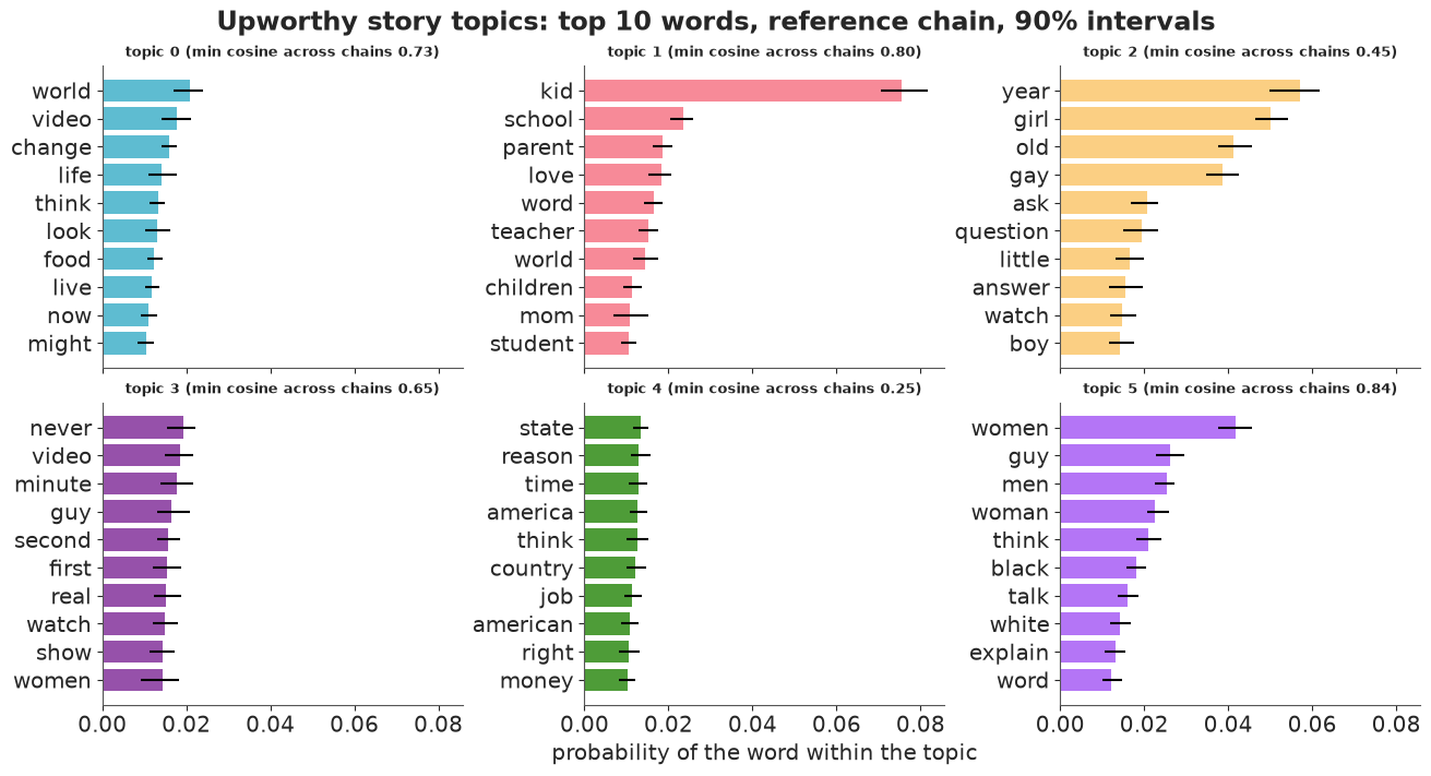
Align the chains as in part A, then ask a question alignment cannot answer by itself: is each topic the same topic in every chain? For each topic of the reference chain we report the cosine similarity of its word distribution to its match in each other chain (1 = identical).
perms_txt = align_chains(phi_txt)
phi_txt = np.stack([phi_txt[c][:, perms_txt[c]] for c in range(4)])
theta_txt = np.stack([theta_txt[c][..., perms_txt[c]] for c in range(4)])
phi_mean_c = phi_txt.mean(1)                    # chain, topic, word


def cosine(a, b):
    return np.sum(a * b, -1) / np.linalg.norm(a, axis=-1) / np.linalg.norm(b, axis=-1)


stability = np.array([cosine(phi_mean_c[0], phi_mean_c[c]) for c in range(1, 4)]).T
labels_txt = [" / ".join(vocab[np.argsort(-phi_mean_c[0, k])[:3]]) for k in range(K_TXT)]
stab = pd.DataFrame(stability.round(2), index=labels_txt, columns=["chain 1", "chain 2", "chain 3"])
stab["min"] = stab.min(axis=1)
print(stab)
                        chain 1  chain 2  chain 3   min
world / video / change     0.73     0.79     0.75  0.73
kid / school / parent      0.80     0.81     0.81  0.80
year / girl / old          0.45     0.81     0.47  0.45
never / video / minute     0.65     0.78     0.66  0.65
state / reason / time      0.84     0.25     0.76  0.25
women / guy / men          0.89     0.88     0.84  0.84
The table is the honest summary of an LDA fit on short texts: some topics come back in every chain and some do not. "women / guy / men" (at least 0.84) and "kid / school / parent" (0.80) are found by every chain; "state / reason / time" has only a loose match (0.25) in one chain and "year / girl / old" (0.45) in two. A stable topic is a real pattern in the co-occurrence of words; an unstable one is one of several equally good ways to cut up the rest. When LDA topics are reported without this check, readers cannot tell which kind they are looking at.
The top words below are from the reference chain, with the posterior uncertainty of each word's probability (a 90% interval over saved sweeps) - the sampling uncertainty is small compared with the chain-to-chain differences above.
fig, axes = plt.subplots(2, 3, figsize=(13, 7), sharex=True)
for k, ax in enumerate(axes.ravel()):
    top = np.argsort(-phi_mean_c[0, k])[:10][::-1]
    lo, hi = np.quantile(phi_txt[0][:, k, top], [0.05, 0.95], axis=0)
    ax.barh(range(10), phi_mean_c[0, k, top], xerr=[phi_mean_c[0, k, top] - lo, hi - phi_mean_c[0, k, top]],
            color=f"C{k}", alpha=0.8)
    ax.set_yticks(range(10), vocab[top])
    ax.set_title(f"topic {k} (min cosine across chains {stab['min'].iloc[k]:.2f})", fontsize=9)
axes[1, 1].set_xlabel("probability of the word within the topic")
fig.suptitle("Upworthy story topics: top 10 words, reference chain, 90% intervals");
A few example stories for each topic: the tests with the largest posterior mean share of it, shown by their first headline.
first_headline = uw.sort_values("arm").groupby("test_id")["headline"].first()
theta_ref = theta_txt[0].mean(0)
for k in range(K_TXT):
    print(f"\ntopic {k}: {labels_txt[k]}")
    for d in np.argsort(-theta_ref[:, k])[:3]:
        print(f"   {theta_ref[d, k]:.2f}  {first_headline[test_ids[d]][:110]}")
topic 0: world / video / change
   0.97  The Cost Of Being A Trendy Eater Hurts A Lot More People Than The Whole Foods Crowd May Realize
   0.97  Watch This Ridiculously Adorable And Uplifting Video Of A Huge Company Actually Doing Good Stuff
   0.97  File This Under Awesome Things About The Universe That I Had No Clue About

topic 1: kid / school / parent
   0.98  Oscar Winner Lupita Nyong’o's Speech On Beauty That Left An Entire Audience Speechless
   0.97  Instead Of Saying She Was 'Born A Boy' Try Saying It Her Way Instead. It Just Rings More True.
   0.97  A Teacher Tells A Story About A Boy In Her Class. It Desperately Needs A Happy Ending.

topic 2: year / girl / old
   0.99  Pink, Ellen, Katy Perry, And A Hockey Player Walk Into A Commercial And Destroy A Silly Argument
   0.98  A 4-Year-Old Girl Asked A Lesbian If She Was A Boy. She Responded The Awesomest Way Possible.
   0.97  A Little Girl Uses A Metaphor To Get You To Think About What Stops Girls From Getting Into Science

topic 3: never / video / minute
   0.98  Something Truly Screwed Up Just Happened In Congress, And You Probably Haven't Heard A Word About It
   0.98  2 Minutes In, Even Demi Lovato Was Overwhelmed. Then 10 Minutes Of Raw Real Truth Came Out.
   0.97  I'm Willing To Wager That You've Never Thought To Fight Homophobia Like This

topic 4: state / reason / time
   0.98  The Gap Raised Their Minimum Wage Even Though The Rest Of The Country Wasn't Really Doing It. Cool.
   0.98  The Most Simple Argument Against Raising The Minimum Wage Might Not Be As Simple As You Think
   0.97  The Most Simple Argument Against Raising The Minimum Wage Might Not Be As Simple As You Think

topic 5: women / guy / men
   0.98  Sexists Think Women Are Bad At Math, But Do They Really Think We Don't Know 77 Is Less Than 100?
   0.98  The Messages These Women Read Would Be Funny If They Were From A Movie. Except They're Not.
   0.98  Is it opposite day? One anchor takes on 'white on white crime' and it's good.
Better ways to look at word topics
A list of top words per topic is the most common display of a topic model, and one of the least informative. It hides four things a reader needs: which words are specific to a topic rather than merely frequent everywhere, how the topics relate to each other (and how stable they are), what a topic looks like inside a real document, and how much of the corpus each topic is, over time. Four displays, one for each. Every figure uses the same colour for the same topic (a categorical palette checked for colour-vision deficiency; every coloured mark also carries a text label).
1. Relevance, not probability (Sievert & Shirley 2014, the "LDAvis" display). Ranking by $\phi_{kw}$ puts corpus-wide words ("video", "think", "time") at the top of several topics. The relevance of word $w$ to topic $k$ blends its probability with its lift, how much more common it is in the topic than in the corpus:
$$r_{kw}(\lambda) = \lambda \log \phi_{kw} + (1 - \lambda) \log \frac{\phi_{kw}}{p_w},$$
with $\lambda = 0.6$, the value their user study found most helpful. Each bar pair then shows the word's estimated count in the topic (coloured) against its count in all tests (grey): a coloured bar that fills its grey bar is a word that belongs to that topic alone.
TOPIC_COLOURS = ["#2a78d6", "#eb6834", "#1baf7a", "#eda100", "#e87ba4", "#008300"]   # fixed order, never cycled
GREY_BAR, INK, MUTED = "#d9d8d3", "#0b0b0b", "#8a8984"

phi_ref = phi_mean_c[0]
word_count = X_txt.sum(0)
p_word = word_count / word_count.sum()
tokens_in_topic = (theta_ref * X_txt.sum(1)[:, None]).sum(0)        # expected tokens per topic
LAMBDA = 0.6
relevance = LAMBDA * np.log(phi_ref) + (1 - LAMBDA) * np.log(phi_ref / p_word)
labels_rel = [" / ".join(vocab[np.argsort(-relevance[k])[:3]]) for k in range(K_TXT)]

fig, axes = plt.subplots(2, 3, figsize=(13, 8))
for k, ax in enumerate(axes.ravel()):
    top = np.argsort(-relevance[k])[:12][::-1]
    ax.barh(range(12), word_count[top], color=GREY_BAR, height=0.72, label="count in all tests")
    ax.barh(range(12), phi_ref[k, top] * tokens_in_topic[k], color=TOPIC_COLOURS[k], height=0.72,
            label="estimated count in this topic")
    ax.set_yticks(range(12), vocab[top])
    ax.set_title(f"topic {k}  ({tokens_in_topic[k] / tokens_in_topic.sum():.0%} of tokens)",
                 fontsize=9, loc="left")
    ax.grid(axis="y", visible=False)
handles, names = axes[0, 0].get_legend_handles_labels()
fig.legend(handles, ["count in all tests", "estimated count in the topic (colour = topic)"], loc="lower center",
           ncol=2, fontsize=9, frameon=False, bbox_to_anchor=(0.5, -0.03))
axes[1, 1].set_xlabel("tokens")
fig.suptitle(f"The 12 most relevant words of each topic (relevance, lambda = {LAMBDA})");
print("top-3 words by probability vs by relevance:")
print(pd.DataFrame({"probability": labels_txt, "relevance": labels_rel}, index=[f"topic {k}" for k in range(K_TXT)]))
top-3 words by probability vs by relevance:
                    probability                relevance
topic 0  world / video / change    change / world / food
topic 1   kid / school / parent    kid / school / parent
topic 2       year / girl / old        year / girl / old
topic 3  never / video / minute  second / never / minute
topic 4   state / reason / time   state / country / wage
topic 5       women / guy / men      women / men / black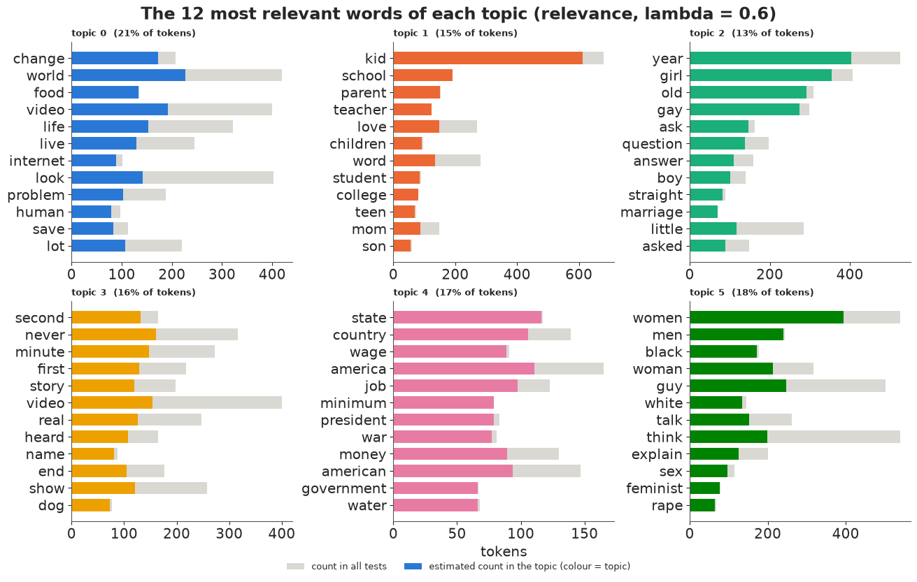
The grey bars expose the generic words: "video", "look", "world", "think", "guy" are frequent in every topic, and a probability ranking lists them first. Relevance brings forward the words that say what a topic is about. Topic 4 is policy ("wage", "minimum", "government", "president", "war", "water"). Topic 2 is not only "year / girl / old" but also "gay", "straight", "marriage": LGBT stories and stories that introduce a person by age share their "ask / question / answer" framing. Topic 5 is gender and race ("black", "white", "feminist", "rape"), and topic 3 is the viral-video topic ("second", "minute", "name", "dog").
2. A map of the topics, with its uncertainty. Topics are distributions over words, so they have distances: the Jensen-Shannon distance between two topics' word distributions (0 = the same words in the same proportions, 1 = no words in common). Classical multidimensional scaling places the topics in a plane so that these distances are kept as well as possible. LDAvis shows only the fitted topics; here the matched topics of all four chains are placed in the same map. A topic whose four versions sit on top of each other is stable, and one whose versions spread out is the fuzzy kind that part B's table warned about. Circle area is the topic's share of the corpus.
def js_distance(P, Q):
    M = 0.5 * (P + Q)
    return np.sqrt(0.5 * np.sum(P * np.log(P / M), -1) + 0.5 * np.sum(Q * np.log(Q / M), -1))


all_topics = phi_mean_c.reshape(-1, len(vocab))                      # (chain x topic) x word
D_js = js_distance(all_topics[:, None], all_topics[None])
n_all = len(D_js)
J = np.eye(n_all) - 1 / n_all
eigval, eigvec = np.linalg.eigh(-0.5 * J @ D_js**2 @ J)
xy = (eigvec[:, -2:] * np.sqrt(eigval[-2:]))[:, ::-1].reshape(4, K_TXT, 2)
share_topic = theta_txt.mean((1, 2))                                    # chain x topic
print(f"MDS keeps {eigval[-2:].sum() / eigval[eigval > 0].sum():.0%} of the squared-distance variation")

fig, ax = plt.subplots(figsize=(8.5, 7))
for k in range(K_TXT):
    for c in range(1, 4):
        ax.plot(*np.c_[xy[0, k], xy[c, k]], color=TOPIC_COLOURS[k], lw=1.2, alpha=0.7, zorder=1)
        ax.scatter(*xy[c, k], s=40, color=TOPIC_COLOURS[k], edgecolor="white", lw=1.5, zorder=3)
    ax.scatter(*xy[0, k], s=share_topic[0, k] * 9000, color=TOPIC_COLOURS[k], alpha=0.25,
               edgecolor=TOPIC_COLOURS[k], lw=2, zorder=2)
    out = xy[0, k] - xy[0].mean(0)                                     # push labels away from the centre
    out = out / np.linalg.norm(out)
    ax.annotate(f"topic {k}\n{labels_rel[k]}", xy[0, k], xytext=out * 62, textcoords="offset points",
                ha="center", va="center", fontsize=8, color=INK,
                bbox=dict(facecolor="white", alpha=0.8, edgecolor="none", pad=1),
                arrowprops=dict(arrowstyle="-", color=MUTED, lw=0.6))
ax.set(xlabel="MDS dimension 1", ylabel="MDS dimension 2", aspect="equal",
       title="Intertopic distance map: big circle = reference chain,\nsmall dots = the same topic in chains 1-3")
ax.margins(0.25);
MDS keeps 37% of the squared-distance variation
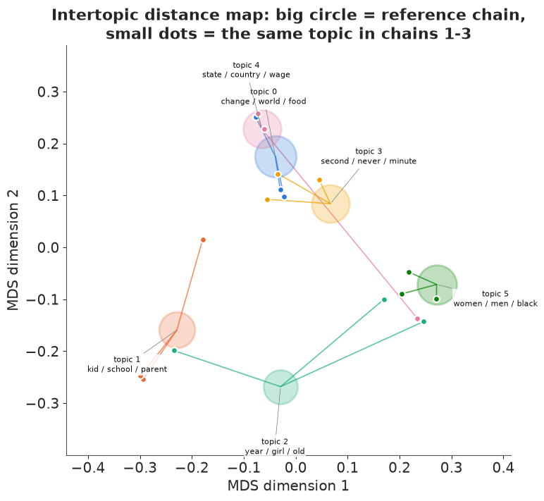
Read the map for neighbourhoods, not exact distances: two dimensions keep only 37% of the distance variation. Topics 1 (kid / school) and 5 (women / men) are tight clusters - all four chains found them. Topics 2 and 4 are not: one chain's version of topic 4 sits next to topic 5, and topic 2's versions are pulled towards topic 5 and topic 1. This is part B's stability table drawn as a picture, and it shows where the unstable topics go: the chains share out the same gender, LGBT and family words in different ways. Topics 0, 3 and 4 crowd the centre because they share the generic "video / world" vocabulary.
3. Topics inside a document. A topic is easiest to understand where it lives. Each headline below has its words highlighted by their most probable topic in that story, which is proportional to $\theta_{dk}\,\phi_{kw}$: the same word can take different topics in different stories. The small bar on the left is the story's topic mix $\theta_d$. Unhighlighted words are stopwords or too rare to be in the vocabulary. We show stories that mix at least two topics.
def headline_tokens(word):
    toks = tokens(word)
    return fold.get(toks[0], toks[0]) if toks else None


two_topic = np.flatnonzero(np.sort(theta_ref, 1)[:, -2] > 0.3)
rows = np.random.default_rng(8).choice(two_topic, 9, replace=False)
fig, ax = plt.subplots(figsize=(13, 0.55 * len(rows) + 1.2))
ax.set(xlim=(0, 1), ylim=(len(rows) - 0.4, -1.2))
ax.axis("off")
renderer = fig.canvas.get_renderer()
to_data = ax.transData.inverted()
for r, d in enumerate(rows):
    left = 0.0
    for k in range(K_TXT):                                        # the story's mixture
        ax.barh(r, theta_ref[d, k] * 0.12, left=left, height=0.5, color=TOPIC_COLOURS[k],
                edgecolor="white", lw=1)
        left += theta_ref[d, k] * 0.12
    x = 0.14
    for word in first_headline[test_ids[d]].split():
        t = ax.text(x, r, word, va="center", fontsize=10, color=INK)
        w = headline_tokens(word)
        if w in w_index:
            k_w = int(np.argmax(theta_ref[d] * phi_ref[:, w_index[w]]))
            t.set_bbox(dict(facecolor=TOPIC_COLOURS[k_w], alpha=0.35, edgecolor="none", pad=1.5))
        else:
            t.set_color(MUTED)
        x = to_data.transform((t.get_window_extent(renderer).x1, 0))[0] + 0.005
x = 0.14
for k in range(K_TXT):                                            # legend row, laid out by measured width
    t = ax.text(x, -0.95, f"topic {k}: {labels_rel[k]}", fontsize=8, color=INK, va="center",
                bbox=dict(facecolor=TOPIC_COLOURS[k], alpha=0.35, edgecolor="none", pad=1.5))
    x = to_data.transform((t.get_window_extent(renderer).x1, 0))[0] + 0.012
ax.text(0, -0.95, "topic mix", fontsize=8, color=MUTED, va="center");
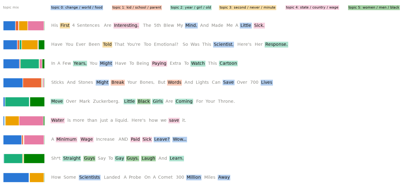
Highlighting makes the mixture idea concrete. "A Minimum Wage Increase AND Paid Sick Leave" is mostly the policy topic, with its "Wow" and "Leave?" from the causes topic. The same word can change topic with the story: "Little" is in topic 0 in the first headline and in topic 2 in "Little Black Girls Are Coming For Your Throne", where the story's mixture favours topic 2. Many words are grey: with a vocabulary of 652 words and headlines of about a dozen words, most of a headline is invisible to the model - one reason these topics are fuzzy.
4. How much of the corpus is each topic, month by month? A topic's prevalence in a month is the average $\theta_{dk}$ over that month's stories. Two sources of uncertainty go into the bands: the mixtures themselves (one line per saved Gibbs sweep) and which stories happened to be tested that month (a Bayesian bootstrap: Dirichlet weights over the month's tests). Small multiples on a shared axis rather than a stacked area chart, so each topic can be read against a straight baseline.
week = uw.groupby("test_id")["test_week"].first().loc[test_ids].to_numpy()
year, wk = week // 100, week % 100
month = (year - year.min()) * 12 + np.minimum((wk - 1) * 12 // 52, 11)      # months since Jan 2013
month_idx, month_codes = pd.factorize(month, sort=True)
month_dates = pd.to_datetime([f"{2013 + m // 12}-{m % 12 + 1:02d}-15" for m in month_codes])
g_prev = np.random.default_rng(9)
prev = np.zeros((theta_txt.shape[1], len(month_codes), K_TXT))
for m in range(len(month_codes)):
    idx = np.flatnonzero(month_idx == m)
    weights = g_prev.dirichlet(np.ones(len(idx)), size=theta_txt.shape[1])      # draw x test
    prev[:, m] = np.einsum("st,stk->sk", weights, theta_txt[0][:, idx])
tests_per_month = np.bincount(month_idx)
print(f"tests per month: min {tests_per_month.min()}, median {np.median(tests_per_month):.0f}, max {tests_per_month.max()}")

fig, axes = plt.subplots(2, 3, figsize=(13, 6), sharex=True, sharey=True)
for k, ax in enumerate(axes.ravel()):
    lo, hi = np.quantile(prev[..., k], [0.05, 0.95], axis=0)
    ax.fill_between(month_dates, lo, hi, color=TOPIC_COLOURS[k], alpha=0.25, lw=0)
    ax.plot(month_dates, prev[..., k].mean(0), color=TOPIC_COLOURS[k], lw=2)
    ax.axhline(1 / K_TXT, color=MUTED, lw=0.8, ls=":")
    ax.set_title(f"topic {k}: {labels_rel[k]}", fontsize=9, loc="left")
    ax.tick_params(axis="x", labelrotation=30, labelsize=8)
fig.supylabel("share of the month's stories", fontsize=10)
fig.suptitle("Topic prevalence by month (90% band; dotted = an even 1/6 share)");
tests per month: min 7, median 156, max 392
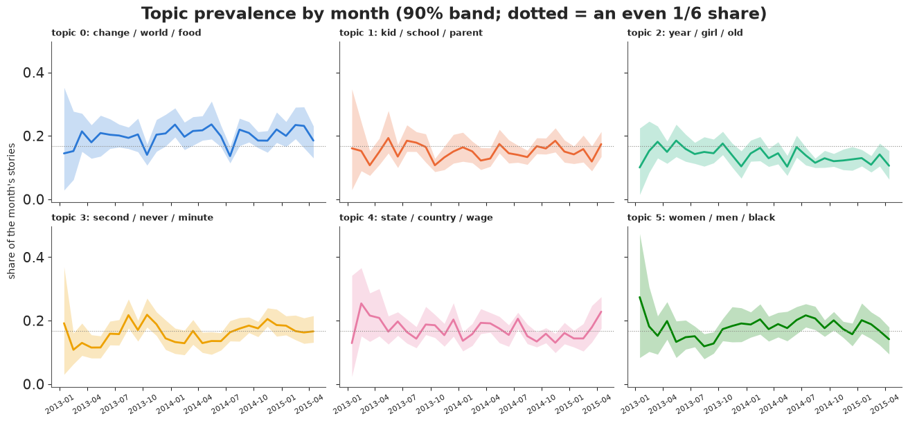
Most topics hold a roughly steady share. Two drift: "women / men / black" goes from about 0.12-0.15 of stories in mid-2013 to about 0.2 through 2014, and "year / girl / old" slides from about 0.15-0.18 in 2013 to about 0.12 in 2015. The first months are wide because they have few tests (7 in the smallest month). Remember that the topics were fitted to the whole period: a topic whose vocabulary changes over time (a dynamic topic model; Blei & Lafferty 2006) is a different model.
C. How many topics, and do topics predict clicks?
The usual answer: held-out likelihood
The textbook way to choose $K$ is document completion: fit on 80% of the tests, then for each held-out test show the model half of its tokens, infer that test's mixture $\theta$ (with the topics fixed), and score the log-probability of the other half. Larger is better. The baseline is a single "topic" (word frequencies of the whole corpus).
@numba.njit
def _foldin_sweeps(doc, word, z, ndk, phi, alpha, n_sweeps, seed):
    np.random.seed(seed)
    K = phi.shape[0]
    cum = np.empty(K)
    for _ in range(n_sweeps):
        for i in range(doc.shape[0]):
            d, w, k = doc[i], word[i], z[i]
            ndk[d, k] -= 1
            total = 0.0
            for j in range(K):
                total += (ndk[d, j] + alpha) * phi[j, w]
                cum[j] = total
            u = np.random.random() * total
            k = 0
            while cum[k] < u:
                k += 1
            z[i] = k
            ndk[d, k] += 1


def completion_score(X_seen, X_hidden, phis, alpha=0.1, sweeps=50, seed=0):
    """Log-probability per hidden token, theta inferred from the seen half, averaged over phi draws."""
    g = np.random.default_rng(seed)
    d_i, w_i = np.nonzero(X_seen)
    n = X_seen[d_i, w_i]
    doc, word = np.repeat(d_i, n), np.repeat(w_i, n)
    K = phis.shape[1]
    prob = np.zeros(X_hidden.shape)
    for s, phi_s in enumerate(phis):
        z = g.integers(K, size=doc.size)
        ndk = np.zeros((X_seen.shape[0], K), np.int64)
        np.add.at(ndk, (doc, z), 1)
        _foldin_sweeps(doc, word, z, ndk, phi_s, alpha, sweeps, seed + s)
        prob += (ndk + alpha) / (ndk.sum(1, keepdims=True) + K * alpha) @ phi_s
    return np.sum(X_hidden * np.log(prob / len(phis))) / X_hidden.sum()


split_rng = np.random.default_rng(1)
is_test = split_rng.random(len(X_txt)) < 0.2
X_train, X_test = X_txt[~is_test], X_txt[is_test]
X_seen = np.zeros_like(X_test)
for d in range(len(X_test)):
    toks = np.repeat(np.arange(len(vocab)), X_test[d])
    split_rng.shuffle(toks)
    np.add.at(X_seen[d], toks[: len(toks) // 2], 1)
X_hidden = X_test - X_seen
unigram = (X_train.sum(0) + 0.5) / (X_train.sum() + 0.5 * len(vocab))
print(f"one-topic baseline: {np.sum(X_hidden * np.log(unigram)) / X_hidden.sum():.3f} nats per token")
one-topic baseline: -6.170 nats per token
The answer that fits the purpose: does it predict clicks?
We want topics for a reason: to learn which kinds of story got clicked. So score each $K$ by how well the topic mixtures predict a test's click-through rate out of sample. Upworthy's click-through moved a lot over these two years (quarterly averages from under 1% to about 3%), so the outcome is the log-odds of click-through minus that month's average (a story is compared with stories of the same month). The score is the 5-fold cross-validated $R^2$ of a ridge regression on the posterior mean mixtures - a quick screen; the model below does it properly. The topic model never sees the clicks, so fitting it on all tests does not leak.
tests = uw.groupby("test_id").agg(clicks=("clicks", "sum"), impressions=("impressions", "sum"),
                                  week=("test_week", "first")).loc[test_ids]
logit_ctr = np.log((tests["clicks"] + 0.5) / (tests["impressions"] - tests["clicks"] + 0.5)).to_numpy()
year, wk = tests["week"].to_numpy() // 100, tests["week"].to_numpy() % 100
month = (year - year.min()) * 12 + np.minimum((wk - 1) * 12 // 52, 11)
month_idx, month_codes = pd.factorize(month, sort=True)
y_rel = logit_ctr - pd.Series(logit_ctr).groupby(month_idx).transform("mean").to_numpy()
cv_fold = np.random.default_rng(2).integers(5, size=len(y_rel))


def cv_r2(F, lam=1.0):
    pred = np.zeros_like(y_rel)
    for f in range(5):
        tr = cv_fold != f
        A = np.c_[np.ones(tr.sum()), F[tr]]
        b = np.linalg.solve(A.T @ A + lam * np.eye(A.shape[1]), A.T @ y_rel[tr])
        pred[~tr] = np.c_[np.ones((~tr).sum()), F[~tr]] @ b
    return 1 - np.mean((y_rel - pred) ** 2) / np.var(y_rel)


rows = []
for K in [2, 4, 6, 10, 20, 40, 80]:
    phi_tr, _, _ = lda_gibbs(X_train, K, burn=500, draws=10, thin=20, seed=K)
    _, theta_all, _ = lda_gibbs(X_txt, K, burn=500, draws=10, thin=20, seed=100 + K)
    rows.append({"K": K, "held-out nats/token": completion_score(X_seen, X_hidden, phi_tr[::2], seed=K),
                 "CV R2 of click-through": cv_r2(theta_all.mean(0))})
choose = pd.DataFrame(rows).set_index("K")
print(choose.round(3))

fig, axes = plt.subplots(1, 2, figsize=(12, 3.6))
axes[0].plot(choose.index, choose.iloc[:, 0], "o-")
axes[0].set(xscale="log", xlabel="number of topics K", ylabel="nats per held-out token",
            title="Held-out words: more topics, always better")
axes[1].plot(choose.index, choose.iloc[:, 1], "o-", color="C1")
axes[1].set(xscale="log", xlabel="number of topics K", ylabel="cross-validated R$^2$",
            title="Click-through: flat from K = 4")
for ax in axes:
    ax.minorticks_off()
    ax.set_xticks(choose.index, choose.index);
    held-out nats/token  CV R2 of click-through
K
2                -6.143                   0.020
4                -6.102                   0.106
6                -6.083                   0.084
10               -6.037                   0.091
20               -5.975                   0.093
40               -5.833                   0.089
80               -5.759                   0.103
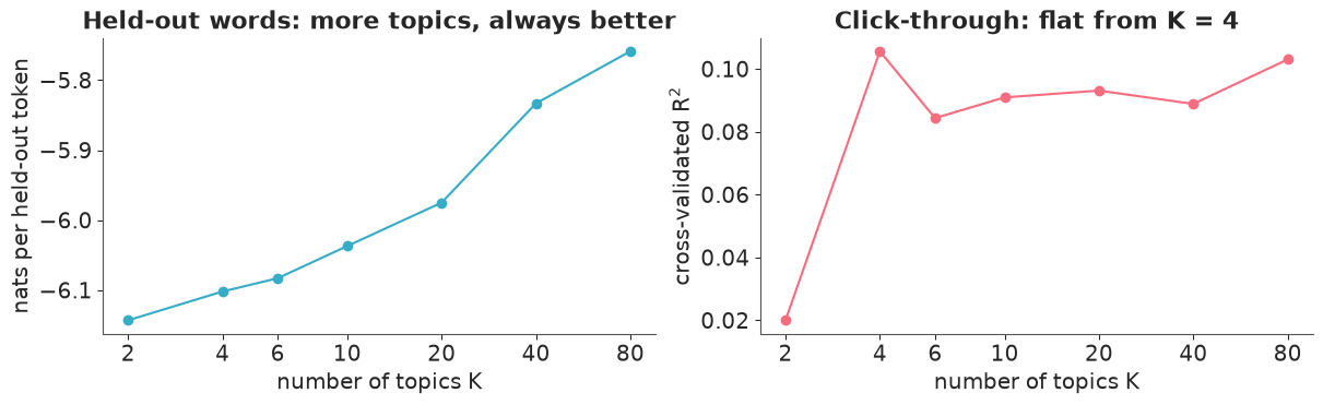
The two criteria disagree. Document completion keeps improving well beyond the point where topics stop being readable: the headlines written for one story repeat that story's words, so the more topics, the closer the model gets to memorising individual stories - an excellent way to predict the other half of a headline set and a poor way to summarise a corpus. (Chang et al. 2009, "Reading tea leaves", found that held-out likelihood and human judgements of topic quality can even move in opposite directions.) The click-through question has a clearer answer: a handful of topics carries what the text says about clickability: two topics explain almost nothing, and from four on the cross-validated $R^2$ stays around 0.08-0.11 with no trend (each $K$ is one LDA run, so differences of 0.02 are noise). We keep $K = 6$ - one of several equally predictive choices, and still readable.
Topics as regressors, with their uncertainty
Now the model. For test $d$ in month $m$, with observed log-odds $y_d$ and its binomial standard error $s_d$ (known from clicks and impressions):
$$y_d \sim \text{Normal}\Big(\mu_{m} + \sum_k \theta_{dk}\,\gamma_k,\; \sqrt{\sigma^2 + s_d^2}\Big), \qquad \mu_m \text{ a Gaussian random walk over months}, \qquad \sum_k \gamma_k = 0.$$
Because every $\boldsymbol\theta_d$ sums to one, an intercept and $K$ free topic effects are not
identified together; a ZeroSumNormal makes each $\gamma_k$ the effect of a story being entirely
about topic $k$ relative to the average topic. $\sigma$ is everything else about a story.
The mixtures $\theta_d$ are estimates, and for a 9-token document they are uncertain. There are two tempting ways to use them:
- plug-in: use each test's posterior mean mixture as if it were known;
- "propagate the uncertainty": fit the regression once for each of several posterior draws of $\theta$ and pool the posterior draws (multiple imputation).
We fit both. The model is compiled once (nutpie) and the data swapped between fits.
import nutpie

se_logit = np.sqrt(1 / (tests["clicks"] + 0.5) + 1 / (tests["impressions"] - tests["clicks"] + 0.5)).to_numpy()
coords_ctr = {"test": np.arange(len(logit_ctr)), "month": month_codes, "topic": labels_txt}
with pm.Model(coords=coords_ctr) as ctr_model:
    theta_data = pm.Data("theta_data", theta_txt[0].mean(0), dims=("test", "topic"))
    y_data = pm.Data("y_data", logit_ctr, dims="test")
    mu_month = pm.GaussianRandomWalk("mu_month", sigma=0.1, init_dist=pm.Normal.dist(-4.0, 1.0),
                                     dims="month")
    gamma = pm.ZeroSumNormal("gamma", sigma=0.5, dims="topic")
    sigma = pm.HalfNormal("sigma", 0.5)
    pm.Normal("y", mu_month[month_idx] + theta_data @ gamma, pt.sqrt(sigma**2 + se_logit**2),
              observed=y_data, dims="test")

compiled_ctr = nutpie.compile_pymc_model(ctr_model)


def fit_gamma(theta_in, y_in, draws=1000, seed=0):
    fit = nutpie.sample(compiled_ctr.with_data(theta_data=theta_in, y_data=y_in), draws=draws, seed=seed,
                        save_warmup=False, progress_bar=False)
    return fit


def plugin_and_imputed(theta_draws, y_in, n_imp=8, seed=0):
    """Posterior draws of gamma: plug-in (posterior-mean mixtures) and pooled over n_imp mixture draws."""
    plug = fit_gamma(theta_draws.mean(0), y_in, seed=seed)
    picks = np.linspace(0, len(theta_draws) - 1, n_imp).astype(int)
    imp = [fit_gamma(theta_draws[p], y_in, draws=250, seed=seed + 1 + i).posterior["gamma"].values.reshape(-1, K_TXT)
           for i, p in enumerate(picks)]
    return plug, plug.posterior["gamma"].values.reshape(-1, K_TXT), np.concatenate(imp)


t0 = time.perf_counter()
fit_plugin, gamma_plugin, gamma_mi = plugin_and_imputed(theta_txt[0], logit_ctr, seed=RANDOM_SEED)
print(f"9 regressions: {time.perf_counter() - t0:.0f} s")
print("plug-in fit: divergences", int(fit_plugin.sample_stats["diverging"].sum()),
      "| max r_hat", round(float(az.rhat(fit_plugin.posterior["gamma"]).max()), 3))
print(pd.DataFrame({"plug-in mean": gamma_plugin.mean(0), "plug-in sd": gamma_plugin.std(0),
                    "imputed mean": gamma_mi.mean(0), "imputed sd": gamma_mi.std(0)},
                   index=labels_txt).round(3))
9 regressions: 4 s
plug-in fit: divergences 0 | max r_hat 1.003
                        plug-in mean  plug-in sd  imputed mean  imputed sd
world / video / change        -0.420       0.028        -0.284       0.028
kid / school / parent          0.027       0.032         0.010       0.030
year / girl / old              0.443       0.033         0.331       0.033
never / video / minute         0.207       0.031         0.125       0.028
state / reason / time         -0.449       0.030        -0.318       0.033
women / guy / men              0.192       0.029         0.136       0.026
The two disagree, and not in the way "propagating uncertainty" suggests: the imputed effects are not just wider, they are about a third smaller. Which is right? Ask a simulation where we know the answer. Take the fitted topics and one posterior draw of the mixtures as the truth, generate a fake corpus with the real document lengths, generate fake click-through log-odds with known effects $\gamma$ (the plug-in estimates), refit LDA to the fake corpus, align its topics to the true ones, and run both regressions.
sim_rng = np.random.default_rng(7)
phi_truth, theta_truth = phi_txt[0].mean(0), theta_txt[0, -1]
gamma_truth = gamma_plugin.mean(0)
mu_hat = fit_plugin.posterior["mu_month"].mean(("chain", "draw")).values
sigma_hat = float(fit_plugin.posterior["sigma"].mean())
X_fake = np.array([sim_rng.multinomial(n, p) for n, p in zip(X_txt.sum(1), theta_truth @ phi_truth)])
y_fake = (mu_hat[month_idx] + theta_truth @ gamma_truth
          + sim_rng.normal(0, np.sqrt(sigma_hat**2 + se_logit**2)))
phi_f, theta_f, _ = lda_gibbs(X_fake, K_TXT, seed=11)
perm_f = align_to(phi_truth, phi_f.mean(0))
theta_f = theta_f[..., perm_f]
print("cosine of refitted topics to the true ones:", np.round(cosine(phi_truth, phi_f.mean(0)[perm_f]), 2))
_, g_plug_f, g_mi_f = plugin_and_imputed(theta_f, y_fake, seed=21)
_, g_true_f, _ = plugin_and_imputed(theta_truth[None], y_fake, n_imp=1, seed=31)
sim_tab = pd.DataFrame({"true gamma": gamma_truth, "true mixtures known": g_true_f.mean(0),
                        "plug-in": g_plug_f.mean(0), "imputed": g_mi_f.mean(0)}, index=labels_txt)
print(sim_tab.round(3))
slope = lambda est: np.sum(est * gamma_truth) / np.sum(gamma_truth**2)
print(f"estimate / truth (least-squares slope): plug-in {slope(g_plug_f.mean(0)):.2f}, "
      f"imputed {slope(g_mi_f.mean(0)):.2f}")
cosine of refitted topics to the true ones: [0.99 0.99 0.99 0.98 0.98 0.99]
                        true gamma  true mixtures known  plug-in  imputed
world / video / change      -0.420               -0.445   -0.419   -0.318
kid / school / parent        0.027                0.005    0.027    0.028
year / girl / old            0.443                0.460    0.431    0.332
never / video / minute       0.207                0.209    0.175    0.125
state / reason / time       -0.449               -0.465   -0.456   -0.355
women / guy / men            0.192                0.236    0.241    0.187
estimate / truth (least-squares slope): plug-in 1.00, imputed 0.77
The simulation settles it. With the true mixtures, the regression recovers the true effects (up to noise); with plug-in posterior means it still does (slope 1.00 against the truth); pooling over posterior draws shrinks every effect by about a quarter (0.77). The same shrinkage as on the real data.
Why: a single posterior draw of $\theta_d$ is the posterior mean plus noise that knows nothing about clicks. Noise added to a regressor is classical measurement error, and it attenuates slopes. The posterior mean has the other kind of error: truth = estimate + noise independent of the estimate (Berkson error), which leaves a linear regression's slope unbiased - this is "regression calibration". The general rule behind it: multiple imputation is valid only when the imputation model includes the outcome, and a topic model's posterior knows nothing about clicks. The fully Bayesian alternative is one joint model in which clicks and words both inform the mixtures - supervised LDA (Blei & McAuliffe 2007) - at a much higher computational cost.
A second lesson hides in the first line of output: on fake data drawn from LDA, a single chain finds the true topics almost exactly (cosine 0.98-0.99). The instability of part B is therefore not a sampler failure - it is what happens when real headlines are not generated by LDA and several different six-topic summaries fit them about equally well.
So we report the plug-in effects. The plug-in standard deviations ignore the uncertainty in the mixtures and are somewhat too small; with sd around 0.03 against effects of 0.2-0.45 that does not change any conclusion here.
eff = pd.DataFrame({"effect on log-odds": gamma_plugin.mean(0), "sd": gamma_plugin.std(0),
                    "P(effect > 0)": (gamma_plugin > 0).mean(0),
                    "odds vs average story": np.exp(gamma_plugin).mean(0)}, index=labels_txt)
print(eff.round(3))
print("sigma (story-to-story sd of log-odds):", round(float(fit_plugin.posterior["sigma"].mean()), 3))

order = np.argsort(gamma_plugin.mean(0))
fig, ax = plt.subplots(figsize=(8, 3.8))
for j, (g_draws, name, off) in enumerate([(gamma_plugin, "plug-in: posterior-mean mixtures", 0.12),
                                           (gamma_mi, "pooled over mixture draws (attenuated)", -0.12)]):
    lo, hi = np.quantile(np.exp(g_draws), [0.05, 0.95], axis=0)
    mid = np.exp(g_draws).mean(0)
    ax.errorbar(mid[order], np.arange(K_TXT) + off, xerr=[mid[order] - lo[order], hi[order] - mid[order]],
                fmt="o", color=f"C{j}", alpha=1 if j == 0 else 0.45, label=name)
ax.axvline(1, color="k", lw=0.8)
ax.set_yticks(range(K_TXT), np.array(labels_txt)[order])
ax.set(xlabel="click-through odds for a story entirely about the topic, vs an average story (90% interval)",
       title="Which kinds of Upworthy story got clicked (same month)")
ax.legend(fontsize=8, loc="lower right");
                        effect on log-odds     sd  P(effect > 0)  odds vs average story
world / video / change              -0.420  0.028          0.000                  0.657
kid / school / parent                0.027  0.032          0.805                  1.028
year / girl / old                    0.443  0.033          1.000                  1.558
never / video / minute               0.207  0.031          1.000                  1.230
state / reason / time               -0.449  0.030          0.000                  0.639
women / guy / men                    0.192  0.029          1.000                  1.213
sigma (story-to-story sd of log-odds): 0.545
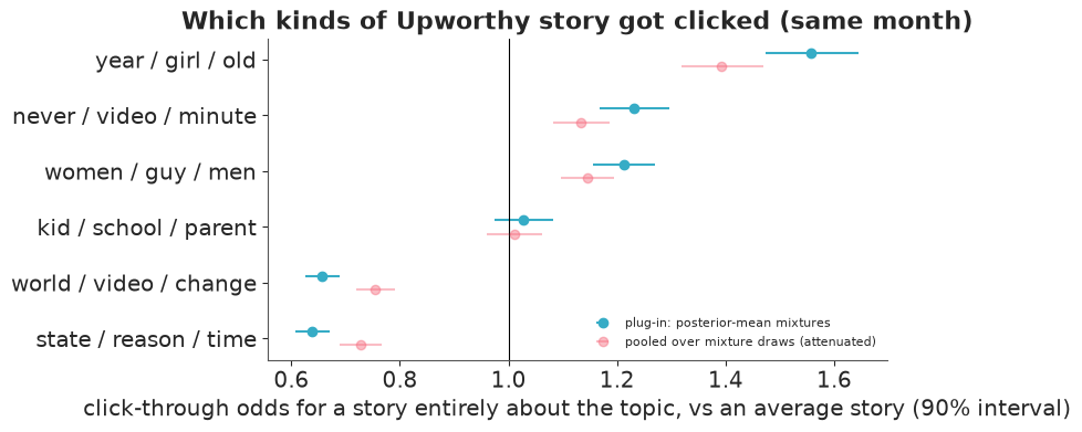
Stories about the "year / girl / old" topic (a child or a person introduced by age, and questions asked and answered - "gay" and "ask" are in it too) had about 1.5 times the click-through odds of an average story of the same month; "never / video / minute" (watch-this-video stories) and "women / guy / men" (gender, and race: "black", "white" are in it) about 1.2 times. Stories about "state / reason / time" (America, jobs, money: policy) and "world / video / change" (big causes: food, change, the world) had about two thirds of the average odds. "kid / school / parent" is indistinguishable from average. The story-to-story sd of log-odds that topics do not explain is 0.55 - topics are a small part of what made a story clickable. Topics are fuzzy (part B), so read these as descriptions of how stories clustered, not as a lever: nothing here says that rewriting a policy story as a family story would earn more clicks. That is a causal question, and the headline experiments in E66 answer the version of it that can be answered (wording, within a story).
D. From posters to documents: a colour vocabulary
Now the same model on pictures. The collection: 750 public-domain posters from the Library of Congress, 250 from each of three moments in the history of printed advertising and persuasion:
- 1890s magazine posters - the American "poster craze", when magazines (Harper's, The Century, Scribner's, Lippincott's, The Chap-Book) commissioned artists such as Edward Penfield and Will Bradley to sell each month's issue;
- First World War posters (1914-1919) - recruitment, war loans, food conservation, relief;
- WPA posters (1936-1943) - the New Deal's Federal Art Project: health campaigns, theatre, travel, exhibitions, in silkscreen.
data.describe("loc_posters_thumbs")
posters = np.load(data.path("loc_posters_thumbs"))
thumbs, era, poster_year, poster_title = posters["thumbs"], posters["era"], posters["year"], posters["title"]
ERAS = ["1890s magazine", "WWI", "WPA"]
era_idx = np.array([ERAS.index(e) for e in era])
print(thumbs.shape, dict(zip(*np.unique(era, return_counts=True))))

fig, axes = plt.subplots(3, 16, figsize=(13, 3.6))
for r, e in enumerate(ERAS):
    for c, i in enumerate(np.flatnonzero(era_idx == r)[:16]):
        axes[r, c].imshow(thumbs[i])
        axes[r, c].axis("off")
    axes[r, 0].set_title(e, fontsize=9, loc="left")
fig.suptitle("The first 16 posters of each era, as stored (64 x 48 pixels)");
loc_posters_thumbs: NumPy .npz (open data.path(...) with np.load): thumbs (750 x 64 x 48 x 3 uint8 RGB, rows = height), era ('1890s magazine', 'WWI', 'WPA'; 250 each), year (first four-digit year in the LoC date), title, creator, loc_id, image_url. Many scans include the black or grey backing and a colour-checker strip around the poster (most often in the WWI group).
  source: Library of Congress Prints & Photographs Division: Posters collection (search 'magazine', dated 1889-1905; search 'world war 1914-1918', dated 1914-1919) and Work Projects Administration Poster Collection (co=wpapos, dated 1935-1943); public domain / no known restrictions on publication per the LoC rights statements. BUILT by tools/fetch_loc_posters.py (seed 72): 250 randomly sampled items per era with a dated year and a reference image; each 640-px reference JPEG (the URL's `image.full`) resized to 64 x 48 with Lanczos. Keep the cached file in data/ (a rebuild draws from whatever the live search returns).
  url:    https://www.loc.gov/pictures/search/?co=pos&fo=json
(750, 64, 48, 3) {np.str_('1890s magazine'): np.int64(250), np.str_('WPA'): np.int64(250), np.str_('WWI'): np.int64(250)}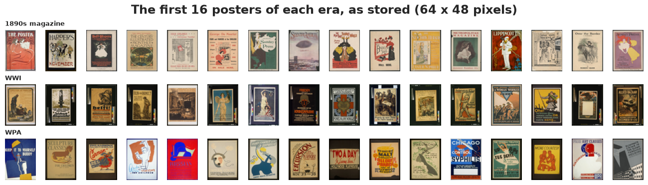
Look at the WWI row: many scans show the poster on a black backing, with a colour-checker strip beside it. A topic model would learn "black scan background" as a palette - and since it is far more common in one era, it would also look like an era effect. What the measurement pipeline adds to every document of one kind is the pictorial version of boilerplate text (copyright lines, e-mail footers), and it has to go before modelling. We estimate the backing colour from the four corners and keep the rows and columns in which most pixels differ from it (a crude crop: posters that are themselves dark at the edges keep their border).
Then the vocabulary. Colours are compared in CIELab, a colour space designed so that Euclidean distance roughly matches perceived difference (RGB is not). A codebook of 32 colours is learned by k-means on a sample of pixels from all posters; each pixel becomes the index of its nearest code colour - its "word". This is the "bag of visual words" idea from computer vision, with colours as the simplest possible visual words (patches, textures or features from a neural network work the same way).
M_XYZ = np.array([[0.4124, 0.3576, 0.1805], [0.2126, 0.7152, 0.0722], [0.0193, 0.1192, 0.9505]])
WHITE = np.array([0.95047, 1.0, 1.08883])


def rgb_to_lab(rgb):
    c = np.asarray(rgb, float) / 255
    c = np.where(c > 0.04045, ((c + 0.055) / 1.055) ** 2.4, c / 12.92)
    f = c @ M_XYZ.T / WHITE
    f = np.where(f > (6 / 29) ** 3, np.cbrt(f), f / (3 * (6 / 29) ** 2) + 4 / 29)
    return np.stack([116 * f[..., 1] - 16, 500 * (f[..., 0] - f[..., 1]), 200 * (f[..., 1] - f[..., 2])], -1)


def lab_to_rgb(lab):
    fy = (lab[..., 0] + 16) / 116
    f = np.stack([fy + lab[..., 1] / 500, fy, fy - lab[..., 2] / 200], -1)
    xyz = np.where(f > 6 / 29, f**3, 3 * (6 / 29) ** 2 * (f - 4 / 29)) * WHITE
    c = np.clip(xyz @ np.linalg.inv(M_XYZ).T, 0, 1)
    return np.clip(np.where(c > 0.0031308, 1.055 * c ** (1 / 2.4) - 0.055, 12.92 * c), 0, 1)


def crop_box(img, threshold=12.0, frac=0.6):
    """Rows/columns where most pixels differ (Delta E > threshold) from the median corner colour."""
    lab = rgb_to_lab(img)
    corners = np.concatenate([lab[:3, :3], lab[:3, -3:], lab[-3:, :3], lab[-3:, -3:]]).reshape(-1, 3)
    fg = np.linalg.norm(lab - np.median(corners, 0), axis=-1) > threshold
    rows, cols = np.flatnonzero(fg.mean(1) > frac), np.flatnonzero(fg.mean(0) > frac)
    if len(rows) < 16 or len(cols) < 12:          # nothing clearly separable: keep the whole image
        return 0, img.shape[0], 0, img.shape[1]
    return rows[0] + 1, rows[-1], cols[0] + 1, cols[-1]   # one more pixel in, for resampling halos


def nearest(lab_pixels, codebook, chunk=100_000):
    out = np.empty(len(lab_pixels), np.int64)
    for s in range(0, len(lab_pixels), chunk):   # chunks: a pixels x codebook x 3 array gets big
        d2 = ((lab_pixels[s:s + chunk, None, :] - codebook[None]) ** 2).sum(-1)
        out[s:s + chunk] = d2.argmin(1)
    return out


def kmeans(x, k, g, iters=50):
    centres = [x[g.integers(len(x))]]
    for _ in range(k - 1):                        # k-means++ seeding
        d2 = ((x[:, None] - np.array(centres)[None]) ** 2).sum(-1).min(1)
        centres.append(x[g.choice(len(x), p=d2 / d2.sum())])
    centres = np.array(centres)
    for _ in range(iters):
        lab = nearest(x, centres)
        centres = np.array([x[lab == j].mean(0) if np.any(lab == j) else centres[j] for j in range(k)])
    return centres


boxes = np.array([crop_box(t) for t in thumbs])
kept_share = (boxes[:, 1] - boxes[:, 0]) * (boxes[:, 3] - boxes[:, 2]) / (64 * 48)
print("share of the thumbnail kept, median by era:",
      {e: round(float(np.median(kept_share[era_idx == i])), 2) for i, e in enumerate(ERAS)})
poster_lab = [rgb_to_lab(t[r0:r1, c0:c1]).reshape(-1, 3) for t, (r0, r1, c0, c1) in zip(thumbs, boxes)]

V_COL = 32
g_col = np.random.default_rng(3)
pixel_sample = np.concatenate([p[g_col.choice(len(p), 60, replace=False)] for p in poster_lab])
codebook = kmeans(pixel_sample, V_COL, g_col)
chroma, hue = np.hypot(codebook[:, 1], codebook[:, 2]), np.arctan2(codebook[:, 2], codebook[:, 1])
codebook = codebook[np.lexsort((codebook[:, 0], np.where(chroma < 12, -10, np.round(hue * 2))))]  # greys, then by hue
swatch = lab_to_rgb(codebook)
chroma, hue = np.hypot(codebook[:, 1], codebook[:, 2]), np.arctan2(codebook[:, 2], codebook[:, 1])
poster_words = [nearest(p, codebook) for p in poster_lab]

# For display, colours are grouped into families: the chromatic ones in hue order (red, orange,
# yellow, green, blue), then the earth tones and neutrals that dominate old paper (beige/tan,
# brown, grey), sorted light to dark within a family. CIELab hue alone would call every beige and
# brown "yellow" (they sit at hue angles of 70-95 degrees), so lightness and chroma split them off.
FAMILIES = ["red", "orange", "yellow", "green", "blue", "beige", "brown", "grey"]
hue_deg = np.degrees(hue) % 360
code_family = np.select(
    [chroma < 13,                                            # grey: too little colour to have a hue
     (hue_deg >= 105) & (hue_deg < 200),                     # green
     hue_deg >= 200,                                         # blue (no violets in this vocabulary)
     (hue_deg < 55) & (chroma >= 22) & (codebook[:, 0] < 58),  # red, brick, maroon
     (chroma >= 40) & (hue_deg < 75),                        # orange
     chroma >= 40,                                           # yellow: gold and ochre
     codebook[:, 0] < 50],                                   # brown: dark, muted warm
    [7, 3, 4, 0, 1, 2, 6], 5)                                # otherwise beige / tan
print({f: ", ".join(map(str, np.flatnonzero(code_family == i))) for i, f in enumerate(FAMILIES)})
display_order = np.lexsort((-codebook[:, 0], code_family))


def palette_squares(ax, weights, labels=True, min_label=0.1):
    """A colour distribution as a unit square: one column per colour family (width = the family's
    share; chromatic families in hue order, then beige, brown, grey), its colours stacked light (top)
    to dark (height = share within the family). Every rectangle's area is the colour's share."""
    w = np.asarray(weights, float) / np.sum(weights)
    x = 0.0
    for f in range(len(FAMILIES)):
        members = display_order[code_family[display_order] == f]
        total = w[members].sum()
        if total < 1e-4:
            continue
        y = 1.0
        for j in members:
            h = w[j] / total
            ax.add_patch(plt.Rectangle((x, y - h), total, h, facecolor=swatch[j], edgecolor="white", lw=0.6))
            y -= h
        if labels and total >= min_label:
            ax.text(x + total / 2, -0.02, FAMILIES[f], ha="center", va="top", fontsize=7, color="0.3")
        x += total
    ax.set(xlim=(0, 1), ylim=(0, 1), aspect="equal")
    ax.axis("off")


share_all = np.bincount(np.concatenate(poster_words), minlength=V_COL) / sum(map(len, poster_words))
fig = plt.figure(figsize=(12, 3.4))
left, right = fig.subfigures(1, 2, width_ratios=[2.6, 1])
axes = left.subplots(2, 1, height_ratios=[1, 1.4])
axes[0].imshow(swatch[display_order][None], aspect="auto")
axes[0].set(yticks=[])
axes[0].set_title("The colour vocabulary: 32 k-means colours by family, light to dark", fontsize=10)
fam_sorted = code_family[display_order]
starts = [np.flatnonzero(fam_sorted == f) for f in range(len(FAMILIES))]
axes[0].set_xticks([s_.mean() for s_ in starts if len(s_)], [FAMILIES[f] for f, s_ in enumerate(starts) if len(s_)],
                   fontsize=8)
for s_ in starts[1:]:
    if len(s_):
        axes[0].axvline(s_[0] - 0.5, color="white", lw=2)
axes[1].bar(range(V_COL), share_all[display_order], color=swatch[display_order], edgecolor="0.4", lw=0.4)
axes[1].set(xlim=(-0.5, V_COL - 0.5), xticks=[], ylabel="share of pixels")
palette_squares(right.subplots(), share_all, min_label=0.05)
right.suptitle("All 750 posters, as areas", fontsize=10);
share of the thumbnail kept, median by era: {'1890s magazine': 0.88, 'WWI': 0.71, 'WPA': 0.81}{'red': '13, 14, 15, 16', 'orange': '18', 'yellow': '22, 26, 27', 'green': '31', 'blue': '8, 9, 10, 11, 12', 'beige': '17, 23, 25, 28, 29, 30', 'brown': '19, 20, 21', 'grey': '0, 1, 2, 3, 4, 5, 6, 7, 24'}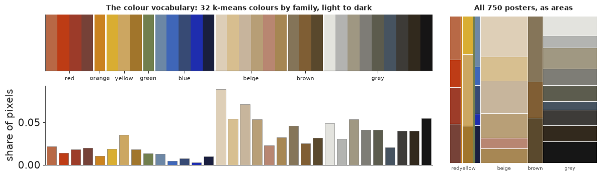
Reading the square charts. From here on, any colour distribution - a poster, a palette, an era - is drawn as a square in which every rectangle's area is a colour's share. Columns are colour families (red, orange, yellow, green, blue, then beige, brown and grey), always in that order, with widths equal to the family's share; within a column the colours are stacked light to dark. Because the order never changes, two squares can be compared position by position: a wide grey column on the right, a thin red sliver on the left. (A strip or a pie ranks colours by weight and loses this.)
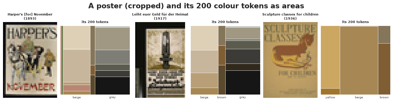
Each poster is now a document of colour words. How many tokens should a crop of about 2,600 pixels contribute? LDA's multinomial treats tokens as independent draws, but neighbouring pixels are nearly copies of each other, so 2,600 pixels carry far less than 2,600 independent pieces of evidence. We take 200 randomly chosen pixels per poster as its tokens (equal length for every document), and part G checks what that choice does.
N_TOK = 200
X_col = np.array([np.bincount(w[g_col.choice(len(w), N_TOK, replace=False)], minlength=V_COL)
                  for w in poster_words])

fig, axes = plt.subplots(1, 6, figsize=(13, 3.3), width_ratios=[1, 1.25] * 3)
for c, i in enumerate([np.flatnonzero(era_idx == r)[1] for r in range(3)]):
    r0, r1, c0, c1 = boxes[i]
    axes[2 * c].imshow(thumbs[i][r0:r1, c0:c1])
    axes[2 * c].axis("off")
    axes[2 * c].set_title(f"{poster_title[i][:30]}\n({poster_year[i]})", fontsize=8)
    palette_squares(axes[2 * c + 1], X_col[i])
    axes[2 * c + 1].set_title("its 200 tokens", fontsize=8)
fig.suptitle("A poster (cropped) and its 200 colour tokens as areas");
E. Palette topics
The corpus is small in vocabulary (32) and long in documents (200 tokens), the opposite of the headlines. We fit $K = 6$ palettes. The PyMC model of part A runs here, but slowly: while preparing the notebook it needed ~3 minutes with the maximum tree depth on almost every transition, and its four chains agreed on only some of the palettes. The collapsed Gibbs sampler of part B takes about two seconds per run, so we run it from 8 random starts and compare: the restart with the highest likelihood is our palette set, and the agreement between restarts says which palettes are robust.
K_COL = 6
t0 = time.perf_counter()
col_runs = [lda_gibbs(X_col, K_COL, alpha=0.5, beta=0.5, burn=1000, draws=20, thin=10, seed=s) for s in range(8)]
print(f"8 restarts: {time.perf_counter() - t0:.0f} s")
col_ll = np.array([r[2].mean() for r in col_runs])
best = int(np.argmax(col_ll))
print("mean token log-likelihood per restart:", np.round(col_ll - col_ll.max()), "(best = 0)")

phi_col_draws = col_runs[best][0]
phi_col = phi_col_draws.mean(0)
theta_col = col_runs[best][1].mean(0)
# order palettes by how much of the corpus they explain
pal_order = np.argsort(-theta_col.mean(0))
phi_col_draws, phi_col, theta_col = phi_col_draws[:, pal_order], phi_col[pal_order], theta_col[:, pal_order]
match = []
for s, r in enumerate(col_runs):
    other = r[0].mean(0)
    perm = linear_sum_assignment(-cosine(phi_col[:, None], other[None]))[1]
    match.append(cosine(phi_col, other[perm]))
match = np.array(match)
print("palette similarity to its best match in each restart (min / median):")
print(pd.DataFrame({"min": match.min(0), "median": np.median(match, 0)},
                   index=[f"palette {k}" for k in range(K_COL)]).round(2).T)
8 restarts: 18 s
mean token log-likelihood per restart: [-9741. -1415.  -574.   -23. -1064.  -980. -2570.     0.] (best = 0)
palette similarity to its best match in each restart (min / median):
        palette 0  palette 1  palette 2  palette 3  palette 4  palette 5
min          0.96       0.16       0.71       0.16       0.41       0.68
median       1.00       0.96       0.99       0.96       0.83       1.00
def palette_bar(ax, weights, lw=0):
o = display_order
ax.barh(0, weights[o], left=np.r_[0, np.cumsum(weights[o])[:-1]], color=swatch[o], edgecolor="none", height=1)
ax.set(xlim=(0, 1), ylim=(-0.5, 0.5))
ax.axis("off")
fig = plt.figure(figsize=(12, 12.5))
sub = fig.subfigures(K_COL, 1)
for k in range(K_COL):
axes = sub[k].subplots(1, 9, width_ratios=[1.5, 0.25] + [1] * 7)
palette_squares(axes[0], phi_col[k])
sub[k].suptitle(f"palette {k}: {theta_col[:, k].mean():.0%} of pixels, "
f"similarity in restarts >= {match[:, k].min():.2f}", fontsize=9, x=0.01, ha="left")
axes[1].axis("off")
for ax, i in zip(axes[2:], np.argsort(-theta_col[:, k])[:7]):
r0, r1, c0, c1 = boxes[i]
ax.imshow(thumbs[i][r0:r1, c0:c1])
ax.set_title(f"{era[i][:5]} {theta_col[i, k]:.2f}", fontsize=6)
ax.axis("off")
fig.suptitle("Six palette topics (left: colour shares as areas, by colour family) and the posters most made of each (right)")
print("largest posterior sd of any colour share in any palette:", round(float(phi_col_draws.std(0).max()), 4));
largest posterior sd of any colour share in any palette: 0.0047
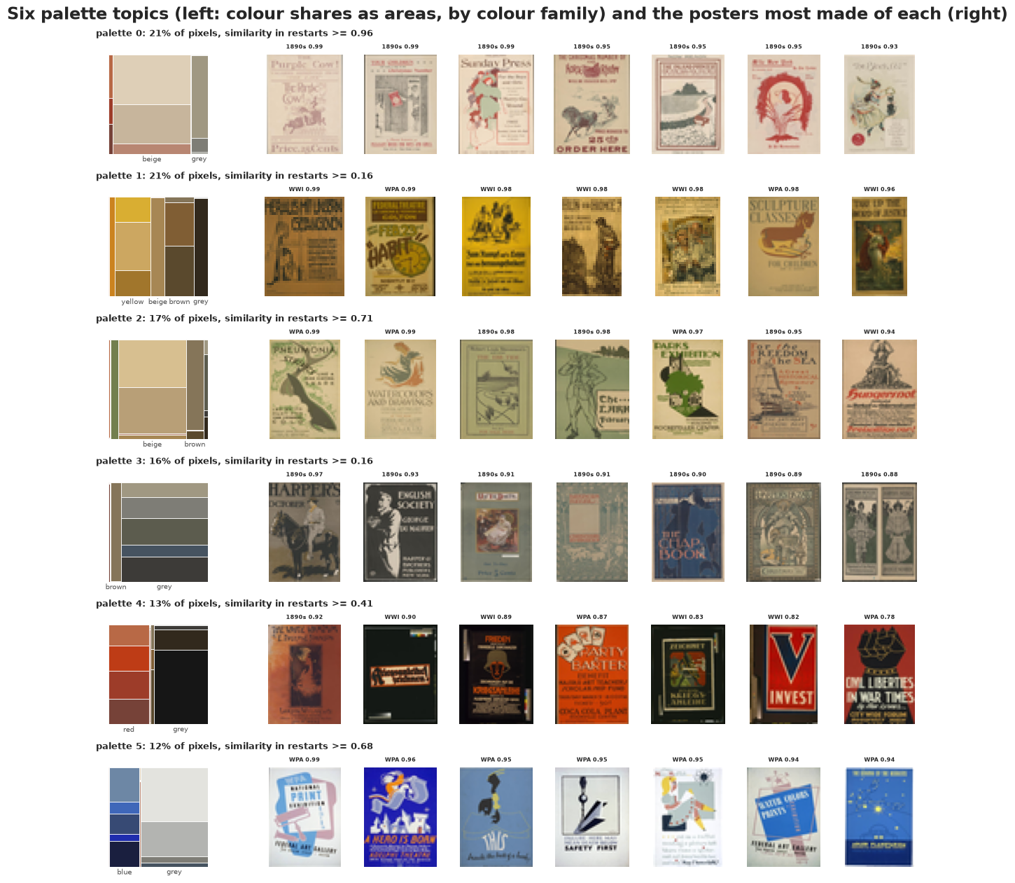
Six palettes, each with a clear visual identity, and none of them was told anything about eras:
- palette 0, cream and beige with a little brick red: aged uncoated paper with sparse printing - almost only 1890s magazine posters. Found in every restart (similarity >= 0.96).
- palette 1, ochre, gold and dark brown: the warm, dark lithographs of WWI and some WPA silkscreens (and old varnish-yellowed paper).
- palette 2, tan with olive green: mixed eras.
- palette 3, greys and slate blue: mostly 1890s posters printed in one or two inks.
- palette 4, black with reds: the dark backgrounds of WWI posters (and leftover black scan backing) and the bold red-and-black graphics of the late 1930s ("Invest", "Civil liberties").
- palette 5, white, greys and blues: WPA silkscreen posters on bright white paper.
Palette 0 is the pictorial "stopword": it is mostly the paper, not a design choice, and it carries an era signal because 130-year-old paper yellows. In a study of design choices you would want to model the substrate separately, just as text models drop boilerplate. Palettes 1 and 3 are not found in every restart (min similarity 0.16), though they are in most (median 0.96): some restarts split the dark colours differently.
The posterior uncertainty within this solution is tiny: with 150,000 tokens the largest posterior sd of any colour share is below 0.005. As with the headlines, the honest uncertainty about palettes is between solutions, not within one.
Better ways to look at palettes
A palette strip shows which colours a topic uses and how much, but not how they relate: light against dark, warm against cool, muted against saturated. And a list of "posters most made of this palette" shows the extreme posters, not what the model does with a typical one that mixes palettes. Four displays.
1. Palettes on a colour map. Each code colour sits at its hue (left to right) and its lightness (bottom = dark, top = light); near-neutral colours (chroma below 12) get their own column on the left, since grey has no hue. Circle area is the colour's weight in the palette, and the faint dots are the rest of the vocabulary for reference. Each palette is identified by the small coloured square in its title - the same identity colour is used in the next two figures.
PALETTE_IDS = TOPIC_COLOURS                           # identity colours for palettes 0-5 (same fixed order)
hue_deg = np.degrees(np.arctan2(codebook[:, 2], codebook[:, 1])) % 360
neutral = chroma < 12
# hue axis: keep 0-140 degrees (reds to greens, where most of these colours are) and squeeze the
# nearly empty 140-360 range (cyan to violet) into 70 units
def hue_axis(h):
    return np.where(h <= 140, h, 140 + (h - 140) * 70 / 220)


x_code = np.where(neutral, -40, hue_axis(hue_deg))
lightness = codebook[:, 0]

fig, axes = plt.subplots(2, 3, figsize=(13, 7.5), sharex=True, sharey=True)
for k, ax in enumerate(axes.ravel()):
    ax.scatter(x_code, lightness, s=10, color=swatch, alpha=0.35, lw=0)
    ax.scatter(x_code, lightness, s=phi_col[k] * 4000, color=swatch, edgecolor="0.25", lw=0.6, zorder=3)
    ax.axvspan(-60, -20, color="0.94", zorder=0, lw=0)
    ax.plot([0.0], [1.06], "s", ms=10, color=PALETTE_IDS[k], transform=ax.transAxes, clip_on=False)
    ax.set_title(f"      palette {k}  ({theta_col[:, k].mean():.0%} of pixels)", fontsize=9, loc="left")
    ax.set(xlim=(-60, 215), ylim=(5, 100))
for ax in axes[1]:
    ticks = {"neutral": -40, "red": 25, "orange": 60, "yellow": 95, "green": 130,
             "blue-violet": float(hue_axis(270))}
    ax.set_xticks(list(ticks.values()), list(ticks.keys()), fontsize=8)
axes[1, 1].set_xlabel("hue (cyan to violet compressed)")
for ax in axes[:, 0]:
    ax.set_ylabel("lightness L*")
fig.suptitle("Where each palette sits in colour space (circle area = weight of the colour in the palette)");
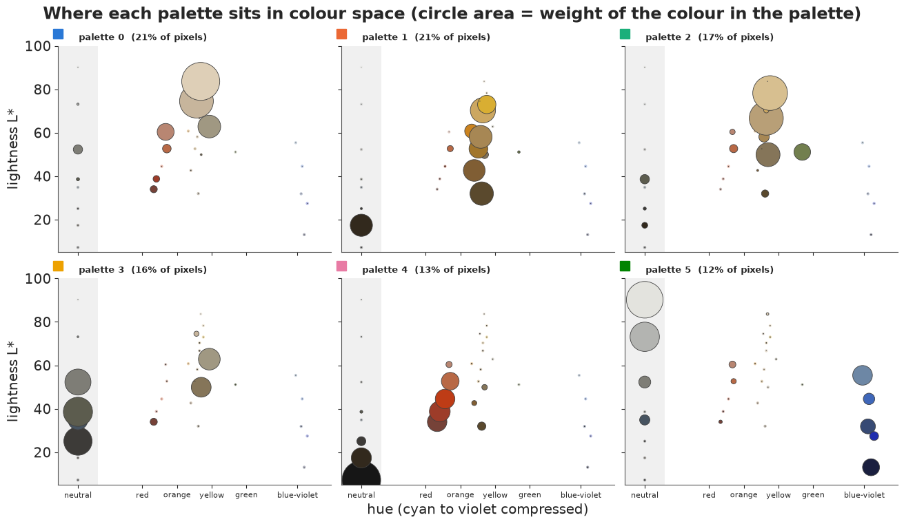
The map separates palettes that look alike as strips. Palettes 0 and 2 are both light and warm, but palette 0 is light neutrals and pinkish beige (paper) while palette 2 adds a mid-tone olive green and a darker tan. Palette 1 is a column of ochres and golds at every lightness. Palette 3 is dark neutrals with one slate blue, palette 4 near-black with the saturated reds, and palette 5 the only light palette with real blues - the white paper and printed blues of the silkscreens.
2. One poster through the model's eyes. For a poster with mixture $\theta_d$, each pixel's colour word $w$ belongs to palette $k$ with probability $\propto \theta_{dk}\,\phi_{kw}$. Painting every pixel with the identity colour of its most probable palette turns the model into a segmentation: which part of the poster is "paper", which is "ink", which is "sky". Below each poster, a posterior predictive check in colour: its actual colour distribution (all pixels) against the model's, $\boldsymbol\theta_d^\top\Phi$. Two posters from each era that mix at least two palettes.
mixing = np.flatnonzero(np.sort(theta_col, 1)[:, -2] > 0.25)
g_show = np.random.default_rng(10)
picks = np.concatenate([g_show.choice(mixing[era_idx[mixing] == e], 2, replace=False) for e in range(3)])
id_rgb = np.array([plt.matplotlib.colors.to_rgb(c) for c in PALETTE_IDS])

fig = plt.figure(figsize=(13, 10))
top_fig, legend_fig = fig.subfigures(2, 1, height_ratios=[8, 1.8])
grid = top_fig.subplots(3, len(picks), height_ratios=[3, 3, 1.3])
tv_dist = []
for c, i in enumerate(picks):
    r0, r1, c0, c1 = boxes[i]
    words_i = poster_words[i]
    resp = theta_col[i][:, None] * phi_col[:, words_i]              # palette x pixel
    seg = id_rgb[resp.argmax(0)].reshape(r1 - r0, c1 - c0, 3)
    grid[0, c].imshow(thumbs[i][r0:r1, c0:c1])
    grid[0, c].set_title(f"{poster_title[i][:24]}\n{poster_year[i]}, {ERAS[era_idx[i]]}", fontsize=7)
    grid[1, c].imshow(seg)
    observed = np.bincount(words_i, minlength=V_COL) / len(words_i)
    fitted = theta_col[i] @ phi_col
    tv_dist.append(0.5 * np.abs(observed - fitted).sum())
    grid[2, c].axis("off")
    for pos, dist, name in [(0.0, observed, "actual"), (0.52, fitted, "model")]:
        ins = grid[2, c].inset_axes([pos, 0, 0.48, 1])
        palette_squares(ins, dist, labels=False)
        ins.set_title(name, fontsize=7, pad=2)
    for ax in grid[:2, c]:
        ax.axis("off")
top_fig.suptitle("Posters (top), each pixel's most probable palette (middle), actual vs model colours as areas (bottom)")
leg = legend_fig.subplots(1, K_COL)
for k, ax in enumerate(leg):
    palette_squares(ax, phi_col[k], labels=False)
    ax.set_title(f"palette {k}", fontsize=8, color=INK)
    ax.plot([-0.12], [0.5], "s", ms=11, color=PALETTE_IDS[k], transform=ax.transAxes, clip_on=False)
print("total-variation distance, actual vs model colours:", np.round(tv_dist, 2))
tv_all = np.array([0.5 * np.abs(np.bincount(w, minlength=V_COL) / len(w) - theta_col[i] @ phi_col).sum()
                   for i, w in enumerate(poster_words)])
print(f"all 750 posters: median {np.median(tv_all):.2f}, 90th percentile {np.percentile(tv_all, 90):.2f}")
total-variation distance, actual vs model colours: [0.36 0.4  0.2  0.34 0.62 0.39]
all 750 posters: median 0.39, 90th percentile 0.54
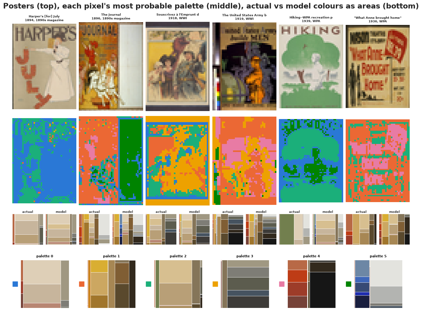
The segmentations read like a printer's separation. "Harper's July" (1894) is paper (palette 0) plus figure and lettering (palette 2). The WPA "Hiking" poster puts its trees in palette 2 (the olive green) and its ground in palette 0. In the 1919 Army poster the colour-checker strip the crop missed (left edge) is visible as its own patch - the segmentation doubles as a check on data preparation.
The colour check below each poster is sobering: six palettes reproduce a poster's colours only roughly (total-variation distance median 0.39 over all posters; 0 = identical, 1 = no overlap). The model says which families of colour a poster is made of, and spreads each family's share over all of its colours, so a poster's particular olive or particular red gets diluted. More palettes would fit better at the cost of readability - the same trade-off as $K$ for the text.
3. An atlas of the collection. Each poster's mixture $\theta_d$ is a point on the simplex. To lay the whole collection out on a page we use the Hellinger geometry of mixtures - principal components of $\sqrt{\theta_d}$ - and place each poster's own thumbnail at its position. The three panels use the same coordinates, one era each, so the eras can be compared without colour-coding them, and the arrows show the direction in which each palette's share grows (labelled with the palette's identity colour).
from matplotlib.offsetbox import AnnotationBbox, OffsetImage

root = np.sqrt(theta_col)
root_c = root - root.mean(0)
_, sv, vt = np.linalg.svd(root_c, full_matrices=False)
atlas = root_c @ vt[:2].T
print(f"two components keep {np.sum(sv[:2]**2) / np.sum(sv**2):.0%} of the Hellinger variation")

fig, axes = plt.subplots(1, 3, figsize=(15, 5.6), sharex=True, sharey=True)
g_atlas = np.random.default_rng(11)
for e, ax in enumerate(axes):
    members = np.flatnonzero(era_idx == e)
    ax.scatter(*atlas.T, s=4, color="0.85", lw=0)                               # the whole collection
    for i in g_atlas.choice(members, 45, replace=False):
        r0, r1, c0, c1 = boxes[i]
        ab = AnnotationBbox(OffsetImage(thumbs[i][r0:r1, c0:c1], zoom=0.42), atlas[i], frameon=False)
        ax.add_artist(ab)
    ax.set_title(ERAS[e], fontsize=10, loc="left")
    ax.set_xlabel("Hellinger PC 1")
    for k in range(K_COL):
        tip = vt[:2, k] * 0.9
        ax.annotate("", tip, (0, 0), arrowprops=dict(arrowstyle="->", color=PALETTE_IDS[k], lw=1.8))
        ax.text(*(tip * 1.12), f"{k}", color=INK, fontsize=8, ha="center", va="center",
                bbox=dict(facecolor=PALETTE_IDS[k], alpha=0.35, edgecolor="none", pad=1.2))
axes[0].set_ylabel("Hellinger PC 2")
axes[0].margins(0.12)
fig.suptitle("The collection laid out by palette mix (45 thumbnails per era; grey dots = all 750 posters;\n"
             "numbered arrows = direction of more palette 0-5)");
two components keep 57% of the Hellinger variation
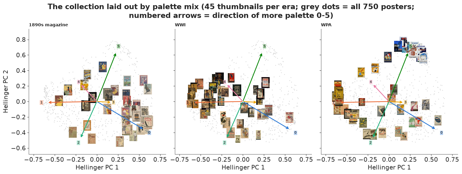
Two components keep 57% of the variation, enough to see the eras separate: 1890s posters lie towards palettes 0 and 3 (paper and grey ink), WWI posters towards palettes 1 and 4 (ochre and black), and the WPA reaches a region the other eras barely enter - up the palette 5 arrow, where the white-and-blue silkscreens are. The WPA also has a group among the WWI-like ochres: the era is not one style.
F. How did palettes change from the 1890s to the WPA? And when was this poster made?
Plain LDA gives every document the same prior mixture. To ask how palettes depend on something about a document - its era, its publisher, its campaign - the prior of $\theta_d$ must depend on covariates. Two classic designs do this. The structural topic model (Roberts et al. 2014, widely used in the social sciences) replaces the Dirichlet by a logistic normal whose mean depends on covariates; Dirichlet-multinomial regression (Mimno & McCallum 2008) keeps the Dirichlet and lets covariates set its parameters. We try the logistic normal first, because it is Gaussian underneath and NUTS likes that:
$$\boldsymbol\eta_d \sim \text{Normal}\big(\boldsymbol\mu_{\text{era}(d)},\; \tau^2 I\big),\qquad \boldsymbol\theta_d = \text{softmax}(\boldsymbol\eta_d),\qquad \mathbf n_d \sim \text{Multinomial}(200,\; \boldsymbol\theta_d^\top \Phi),$$
with the last palette's $\eta$ fixed at 0 (softmax does not change if a constant is added to every $\eta$, so one reference palette is needed). $\boldsymbol\mu_{\text{era}}$ is an era's typical palette mix on the log-odds scale and $\tau$ how much posters of one era differ.
The palettes $\Phi$ are held fixed at the posterior mean of the best restart. While preparing the notebook, fitting them jointly with this model took over 4 minutes with almost every transition at tree depth 9 or 10 - palettes and mixtures trade off against each other, $\Theta\Phi = (\Theta A)(A^{-1}\Phi)$ for many matrices $A$ that keep both on the simplex - while the palette posterior itself is very narrow (its largest sd was printed above).
Dating posters. We hide the era of a random 20% of posters and let the model infer it. A poster without a label gets the era mixture as its prior, $p(\boldsymbol\eta_d) = \sum_{e} \tfrac13\, \text{Normal}(\boldsymbol\eta_d \mid \boldsymbol\mu_e, \tau^2 I)$, so labelled and unlabelled posters are fitted together (a semi-supervised topic model), and each hidden poster's era probabilities come out of the posterior. The palettes were learned without looking at any era label, so nothing leaks.
hide = np.random.default_rng(4).random(len(X_col)) < 0.2
lab_i, unl_i = np.flatnonzero(~hide), np.flatnonzero(hide)
phi_fixed = np.clip(phi_col, 1e-6, None)
phi_fixed /= phi_fixed.sum(1, keepdims=True)
Km1 = K_COL - 1
theta_start = np.clip(theta_col, 1e-3, None)
theta_start /= theta_start.sum(1, keepdims=True)

# starting values from the Gibbs mixtures (log-odds against the reference palette)
eta0 = np.log(theta_start)
eta0 = eta0[:, :Km1] - eta0[:, [Km1]]
mu0 = np.array([eta0[lab_i][era_idx[lab_i] == e].mean(0) for e in range(3)])
coords_era = {"era": ERAS, "free_palette": [f"palette {k}" for k in range(Km1)],
              "palette": [f"palette {k}" for k in range(K_COL)], "labelled": lab_i, "hidden": unl_i}
with pm.Model(coords=coords_era) as ln_model:
    mu = pm.Normal("mu", 0, 3, dims=("era", "free_palette"))
    tau = pm.HalfNormal("tau", 3)
    eta_lab = pm.Normal("eta_lab", mu[era_idx[lab_i]], tau, dims=("labelled", "free_palette"))
    eta_hid = pm.Flat("eta_hid", dims=("hidden", "free_palette"))
    # era mixture prior for the hidden posters, with the era summed out
    comp = (-0.5 * ((eta_hid[:, None, :] - mu[None]) / tau) ** 2
            - pt.log(tau) - 0.5 * np.log(2 * np.pi)).sum(-1)                      # hidden x era
    pm.Potential("era_mixture", pt.logsumexp(comp + np.log(1 / 3), axis=1).sum())

    def softmax_ref(eta):
        return pm.math.softmax(pt.concatenate([eta, pt.zeros((eta.shape[0], 1))], axis=1), axis=1)

    pm.Multinomial("x_lab", n=N_TOK, p=softmax_ref(eta_lab) @ phi_fixed, observed=X_col[lab_i])
    pm.Multinomial("x_hid", n=N_TOK, p=softmax_ref(eta_hid) @ phi_fixed, observed=X_col[hide])
    pm.Deterministic("era_logp", comp, dims=("hidden", "era"))

t0 = time.perf_counter()
idata_ln = pm.sample(model=ln_model, random_seed=RANDOM_SEED, progressbar=False,
                     initvals={"mu": mu0, "tau": 2.0, "eta_lab": eta0[lab_i], "eta_hid": eta0[hide]},
                     var_names=["mu", "tau", "era_logp"])
print(f"sampled in {time.perf_counter() - t0:.0f} s; divergences: {int(idata_ln.sample_stats['diverging'].sum())}; "
      f"tree depth: {np.bincount(idata_ln.sample_stats['depth'].values.ravel())}")
print(az.summary(idata_ln, var_names=["tau"], round_to=3)[["mean", "sd", "r_hat", "ess_bulk"]])
print("max r_hat of mu:", round(float(az.rhat(idata_ln.posterior["mu"]).max()), 3))
sampled in 51 s; divergences: 0; tree depth: [   0    0    0    0    0    0    0 3322  678]
      mean     sd  r_hat  ess_bulk
tau  3.923  0.074  1.001  1214.489
max r_hat of mu: 1.002
The sampler is happy. ($\hat R$ and ESS are fine within the palette solution we conditioned on; the chains started from the Gibbs solution and did not have to find the palettes, so this says nothing about the other palette sets of part E.) Now the hidden posters. For each posterior draw, a hidden poster's era probabilities are its normalised mixture components; averaging over draws gives $P(\text{era} \mid \text{palette})$. We score them three ways: accuracy, the mean log score (chance: $\log \tfrac13 = -1.10$), and calibration - when the model says 80%, is it right 80% of the time?
truth = era_idx[hide]


def era_probs(idata):
    lp = idata.posterior["era_logp"].values                            # chain, draw, hidden, era
    p = np.exp(lp - lp.max(-1, keepdims=True))
    return (p / p.sum(-1, keepdims=True)).mean((0, 1))


def dating_report(p, name):
    pred, top = p.argmax(1), p.max(1)
    print(f"{name}: accuracy {np.mean(pred == truth):.2f} (chance 0.33), mean log score "
          f"{np.mean(np.log(p[np.arange(len(truth)), truth])):.3f} (chance {np.log(1 / 3):.3f})")
    for lo_, hi_ in [(0.33, 0.6), (0.6, 0.8), (0.8, 1.01)]:
        sel = (top >= lo_) & (top < hi_)
        if sel.any():
            print(f"   stated top probability {lo_:.2f}-{min(hi_, 1):.2f}: {sel.sum():3d} posters, "
                  f"mean stated {top[sel].mean():.2f}, actually correct {np.mean(pred[sel] == truth[sel]):.2f}")


p_ln = era_probs(idata_ln)
dating_report(p_ln, "logistic normal")
logistic normal: accuracy 0.55 (chance 0.33), mean log score -1.128 (chance -1.099)
   stated top probability 0.33-0.60:  44 posters, mean stated 0.50, actually correct 0.45
   stated top probability 0.60-0.80:  50 posters, mean stated 0.71, actually correct 0.58
   stated top probability 0.80-1.00:  48 posters, mean stated 0.89, actually correct 0.60
Better than chance at picking the era (0.55 against 0.33) - and yet the log score is worse than guessing (-1.13 against -1.10). The model is overconfident: when it says about 0.89, it is right 60% of the time. A classifier that is right more often than chance but loses to "I don't know" on log score is making some confident mistakes that cost a lot.
The cause is the logistic normal's shape. A palette that is (almost) absent from a poster has a very negative log-odds $\eta_{dk}$, and the only thing holding it is the Gaussian prior, which is quadratic in $\eta$. The large $\tau$ (about 3.9) is the model stretching to cover these far tails, and the eras' Gaussians disagree steeply out there: small differences in how absent a palette is become big differences in era probability.
The Dirichlet does not have this problem. Its log-density is linear in the log-shares, $\sum_k (\alpha_k - 1)\log\theta_k$, so a palette that is absent from a poster costs a bounded, gentle amount, and a small $\alpha_k$ says "absent is normal". So: Dirichlet-multinomial regression, with one Dirichlet per era,
$$\boldsymbol\theta_d \sim \text{Dirichlet}(\boldsymbol\alpha_{\text{era}(d)}), \qquad \log\alpha_{ek} \sim \text{Normal}(\log 0.5,\; 1.5).$$
Its mean $\boldsymbol\alpha_e / \sum_k \alpha_{ek}$ is the era's average palette mix, and its total $\sum_k \alpha_{ek}$ how alike the era's posters are (small = each poster uses few palettes).
How to sample it matters. pm.Dirichlet works (while preparing: 295 s, almost every transition
at the maximum tree depth, and similar answers). Faster is the textbook construction: if
$g_k \sim \text{Gamma}(\alpha_k, 1)$ independently, then $\mathbf g / \sum_k g_k$ is
$\text{Dirichlet}(\boldsymbol\alpha)$. Sample $u_k = \log g_k$, whose density is
$\exp(\alpha_k u_k - e^{u_k}) / \Gamma(\alpha_k)$, and set $\boldsymbol\theta = \text{softmax}(\mathbf u)$.
The scale $\sum_k g_k$ is an extra direction the data never see, but its prior keeps it in
place. For a hidden poster the prior of $\mathbf u$ is the equal-weight mixture over eras of
these densities, which is exact.
with pm.Model(coords=coords_era) as dmr_model:
    log_alpha = pm.Normal("log_alpha", np.log(0.5), 1.5, dims=("era", "palette"))
    alpha = pt.exp(log_alpha)
    u_lab = pm.Flat("u_lab", dims=("labelled", "palette"))
    a_lab = alpha[era_idx[lab_i]]
    pm.Potential("gamma_lab", (a_lab * u_lab - pt.exp(u_lab) - pt.gammaln(a_lab)).sum())
    u_hid = pm.Flat("u_hid", dims=("hidden", "palette"))
    comp = (alpha[None] * u_hid[:, None, :] - pt.exp(u_hid)[:, None, :] - pt.gammaln(alpha)[None]).sum(-1)
    pm.Potential("era_mixture", pt.logsumexp(comp + np.log(1 / 3), axis=1).sum())
    pm.Multinomial("x_lab", n=N_TOK, p=pm.math.softmax(u_lab, axis=1) @ phi_fixed, observed=X_col[lab_i])
    pm.Multinomial("x_hid", n=N_TOK, p=pm.math.softmax(u_hid, axis=1) @ phi_fixed, observed=X_col[hide])
    pm.Deterministic("era_logp", comp, dims=("hidden", "era"))

t0 = time.perf_counter()
idata_dmr = pm.sample(model=dmr_model, random_seed=RANDOM_SEED, progressbar=False,
                      initvals={"log_alpha": np.full((3, K_COL), np.log(0.5)),
                                "u_lab": np.log(theta_start[lab_i]), "u_hid": np.log(theta_start[hide])},
                      var_names=["log_alpha", "era_logp"])
print(f"sampled in {time.perf_counter() - t0:.0f} s; divergences: {int(idata_dmr.sample_stats['diverging'].sum())}; "
      f"tree depth: {np.bincount(idata_dmr.sample_stats['depth'].values.ravel())}")
print("max r_hat of log alpha:", round(float(az.rhat(idata_dmr.posterior["log_alpha"]).max()), 3),
      "| min bulk ESS:", int(az.ess(idata_dmr.posterior["log_alpha"]).min()))
p_dmr = era_probs(idata_dmr)
dating_report(p_ln, "logistic normal")
dating_report(p_dmr, "Dirichlet     ")
sampled in 151 s; divergences: 0; tree depth: [   0    0    0    0    0    0    0    0 4000]
max r_hat of log alpha: 1.015 | min bulk ESS: 569
logistic normal: accuracy 0.55 (chance 0.33), mean log score -1.128 (chance -1.099)
   stated top probability 0.33-0.60:  44 posters, mean stated 0.50, actually correct 0.45
   stated top probability 0.60-0.80:  50 posters, mean stated 0.71, actually correct 0.58
   stated top probability 0.80-1.00:  48 posters, mean stated 0.89, actually correct 0.60
Dirichlet     : accuracy 0.48 (chance 0.33), mean log score -1.022 (chance -1.099)
   stated top probability 0.33-0.60:  67 posters, mean stated 0.52, actually correct 0.46
   stated top probability 0.60-0.80:  50 posters, mean stated 0.71, actually correct 0.40
   stated top probability 0.80-1.00:  25 posters, mean stated 0.85, actually correct 0.68
fig, ax = plt.subplots(figsize=(5.5, 4.2))
bins = np.array([1 / 3, 0.5, 0.65, 0.8, 1.0001])
for p, name, col in [(p_ln, "logistic normal", "C3"), (p_dmr, "Dirichlet", "C0")]:
    top, correct = p.max(1), p.argmax(1) == truth
    b = np.digitize(top, bins) - 1
    xs = [top[b == j].mean() for j in range(len(bins) - 1) if np.any(b == j)]
    ys = [correct[b == j].mean() for j in range(len(bins) - 1) if np.any(b == j)]
    ns = [np.sum(b == j) for j in range(len(bins) - 1) if np.any(b == j)]
    ax.plot(xs, ys, "o-", color=col, label=name)
    for x_, y_, n_ in zip(xs, ys, ns):
        ax.annotate(str(n_), (x_, y_), textcoords="offset points", xytext=(4, -10), fontsize=7, color=col)
ax.plot([1 / 3, 1], [1 / 3, 1], color="k", lw=0.8, ls="--")
ax.set(xlabel="stated probability of the most likely era", ylabel="share actually correct",
       title="Calibration of poster dating (142 hidden posters;\nnumbers = posters per bin)")
ax.legend(fontsize=8);
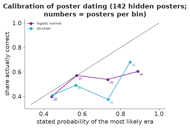
The Dirichlet model samples cleanly (zero divergences, $\hat R$ about 1.01) in about two and a half minutes, at tree depth 8. For dating it is the better probabilistic model: its log score, -1.02, beats both guessing (-1.10) and the logistic normal (-1.13), and its most confident datings (about 25 posters stated at about 0.85) are right about 70% of the time. It is not simply better: its accuracy is lower (0.48 against 0.55), and posters it gives 0.6-0.8 are right only about 40% of the time. With 142 posters these bins are noisy, but the picture is clear enough: colour alone dates a poster only roughly, and the prior shape decides how honest the model is about that. Both models are overconfident - part G suggests one reason.
What did each era look like? From the Dirichlet model, an era's average palette mix is $\boldsymbol\alpha_e / \sum_k \alpha_{ek}$, for every posterior draw.
alpha_draws = np.exp(az.extract(idata_dmr, var_names=["log_alpha"]).transpose("sample", "era", "palette").values)
share = alpha_draws / alpha_draws.sum(-1, keepdims=True)                 # draw, era, palette
conc = alpha_draws.sum(-1)
print("Dirichlet total (small = each poster uses few palettes), posterior mean:",
      dict(zip(ERAS, conc.mean(0).round(2))))

fig, axes = plt.subplots(1, 2, figsize=(12, 5.2), width_ratios=[1.3, 1])
for e in range(3):
    lo, hi = np.quantile(share[:, e], [0.05, 0.95], axis=0)
    mid = share[:, e].mean(0)
    axes[0].errorbar(np.arange(K_COL) + (e - 1) * 0.22, mid, yerr=[mid - lo, hi - mid], fmt="o",
                     color=f"C{e}", label=ERAS[e])
axes[0].set_xticks(range(K_COL), [str(k) for k in range(K_COL)])
axes[0].set(ylabel="average share of a poster (90% interval)", title="Palette mix by era (palettes 0-5, strips below)")
axes[0].legend(fontsize=8)
for k in range(K_COL):                                              # palette squares under the axis
    ins = axes[0].inset_axes([k / K_COL + 0.02, -0.34, 1 / K_COL - 0.04, 0.2], transform=axes[0].transAxes)
    palette_squares(ins, phi_col[k], labels=False)
mean_share = share.mean(0)                                          # era x palette
for e in range(3):                                                  # 100% bars, segments filled with the palette
    left = 0.0
    for k in range(K_COL):
        w_k = mean_share[e, k]
        o = display_order
        widths = phi_col[k][o] * (w_k - 0.004)                          # 0.004 leaves a white gap
        axes[1].barh(e, widths, left=left + np.r_[0, np.cumsum(widths)[:-1]], height=0.62,
                     color=swatch[o], lw=0)
        axes[1].plot([left + w_k / 2], [e + 0.43], "s", ms=6, color=PALETTE_IDS[k])
        if w_k > 0.06:
            axes[1].text(left + w_k / 2, e + 0.52, f"{k}: {w_k:.0%}", ha="center", va="top", fontsize=7, color=INK)
        left += w_k
axes[1].set(xlim=(0, 1), ylim=(2.75, -0.5), xlabel="share of an average poster")
axes[1].set_yticks(range(3), ERAS)
axes[1].grid(False)
axes[1].set_title("Era composition: each segment is one palette, drawn in its own colours\n"
                  "(square = palette identity; label = palette: share)", fontsize=9)
Dirichlet total (small = each poster uses few palettes), posterior mean: {'1890s magazine': np.float64(1.49), 'WWI': np.float64(1.81), 'WPA': np.float64(1.08)}Text(0.5, 1.0, 'Era composition: each segment is one palette, drawn in its own colours\n(square = palette identity; label = palette: share)')
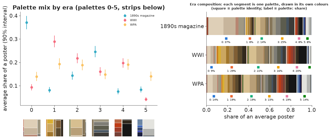
fig, axes = plt.subplots(1, 3, figsize=(12, 4.6))
for e, ax in enumerate(axes):
    palette_squares(ax, mean_share[e] @ phi_col, min_label=0.04)
    ax.set_title(ERAS[e], fontsize=11)
fig.suptitle("The colours of an average poster in each era, as areas (colour families in hue order, then beige, brown, grey)");
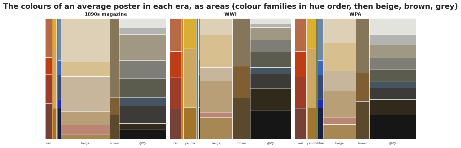
pairs = [(0, 1), (1, 2), (0, 2)]
diff = pd.DataFrame({f"{ERAS[b]} - {ERAS[a]}": (share[:, b] - share[:, a]).mean(0) for a, b in pairs},
                    index=[f"palette {k}" for k in range(K_COL)])
prob = pd.DataFrame({f"P({ERAS[b]} > {ERAS[a]})": (share[:, b] > share[:, a]).mean(0) for a, b in pairs},
                    index=diff.index)
print(pd.concat([diff.round(3), prob.round(3)], axis=1))
           WWI - 1890s magazine  WPA - WWI  WPA - 1890s magazine  P(WWI > 1890s magazine)  P(WPA > WWI)  P(WPA > 1890s magazine)
palette 0                -0.277      0.046                -0.231                      0.0         1.000                    0.000
palette 1                 0.208     -0.097                 0.112                      1.0         0.000                    1.000
palette 2                 0.074     -0.028                 0.046                      1.0         0.072                    0.995
palette 3                -0.085     -0.012                -0.097                      0.0         0.241                    0.000
palette 4                 0.121     -0.007                 0.114                      1.0         0.360                    1.000
palette 5                -0.042      0.098                 0.057                      0.0         1.000                    1.000
The history of the three eras is readable in the palette shares (left: each palette's share with its interval; right: the same shares as one bar per era, each segment painted with its palette, so the overall look of an era is visible at a glance; and the three squares, the colours of an average poster of each era):
- 1890s magazine posters are paper and ink: palette 0 (cream paper) makes up about 37% of an average poster and the greys of palette 3 another 25%. Their Dirichlet total (about 1.5) says a typical poster uses one or two palettes.
- WWI posters swap the paper for full-colour lithography on dark grounds: the ochre-brown palette 1 (about 29%, more than three times the 1890s share) and black-red palette 4 (about 20%) take over, and white-blue palette 5 all but disappears.
- WPA posters keep black-red palette 4 at the WWI level, use less ochre-brown (palette 1 falls from about 29% to 19%), and bring back light grounds: white-blue palette 5 rises from about 4% to 14% (P > 0.99), and cream paper rises a little (silkscreens on light stock).
Every pairwise change marked with P = 0 or 1 in the table is certain given this palette solution; the restart table of part E is the reminder that palettes 1 and 3 are not the only way to cut the dark colours.
top_dmr = p_dmr.max(1)
show = np.r_[np.argsort(-top_dmr)[:4], np.argsort(top_dmr)[:4]]
fig, axes = plt.subplots(2, 8, figsize=(13, 4), height_ratios=[2.2, 1])
for c, j in enumerate(show):
    i = unl_i[j]
    r0, r1, c0, c1 = boxes[i]
    axes[0, c].imshow(thumbs[i][r0:r1, c0:c1])
    axes[0, c].axis("off")
    axes[0, c].set_title(f"{poster_year[i]}: {ERAS[era_idx[i]]}", fontsize=7)
    axes[1, c].bar(range(3), p_dmr[j], color=["C0", "C1", "C2"])
    axes[1, c].set(ylim=(0, 1), xticks=range(3), yticks=[0, 0.5, 1] if c == 0 else [])
    axes[1, c].set_xticklabels(["1890s", "WWI", "WPA"], fontsize=7)
fig.suptitle("Hidden posters, Dirichlet model: the four most confident datings (left) and the four least (right)");
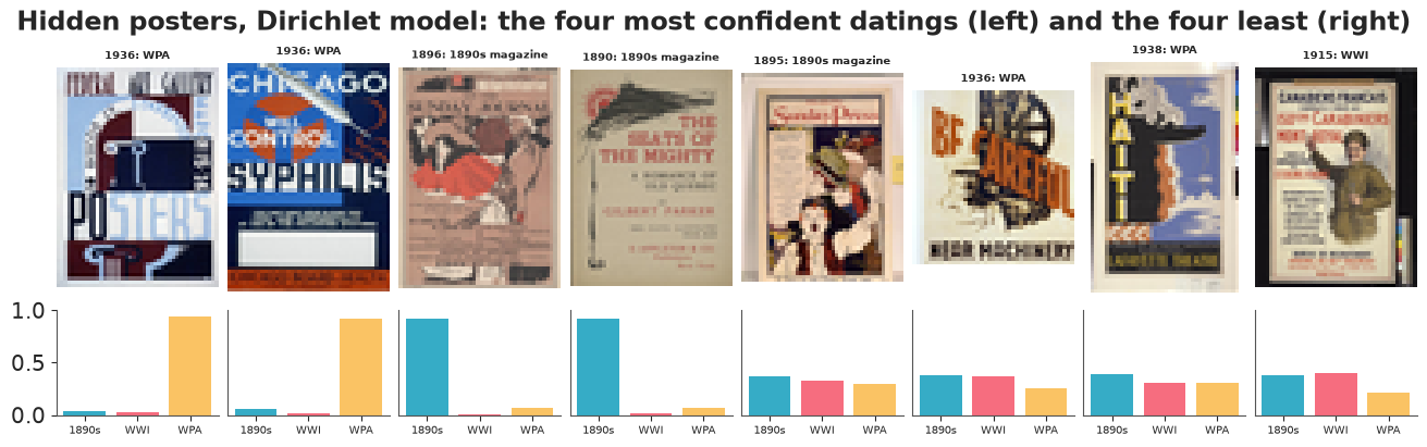
The easy cases sit at the extremes of the palette space: white-and-blue WPA silkscreens and cream-paper 1890s posters. The hard ones borrow another era's colours - a colourful 1890s lithograph, WPA and WWI posters on light cream paper. Nothing in a palette alone can date those; subject matter, typography and text would.
G. How much is a picture worth?
Every result above used 200 tokens per poster. The multinomial treats them as independent draws, so its certainty grows like $\sqrt N$: with all of a crop's ~2,600 pixels, every interval above would shrink by a factor of about 3.6. Is that real information or pseudo- replication?
A direct check: split each cropped poster into its top and bottom halves and compare their colour counts. If pixels were independent draws from one colour distribution, the halves would differ only by multinomial noise, and the chi-square statistic for "same distribution" would be about its degrees of freedom. The ratio statistic / df is an overdispersion factor: the number of pixels that behave like one independent token. Dividing a poster's pixel count by it gives an effective number of tokens.
(Posters are designed, and a top half - a title - can legitimately differ from a bottom half - a picture. That makes the check conservative: it can only overstate how much pixels disagree, and so understate the effective number of tokens a little, never overstate it.)
def overdispersion(words, V):
    half = len(words) // 2
    a, b = np.bincount(words[:half], minlength=V), np.bincount(words[half:2 * half], minlength=V)
    keep_w = (a + b) > 0
    a, b = a[keep_w], b[keep_w]
    expected = (a + b) / 2
    chi2 = np.sum((a - expected) ** 2 / expected) * 2
    return chi2 / max(keep_w.sum() - 1, 1)


# words were computed row by row (row-major), so the first half of the pixels is the top half
disp = np.array([overdispersion(w, V_COL) for w in poster_words])
n_pix = np.array([len(w) for w in poster_words])
n_eff = n_pix / np.maximum(disp, 1)
print(f"pixels per cropped poster: median {np.median(n_pix):.0f}")
print(f"overdispersion (chi2 / df, 1 = independent pixels): median {np.median(disp):.0f}, "
      f"quartiles {np.percentile(disp, 25):.0f}-{np.percentile(disp, 75):.0f}")
print(f"effective independent tokens per poster: median {np.median(n_eff):.0f}, "
      f"quartiles {np.percentile(n_eff, 25):.0f}-{np.percentile(n_eff, 75):.0f}")

# a within-half check with no design difference: odd vs even columns of the same rows
disp_cols = []
for t, (r0, r1, c0, c1), w in zip(thumbs, boxes, poster_words):
    grid = w.reshape(r1 - r0, c1 - c0)
    disp_cols.append(overdispersion(np.r_[grid[:, ::2].ravel(), grid[:, 1::2].ravel()[: grid[:, ::2].size]], V_COL))
print(f"odd vs even columns (neighbouring pixels): median chi2 / df {np.median(disp_cols):.1f}")

fig, ax = plt.subplots(figsize=(8, 3.2))
ax.hist(np.clip(n_eff, 1, 3000), bins=np.geomspace(1, 3000, 40), color="C0", alpha=0.8)
ax.axvline(N_TOK, color="k", lw=1)
ax.text(N_TOK * 1.1, ax.get_ylim()[1] * 0.9, f"{N_TOK} tokens used", fontsize=8)
ax.axvline(np.median(n_pix), color="C3", lw=1, ls="--")
ax.text(np.median(n_pix) * 1.05, ax.get_ylim()[1] * 0.75, "all pixels", fontsize=8, color="C3")
ax.set(xscale="log", xlabel="effective independent tokens per poster (pixels / overdispersion)",
       ylabel="posters", title="How many independent colour draws is a poster worth?");
pixels per cropped poster: median 2640
overdispersion (chi2 / df, 1 = independent pixels): median 20, quartiles 12-33
effective independent tokens per poster: median 120, quartiles 72-196
odd vs even columns (neighbouring pixels): median chi2 / df 1.7
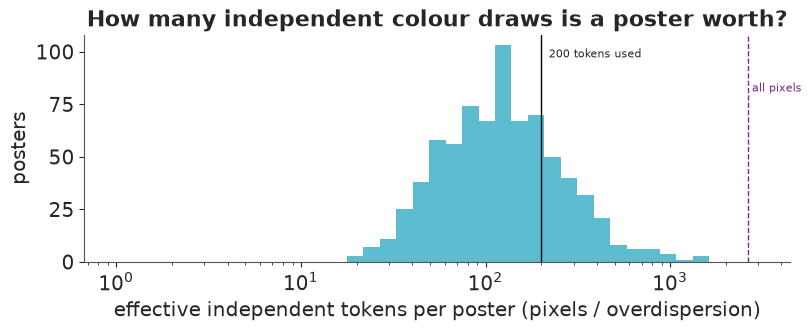
Top and bottom halves of the same poster disagree about 20 times more than independent pixels would (median chi-square / df; quartiles 12-33). Dividing each poster's ~2,600 pixels by that factor gives a median of about 120 effective independent colour draws per poster. Neighbouring columns, on the other hand, agree almost perfectly (chi-square / df 1.7): the pixels are near-copies of their neighbours, so adding them adds almost nothing.
So the 200 tokens we used overstate a typical poster's evidence by a factor of about 1.7 (so intervals about 1.3 times too narrow), and using every pixel would have overstated it about 20-fold (intervals about 4.7 times too narrow). This is one plausible contributor to the overconfident dating of part F (exercise 1 tests it). Two remedies:
- choose the number of tokens per document from a check like this one (here about 100-120), or
- keep all pixels and temper the likelihood by $N_\text{eff}/N$ (a "power likelihood"), which has the same effect on uncertainty.
The same question arises whenever a "document" is built from correlated measurements: repeated words within one text, sessions from one user, reads from one sequencing library.
H. Two more bags of features: web sessions and shopping baskets
The same model, and the same code, on the two business uses from the table at the top.
H1. Web analytics: browsing intents on a news site
The msnbc.com anonymous web data (Heckerman 1999, UCI) records every page request made to msnbc.com and the news pages of msn.com on 28 September 1999, at the level of 17 page categories (front page, news, sports, weather, ...). A session - one user's requests that day - is the document and the categories are its words, so a topic is a browsing intent: a set of sections that tend to be visited together. We use a 60,000-session random sample and keep sessions with 2 to 100 page views (a single view has no co-occurrence to learn from; a few sessions with thousands of views are robots). Order within a session is ignored by LDA, but we will use it to test prediction.
data.describe("msnbc_sessions")
web = data.load("msnbc_sessions")
CATEGORIES = np.array("frontpage news tech local opinion on-air misc weather msn-news health living business "
                      "msn-sports sports summary bbs travel".split())
sessions = [np.array(p.split(), int) - 1 for p in web["pages"]]
sessions = [s for s in sessions if 2 <= len(s) <= 100]
X_web = np.array([np.bincount(s, minlength=len(CATEGORIES)) for s in sessions])
print(f"{len(sessions):,} sessions with 2-100 views (of {len(web):,}); median {np.median(X_web.sum(1)):.0f} views")

K_WEB = 6
phi_web_d, theta_web_d, _ = lda_gibbs(X_web, K_WEB, alpha=0.1, beta=0.1, burn=500, draws=20, thin=10, seed=1)
phi_web, theta_web = phi_web_d.mean(0), theta_web_d.mean(0)
web_order = np.argsort(-theta_web.mean(0))
phi_web, theta_web = phi_web[web_order], theta_web[:, web_order]
intents = [" + ".join(CATEGORIES[np.argsort(-phi_web[k])[:2]]) for k in range(K_WEB)]

fig, ax = plt.subplots(figsize=(12, 3.8))
cat_order = np.argsort(-X_web.sum(0))
for k in range(K_WEB):
    ax.scatter(np.arange(len(CATEGORIES)), np.full(len(CATEGORIES), k), s=phi_web[k, cat_order] * 1400,
               color=TOPIC_COLOURS[k], alpha=0.85, edgecolor="white", lw=1)
    ax.text(len(CATEGORIES) - 0.3, k, f"{theta_web[:, k].mean():.0%} of views", va="center", fontsize=8, color=INK)
ax.set_xticks(range(len(CATEGORIES)), CATEGORIES[cat_order], rotation=40, ha="right", fontsize=8)
ax.set_yticks(range(K_WEB), [f"intent {k}: {intents[k]}" for k in range(K_WEB)], fontsize=8)
ax.set(xlim=(-0.7, len(CATEGORIES) + 1.3), ylim=(K_WEB - 0.5, -0.6),
       title="Browsing intents on msnbc.com (circle area = share of the intent's page views; "
             "categories ordered by overall traffic)")
ax.grid(False);
msnbc_sessions: One row per user session (all page requests of one user that day): session (line number in the original file, from 0), n_views, pages (space-separated page-category codes in request order: 1 frontpage, 2 news, 3 tech, 4 local, 5 opinion, 6 on-air, 7 misc, 8 weather, 9 msn-news, 10 health, 11 living, 12 business, 13 msn-sports, 14 sports, 15 summary, 16 bbs, 17 travel). Cached pages were not logged.
  source: Heckerman, D. (1999), msnbc.com anonymous web data, UCI Machine Learning Repository (CC BY 4.0): IIS logs of msnbc.com and the news parts of msn.com for 28 September 1999, 989,818 users. SUBSAMPLED by tools/build_e72_extras.py (seed 72): 60,000 random sessions - keep the cached file in data/.
  url:    https://archive.ics.uci.edu/static/public/133/msnbc+com+anonymous+web+data.zip
37,590 sessions with 2-100 views (of 60,000); median 4 views
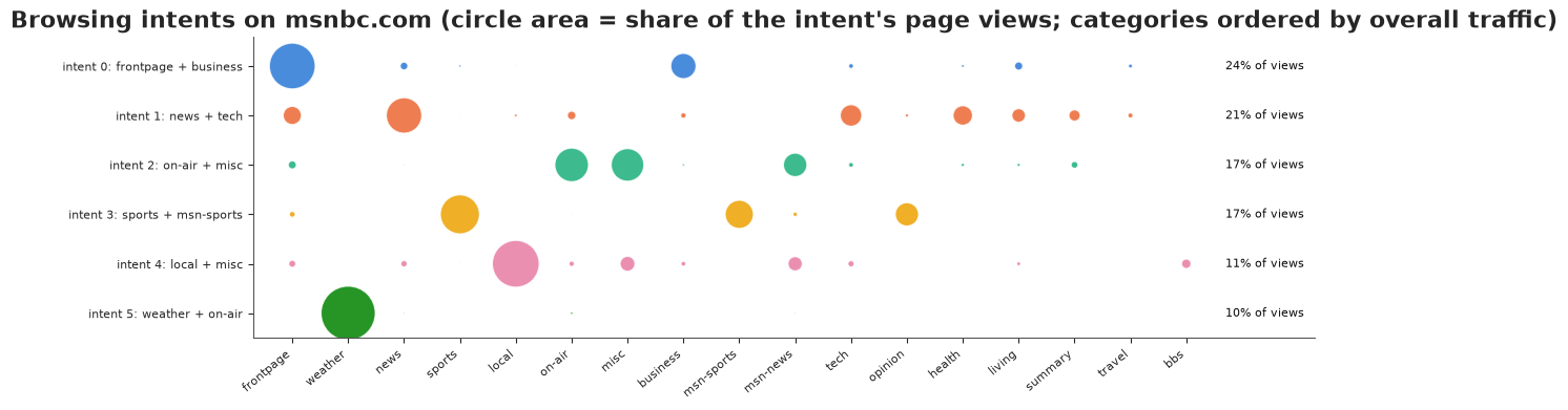
Six intents, each readable as a kind of visit. What do visits of each intent look like? A session "is" an intent when more than 80% of its mixture belongs to it.
lengths = X_web.sum(1)
dominant = theta_web.argmax(1)
pure = theta_web.max(1) > 0.8
print(f"{pure.mean():.0%} of sessions are more than 80% one intent")
print(pd.DataFrame({
    "share of sessions (dominant)": [np.mean(dominant == k) for k in range(K_WEB)],
    "of which > 80% pure": [np.mean(pure[dominant == k]) for k in range(K_WEB)],
    "median views": [np.median(lengths[dominant == k]) for k in range(K_WEB)],
    "mean views": [lengths[dominant == k].mean() for k in range(K_WEB)],
}, index=[f"intent {k}: {intents[k]}" for k in range(K_WEB)]).round(2))
47% of sessions are more than 80% one intent
                                share of sessions (dominant)  of which > 80% pure  median views  mean views
intent 0: frontpage + business                          0.26                 0.46           4.0        6.38
intent 1: news + tech                                   0.21                 0.42           4.0        6.40
intent 2: on-air + misc                                 0.17                 0.42           4.0        6.62
intent 3: sports + msn-sports                           0.17                 0.53           4.0        6.58
intent 4: local + misc                                  0.09                 0.36           4.0        7.69
intent 5: weather + on-air                              0.10                 0.66           6.0        7.39
Can intents predict where a visit goes next? A realistic test: hold out 20% of the sessions with at least four views, show the model the first half of each (in the order requested), and score its prediction of the categories of the second half. Two baselines: overall popularity, and "more of the same" - the session's own first-half counts smoothed towards popularity, $(n_{dw} + c\,p_w) / (n_d + c)$ with $c = 2$ (the best of a few values tried while preparing this notebook). We also score only the views of categories the visitor had not seen yet - where a model of intents should help most.
split_web = np.random.default_rng(12)
test_web = (split_web.random(len(X_web)) < 0.2) & (lengths >= 4)
X_web_train = X_web[~test_web]
test_rows = np.flatnonzero(test_web)
seen = np.array([np.bincount(sessions[i][: len(sessions[i]) // 2], minlength=len(CATEGORIES)) for i in test_rows])
rest = X_web[test_rows] - seen
new_mask = seen == 0
popular = (X_web_train.sum(0) + 0.5) / (X_web_train.sum() + 0.5 * len(CATEGORIES))


def predict_hidden(X_seen, phis, alpha=0.1, sweeps=50, seed=0):
    """Posterior predictive word probabilities for documents with the seen part only (topics fixed)."""
    g = np.random.default_rng(seed)
    d_i, w_i = np.nonzero(X_seen)
    n = X_seen[d_i, w_i]
    doc, word = np.repeat(d_i, n), np.repeat(w_i, n)
    K = phis.shape[1]
    prob = np.zeros(X_seen.shape)
    for s, phi_s in enumerate(phis):
        z = g.integers(K, size=doc.size)
        ndk = np.zeros((X_seen.shape[0], K), np.int64)
        np.add.at(ndk, (doc, z), 1)
        _foldin_sweeps(doc, word, z, ndk, phi_s, alpha, sweeps, seed + s)
        prob += (ndk + alpha) / (ndk.sum(1, keepdims=True) + K * alpha) @ phi_s
    return prob / len(phis)


def web_scores(p):
    all_views = np.sum(rest * np.log(p)) / rest.sum()
    q = p * new_mask
    q = q / q.sum(1, keepdims=True)
    new = rest * new_mask
    ok = new.sum(1) > 0
    return all_views, np.sum(new[ok] * np.log(np.clip(q[ok], 1e-300, None))) / new[ok].sum()


rows_web = {"popularity": np.tile(popular, (len(seen), 1)),
            "more of the same (c = 2)": (seen + 2 * popular) / (seen.sum(1, keepdims=True) + 2)}
for K in [6, 14]:
    phis_k, _, _ = lda_gibbs(X_web_train, K, alpha=0.1, beta=0.1, burn=300, draws=5, thin=20, seed=20 + K)
    rows_web[f"LDA, {K} intents"] = predict_hidden(seen, phis_k)
print(f"{len(test_rows):,} held-out sessions; {(rest * new_mask).sum() / rest.sum():.0%} of their second-half "
      "views are of categories not seen in the first half")
print(pd.DataFrame([web_scores(p) for p in rows_web.values()], index=list(rows_web),
                   columns=["log score per view", "log score, new categories only"]).round(3))
4,399 held-out sessions; 23% of their second-half views are of categories not seen in the first half
                          log score per view  log score, new categories only
popularity                            -2.551                          -2.571
more of the same (c = 2)              -1.644                          -2.571
LDA, 6 intents                        -1.858                          -2.767
LDA, 14 intents                       -1.656                          -2.622
Topics are an excellent description of this traffic and a poor predictor of it:
- Description. Six intents, each a recognisable kind of visit: the front page (with business), news (with tech, health, living and summaries), on-air and misc (TV-related pages), sports, local news, and weather - which is almost a topic of its own. Nearly half the sessions are more than 80% one intent, weather visits the most single-minded (two thirds pure) and slightly longer. For a site this is a segmentation of visits rather than of visitors, with mixed visits represented as mixtures instead of being forced into one cluster.
- Prediction. Knowing a visit's intents did not beat the simplest rule, "more of the same": people keep returning to the categories they have already opened, which the visit's own counts capture directly (-1.64 nats per view, against -1.66 for 14 intents and -1.86 for 6). For the pages a visitor had not yet opened - 23% of the second-half views - intents were worse than plain popularity (-2.62 and -2.77 against -2.57). With 17 broad categories there is little co-occurrence structure beyond "stay where you are". A sequence model (a Markov chain or a hidden Markov model over categories, see E24) is the natural next step for prediction.

H2. Retail: shopping missions of a gift wholesaler
The UCI Online Retail data (Chen, Sain & Guo 2012) are a year of orders (December 2010 to December 2011) from a UK online shop selling giftware, many of whose customers are small retailers. A customer is the document and the products they bought are its words, so a topic is a shopping mission - a set of products bought by the same kinds of customer. We keep products bought by at least 30 customers and customers who bought at least 10 of them, and record each product once per customer (bought or not): repeat orders of one product would otherwise dominate a wholesaler's "document".
data.describe("online_retail")
retail = data.load("online_retail")
product_names = data.load("online_retail_products").set_index("stock_code")["description"]
n_cust = retail.groupby("stock_code")["customer_id"].nunique()
retail = retail[retail["stock_code"].isin(n_cust.index[n_cust >= 30])]
n_prod = retail.groupby("customer_id")["stock_code"].nunique()
retail = retail[retail["customer_id"].isin(n_prod.index[n_prod >= 10])]
cust_i, customers = pd.factorize(retail["customer_id"])
prod_i, products = pd.factorize(retail["stock_code"])
X_ret = np.zeros((len(customers), len(products)), np.int64)
X_ret[cust_i, prod_i] = 1
names = product_names.loc[products].str.strip().str.lower().to_numpy()
cust_country = retail.groupby("customer_id")["country"].first().loc[customers].to_numpy()
print(f"{len(customers):,} customers x {len(products):,} products; median {np.median(X_ret.sum(1)):.0f} "
      f"products per customer")

K_RET = 10
t0 = time.perf_counter()
phi_ret_d, theta_ret_d, _ = lda_gibbs(X_ret, K_RET, alpha=0.1, beta=0.05, burn=500, draws=20, thin=10, seed=3)
print(f"fitted in {time.perf_counter() - t0:.0f} s")
phi_ret, theta_ret = phi_ret_d.mean(0), theta_ret_d.mean(0)
ret_order = np.argsort(-theta_ret.mean(0))
phi_ret, theta_ret = phi_ret[ret_order], theta_ret[:, ret_order]
p_prod = X_ret.sum(0) / X_ret.sum()
rel_ret = 0.6 * np.log(phi_ret) + 0.4 * np.log(phi_ret / p_prod)
online_retail: A UK online retailer of giftware (many customers are wholesalers), orders 1 Dec 2010 - 9 Dec 2011, one row per (customer, product): customer_id, country (the customer's most common), stock_code, n_invoices (orders containing the product), quantity (units). 4,335 customers, 3,659 products, 266,226 rows; cancellations, returns, rows without a customer and non-product codes (postage, fees, adjustments) removed. Product names: online_retail_products.
  source: Chen, D. (2015), Online Retail, UCI Machine Learning Repository (CC BY 4.0); Chen, Sain & Guo (2012), Journal of Database Marketing & Customer Strategy Management 19:197-208. AGGREGATED by tools/build_e72_extras.py from the 541,909 transaction lines of the spreadsheet at the URL - keep the cached file in data/.
  url:    https://archive.ics.uci.edu/static/public/352/online+retail.zip
3,661 customers x 2,087 products; median 43 products per customer
fitted in 5 s
fig, axes = plt.subplots(2, 5, figsize=(16, 7.5))
customers_in = (theta_ret * X_ret.sum(1)[:, None]).sum(0)
for k, ax in enumerate(axes.ravel()):
    top = np.argsort(-rel_ret[k])[:8][::-1]
    ax.barh(range(8), X_ret.sum(0)[top], color=GREY_BAR, height=0.72)
    ax.barh(range(8), phi_ret[k, top] * customers_in[k], color="#2a78d6", height=0.72)
    ax.set_yticks(range(8), [n[:26] for n in names[top]], fontsize=7)
    ax.set_title(f"mission {k} ({theta_ret[:, k].mean():.0%} of purchases)", fontsize=9, loc="left")
    ax.tick_params(axis="x", labelsize=7)
    ax.grid(axis="y", visible=False)
fig.supxlabel("customers buying the product: all (grey) and estimated within the mission (blue)", fontsize=9)
fig.suptitle("Ten shopping missions: the 8 most relevant products of each (relevance, lambda = 0.6)");
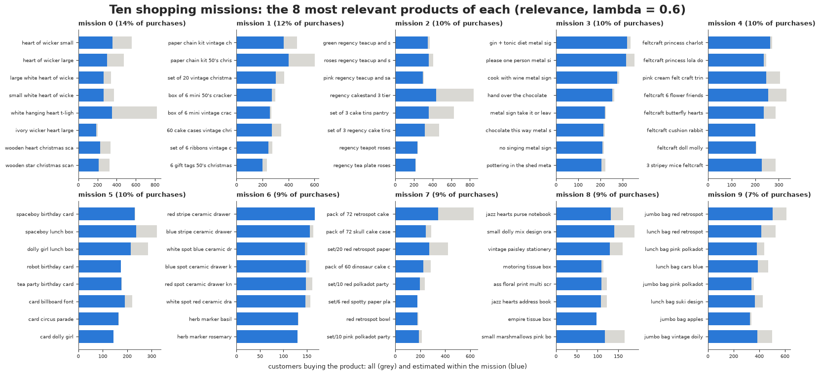
Who shops which mission? The shop's customers are mostly British, with a sizeable group of European businesses (Germany, France, the Benelux, Scandinavia, Iberia, ...). Averaging the mixtures by market, with a bootstrap over customers for the uncertainty, shows whether the European customers buy a different mix - the kind of question a merchandiser would ask before printing a catalogue for a market.
market = np.where(cust_country == "United Kingdom", "UK", "rest of the world")
market = np.where(np.isin(cust_country, ["Germany", "France", "EIRE", "Belgium", "Netherlands", "Switzerland",
                                          "Spain", "Portugal", "Italy", "Norway", "Finland", "Sweden",
                                          "Denmark", "Austria", "Poland", "Cyprus", "Channel Islands",
                                          "Greece", "Iceland", "Malta", "Lithuania", "Czech Republic"]),
                  "Europe (not UK)", market)
MARKETS = ["UK", "Europe (not UK)", "rest of the world"]
g_boot = np.random.default_rng(13)
fig, ax = plt.subplots(figsize=(10, 4.2))
for j, mk in enumerate(MARKETS):
    rows_m = np.flatnonzero(market == mk)
    boots = np.array([theta_ret[g_boot.choice(rows_m, len(rows_m))].mean(0) for _ in range(400)])
    lo, hi = np.quantile(boots, [0.05, 0.95], axis=0)
    mid = theta_ret[rows_m].mean(0)
    ax.errorbar(np.arange(K_RET) + (j - 1) * 0.22, mid, yerr=[mid - lo, hi - mid], fmt="o",
                color=["#2a78d6", "#eb6834", "#1baf7a"][j], label=f"{mk} ({len(rows_m)} customers)")
labels_ret = [names[np.argsort(-rel_ret[k])[0]][:18] for k in range(K_RET)]
ax.set_xticks(range(K_RET), [f"{k}: {labels_ret[k]}" for k in range(K_RET)], rotation=35, ha="right", fontsize=8)
ax.set(ylabel="average share of a customer's purchases\n(90% bootstrap interval)",
       title="Shopping missions by market")
ax.legend(fontsize=8);
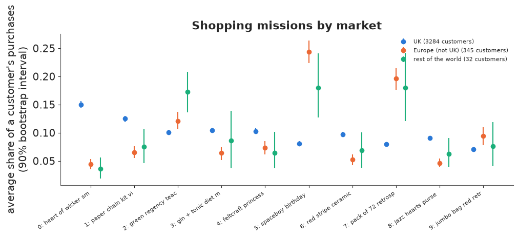
Recommending products. For a random 20% of customers we hide half of their products, infer each customer's mission mix from the other half, and recommend the ten most probable products they have not bought. The score is the hit rate: the share of the ten (or of all their hidden products, if fewer) that they did in fact buy. Baselines: the ten best-sellers, and the workhorse of recommender systems, item-to-item similarity (products scored by their cosine similarity, across customers, to what the customer already bought).
split_ret = np.random.default_rng(14)
test_ret = split_ret.random(len(X_ret)) < 0.2
X_ret_train, X_ret_test = X_ret[~test_ret], X_ret[test_ret]
shown = np.zeros_like(X_ret_test)
for d in range(len(X_ret_test)):
    bought = np.flatnonzero(X_ret_test[d])
    split_ret.shuffle(bought)
    shown[d, bought[: len(bought) // 2]] = 1
hidden = X_ret_test - shown


def hit_rate(score):
    score = np.where(shown > 0, -np.inf, score)
    top10 = np.argsort(-score, 1)[:, :10]
    return np.mean(np.take_along_axis(hidden, top10, 1).sum(1) / np.minimum(hidden.sum(1), 10))


col_norm = np.linalg.norm(X_ret_train, axis=0).clip(1e-9)
item_sim = (X_ret_train / col_norm).T @ (X_ret_train / col_norm)
np.fill_diagonal(item_sim, 0)
best_sellers = X_ret_train.sum(0).astype(float)
recs = {"best-sellers": np.tile(best_sellers, (len(shown), 1)),
        "item-to-item similarity": shown @ item_sim + 1e-9 * best_sellers}
t0 = time.perf_counter()
for K in [10, 40, 80]:
    phis_k, _, _ = lda_gibbs(X_ret_train, K, alpha=0.1, beta=0.05, burn=300, draws=5, thin=20, seed=30 + K)
    recs[f"LDA, {K} missions"] = predict_hidden(shown, phis_k)
print(f"LDA fits and predictions: {time.perf_counter() - t0:.0f} s; {len(shown)} held-out customers")
print(pd.Series({name: hit_rate(s) for name, s in recs.items()}, name="hit rate of the top 10").round(3))
LDA fits and predictions: 15 s; 750 held-out customers
best-sellers               0.109
item-to-item similarity    0.273
LDA, 10 missions           0.188
LDA, 40 missions           0.247
LDA, 80 missions           0.285
Name: hit rate of the top 10, dtype: float64
Here topics earn their keep in both ways:
- Description. The ten missions are the shop's product lines as customers actually combine them: wicker and wooden hearts (home decoration), vintage Christmas (paper chains, crackers), Regency tea sets and cake tins, humorous metal signs, feltcraft toys, children's party goods (birthday cards, lunch boxes), ceramic drawer knobs and herb markers, "retrospot" baking and party tableware, gift stationery, and bags. The market comparison is actionable: European customers put about three times the UK share of their purchases into children's party goods (about 0.24 against 0.08) and "retrospot" baking (0.20 against 0.08), and much less into the hearts, Christmas decorations, metal signs and drawer knobs. The 32 customers outside Europe are too few for firm conclusions (see their intervals).
- Prediction. Mission mixtures lift the hit rate of ten recommendations from 0.11 (best-sellers) to 0.19 with 10 missions, 0.25 with 40 and 0.29 with 80 - level with item-to-item similarity (0.27). Once more the number of topics depends on the purpose: ten missions to describe the business, eighty to recommend. LDA's advantages over item-to-item similarity are not accuracy but a posterior for every customer (with few purchases a customer's mixture is broad, which a recommender can use to hedge; item-to-item similarity has no notion of uncertainty) and missions a merchandiser can read.
Summary
- LDA is a model of any count table. Documents x features, each document a mixture of a few feature distributions: words in stories, colours in posters - and baskets, genomes, microbiomes and sessions in the same way.
- PyMC can fit it once the token topics are summed out, but label switching makes raw $\hat R$ meaningless (1.75 with zero divergences on simulated data; 1.008 after aligning chains with the Hungarian algorithm). On a sparse 650-word vocabulary NUTS struggled badly; a collapsed Gibbs sampler in Numba fits 4,468 documents in seconds.
- Stability is part of the answer. Some headline topics came back in every chain, others did not, while fake data from LDA itself were recovered almost exactly: instability is the mark of a model that fits real text only approximately. Report topics with their stability.
- Choose $K$ for the purpose. Held-out word prediction kept improving up to 80 topics (it rewards memorising stories); predicting click-through stopped improving at about 4.
- Uncertain regressors: plug in the posterior mean. Pooling regressions over posterior draws of the topic mixtures shrank every click-through effect by about a quarter, in a simulation with known effects as on the real data; the posterior-mean plug-in was unbiased. Multiple imputation needs an imputation model that sees the outcome.
- Pictures become documents with a CIELab colour vocabulary, once the scanner's contribution (backing and colour strips) is removed. Six palettes separate paper, ink, lithography and silkscreen without any labels.
- Covariates on the mixtures describe how palettes changed across eras and let the model date unlabelled posters. The prior's shape matters: a logistic normal was overconfident (log score worse than guessing); a Dirichlet, sampled as normalised log-Gammas, was better but still overconfident. Colour alone dates posters only roughly.
- Show topics where they live. Relevance-ranked words, a stability-aware topic map, words highlighted inside documents and prevalence over time explain word topics far better than a top-10 list; palettes read best on a lightness-hue map, as pixel segmentations of real posters (with a check of how well the model reproduces each poster's colours - roughly, here), in an atlas of thumbnails, and as era bars painted in their own colours.
- Web sessions and baskets. Browsing intents describe a news site's visits well but predicted the rest of a visit no better than "more of the same". Shopping missions describe a retailer's customers (and how Europe differs from the UK) and, with enough of them, recommend as well as item-to-item similarity - again, few topics to describe, many to predict.
- Pixels are not independent tokens: a poster is worth about 120 independent colour draws, not 2,600. How many tokens a document contributes is a modelling decision with consequences for every interval.
Try it yourself
- Temper the posters. Refit the Dirichlet era model with 100 tokens per poster (or all pixels
with the log-likelihood multiplied by $N_\text{eff}/N$ per poster, via
pm.Potential). Does the calibration of the dating improve? Does the log score? - Supervised LDA. Put the click-through regression inside the text model so that clicks and words inform the mixtures together: add the Normal likelihood of part C to the Gibbs sampler's full conditional for each token's topic (Blei & McAuliffe 2007 derive it). Do topics change? Do the effects move away from the plug-in estimates?
- Another bag of features. Use the same code on a different count table, for example the
bci_treesspecies counts per plot used in E30 (plots as documents, species as words: the topics are plant communities). Which parts of this notebook's checks carry over? - Orders instead of customers. Rebuild the retail corpus with orders as documents (the
UCI spreadsheet has invoice numbers;
tools/build_e72_extras.pyaggregates them away). Are order-level missions the same as customer-level ones? Which recommends better for the next order?