The question
Which products compete with which? A brand manager asks it to know whose customers a price cut will win. A retailer asks it to decide which products can share a shelf and which can be dropped. A competition authority asks it before letting two firms merge: if the merged firm raises the price of one product, how many of the lost customers will it recapture through the other? The answer is called the market structure of a category, and it is usually drawn as a tree (submarkets within submarkets) or a map (products close together compete hard).
The classic question for a category like margarine is whether the market is organised by form (stick buyers compare sticks; tub buyers compare tubs) or by brand (a Parkay buyer compares Parkay sticks with Parkay tubs), or by something else. Urban, Johnson & Hauser (1984), Grover & Srinivasan (1987) and Kannan & Wright (1991) all tested such hierarchies. We will test them, see why the classic test is weak, and build a model from which the structure can be read off instead of assumed.
The data are the scanner panel that Allenby & Rossi (1991) used to study asymmetric switching between brands of different quality: 516 households in two US cities, their margarine purchases in time order, and the price of every product on every shopping trip.
The decision we end with is an antitrust screen: if two margarine brands merged, would the merged firm have an incentive to raise prices?
The plan
- The data: shares, prices and the switching matrix
- The pooled logit and why it cannot see market structure
- The classic test: nested logits for competing hierarchies
- A choice map: household heterogeneity with a factor structure
- How many dimensions, and is loyalty real?
- A posterior predictive check on simulated purchase histories
- Reading the market structure off the posterior
- A merger screen
import logging
import time
import warnings

import arviz as az
import matplotlib.pyplot as plt
import numpy as np
import pandas as pd
import pymc as pm
import pytensor
import pytensor.tensor as pt
import xarray as xr
from matplotlib.patches import Ellipse
from scipy import special
from scipy.cluster import hierarchy

from pymc_challenges import data

RANDOM_SEED = 84
rng = np.random.default_rng(RANDOM_SEED)
az.style.use("arviz-variat")
logging.getLogger("pymc").setLevel(logging.WARNING)  # many fits: no sampler banner each
warnings.filterwarnings("ignore", category=RuntimeWarning, module="arviz")
warnings.filterwarnings("ignore", message="All-NaN slice")  # NaN diagonals of lift matrices
BLUE, ORANGE, AQUA, GREY, PURPLE, RED = "#2a78d6", "#eb6834", "#1baf7a", "#8a8a86", "#8c5ac8", "#c8384e"
print(f"PyMC {pm.__version__}, ArviZ {az.__version__}, PyTensor {pytensor.__version__}")


def q(x, probs=(0.05, 0.5, 0.95), axis=None):
    """Posterior quantiles, rounded for printing."""
    return np.round(np.quantile(x, probs, axis=axis), 2)
PyMC 6.3.2, ArviZ 1.3.0, PyTensor 3.3.2
data.describe("margarine")
df = data.load("margarine")
demos = data.load("margarine_demos")
PRODUCTS = ["Pk_Stk", "BB_Stk", "Fl_Stk", "Hse_Stk", "Gen_Stk", "Imp_Stk",
            "SS_Tub", "Pk_Tub", "Fl_Tub", "Hse_Tub"]
NAMES = {"Pk": "Parkay", "BB": "Blue Bonnet", "Fl": "Fleischmann's", "Hse": "House brand",
         "Gen": "Generic", "Imp": "Imperial", "SS": "Shedd's Spread"}
J = len(PRODUCTS)
df["y"] = df["choice"].map({p: j for j, p in enumerate(PRODUCTS)})
df["hh"] = pd.factorize(df["hhid"])[0]
H = df["hh"].max() + 1
price = df[[f"price_{p}" for p in PRODUCTS]].to_numpy()
print(f"{len(df):,} purchases by {H} households; purchases per household: "
      f"median {df.groupby('hh').size().median():.0f}, range "
      f"{df.groupby('hh').size().min()}-{df.groupby('hh').size().max()}")
df.head()
margarine: 4,470 margarine purchases by 516 households, in time order within household (no dates): hhid, trip (1, 2, ... within household), choice (one of 10 products: Pk = Parkay, BB = Blue Bonnet, Fl = Fleischmann's, Hse = the store's house brand, Gen = generic, Imp = Imperial, SS = Shedd's Spread; _Stk = sticks, _Tub = tub), and price_<product>: the shelf price (US$ per pound) of every product on that shopping trip.
  source: Allenby & Rossi (1991), 'Quality perceptions and asymmetric switching between brands', Marketing Science 10:185-205: an A.C. Nielsen scanner panel, distributed as `margarine` in the R package bayesm (Rossi; GPL >= 2; the URL is its CRAN source tarball). CONVERTED from .rda by tools/build_e84_margarine.py - keep the cached file.
  url:    https://cran.r-project.org/src/contrib/Archive/bayesm/bayesm_3.1-6.tar.gz
4,470 purchases by 516 households; purchases per household: median 7, range 1-43
| hhid | trip | choice | price_Pk_Stk | price_BB_Stk | price_Fl_Stk | price_Hse_Stk | price_Gen_Stk | price_Imp_Stk | price_SS_Tub | price_Pk_Tub | price_Fl_Tub | price_Hse_Tub | y | hh | |
|---|---|---|---|---|---|---|---|---|---|---|---|---|---|---|---|
| 0 | 2100016 | 1 | Pk_Stk | 0.66 | 0.67 | 1.09 | 0.57 | 0.36 | 0.93 | 0.85 | 1.09 | 1.19 | 0.33 | 0 | 0 |
| 1 | 2100016 | 2 | Pk_Stk | 0.63 | 0.67 | 0.99 | 0.57 | 0.36 | 1.03 | 0.85 | 1.09 | 1.19 | 0.37 | 0 | 0 |
| 2 | 2100016 | 3 | Pk_Stk | 0.29 | 0.50 | 0.99 | 0.57 | 0.36 | 0.69 | 0.79 | 1.09 | 1.19 | 0.59 | 0 | 0 |
| 3 | 2100016 | 4 | Pk_Stk | 0.62 | 0.61 | 0.99 | 0.57 | 0.36 | 0.75 | 0.85 | 1.09 | 1.19 | 0.59 | 0 | 0 |
| 4 | 2100016 | 5 | Pk_Stk | 0.50 | 0.58 | 0.99 | 0.45 | 0.33 | 0.72 | 0.85 | 1.07 | 1.19 | 0.59 | 0 | 0 |
share = df["choice"].value_counts(normalize=True).reindex(PRODUCTS).to_numpy()
fig, (a1, a2) = plt.subplots(1, 2, figsize=(12, 4), width_ratios=[1, 1.3])
col = [BLUE if p.endswith("Stk") else ORANGE for p in PRODUCTS]
a1.barh(PRODUCTS[::-1], share[::-1], color=col[::-1])
for j, s in enumerate(share[::-1]):
    a1.text(s + 0.005, j, f"{s:.1%}", va="center", fontsize=8)
a1.set_xlabel("share of purchases")
a1.set_title("Purchase shares (blue: sticks, orange: tubs)")
a2.boxplot(price[:, ::-1], orientation="horizontal", tick_labels=PRODUCTS[::-1], showfliers=False,
           medianprops=dict(color="k"))
a2.set_xlabel("shelf price on the trip (US$ per lb)")
a2.set_title("Prices vary from trip to trip (promotions)")
;
''
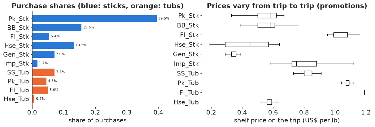
Parkay sticks take 40% of purchases; the house brand's tub less than 1%. Prices vary within each product mostly through temporary price cuts, and that variation identifies price sensitivity: the same household facing different relative prices on different trips. The spread differs a lot by product - Parkay and Blue Bonnet sticks are promoted often, Fleischmann's tub almost never - which will limit what we can learn about the tubs. The premium products (Fleischmann's, Imperial, the national-brand tubs) cost two to three times as much per pound as the house brand and generic.
1.2 · The switching matrix
The oldest tool of market structure analysis is the brand-switching matrix: count, for consecutive purchases of the same household, how often a purchase of product $k$ is followed by a purchase of product $j$. Two products that shoppers switch between often are, the argument goes, in the same submarket.
Raw counts mostly reflect size (everyone switches to Parkay because everyone buys Parkay), so we compare each off-diagonal count with what it would be if a switcher leaving $k$ picked the next product in proportion to overall shares, $s_j / (1 - s_k)$. The ratio is the switching lift: above 1, $k$ and $j$ exchange more buyers than their sizes predict.
df["prev"] = df.groupby("hh")["y"].shift()
pairs = df.dropna(subset="prev")
sw = pd.crosstab(pairs["prev"].astype(int), pairs["y"]).reindex(index=range(J), columns=range(J),
                                                                  fill_value=0).to_numpy()
print(f"repeat purchases (same product as last time): {np.trace(sw) / sw.sum():.1%} of "
      f"{sw.sum():,} consecutive pairs")


def switching_lift(sw, share):
    off = sw.astype(float).copy()
    np.fill_diagonal(off, 0)
    expected = off.sum(1, keepdims=True) * share[None, :] / (1 - share[:, None])
    lift = off / expected
    np.fill_diagonal(lift, np.nan)
    return lift


def heat(ax, M, title, vmax=4, fmt="{:.1f}", counts=None):
    """Lift matrix on a log colour scale centred at 1 (rows: from; columns: to)."""
    im = ax.imshow(np.log2(np.clip(M, 1 / vmax, vmax)), cmap="RdBu_r", vmin=-np.log2(vmax),
                   vmax=np.log2(vmax))
    for i in range(M.shape[0]):
        for j in range(M.shape[1]):
            if i != j and np.isfinite(M[i, j]):
                ax.text(j, i, fmt.format(M[i, j]), ha="center", va="center", fontsize=7,
                        color="w" if abs(np.log2(max(M[i, j], 1e-3))) > 1.3 else "k")
    ax.set_xticks(range(J), PRODUCTS, rotation=60, fontsize=8)
    ax.set_yticks(range(J), PRODUCTS, fontsize=8)
    ax.set_title(title, fontsize=10)
    return im


lift_raw = switching_lift(sw, share)
fig, ax = plt.subplots(figsize=(6.5, 5.5))
im = heat(ax, lift_raw, "Switching lift: next purchase (column) after last purchase (row)")
cb = fig.colorbar(im, ax=ax, shrink=0.8, ticks=np.log2([0.25, 0.5, 1, 2, 4]))
cb.ax.set_yticklabels(["1/4", "1/2", "1", "2", "4"])
ax.set_xlabel("next purchase")
ax.set_ylabel("previous purchase");
repeat purchases (same product as last time): 48.7% of 3,954 consecutive pairs
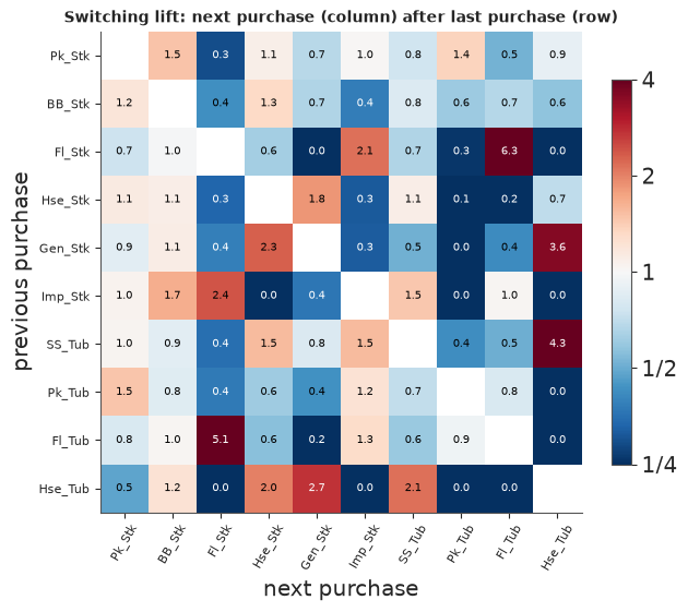
About half of all purchases repeat the previous one, and the switching that remains is far from proportional to shares. Blocks appear: Fleischmann's stick and tub swap buyers at five to six times the proportional rate; the house brand, the generic and Shedd's Spread form a cheap cluster; Parkay stick, Blue Bonnet and Parkay tub trade among themselves. Stick-versus-tub does not look like the organising principle.
But a switching matrix mixes three different things, and the market-structure argument needs only one of them:
- Heterogeneity. Different households like different products. A household that likes both Fleischmann's products alternates between them; aggregate switching then looks like substitution, and it is - but only for that kind of household.
- Prices. Promotions move buyers around; switching between two heavily promoted products is partly a record of the promotion calendar.
- State dependence. Buying a product may itself make the next purchase of it more likely (habit, learning, or just remembering where it is on the shelf). This inflates the diagonal and is a dynamic effect, not a statement about substitution.
And small cells are noisy: the house brand's tub was bought 33 times in all, so its row and column rest on a handful of switches. We need a model that separates the three and says how sure it is.
2 · The pooled logit
2.1 · Setup: training data and a held-out last purchase
We model each purchase as a choice among the 10 products (a household's first purchase is used only as the "previous purchase" of the second, because we will include state dependence). To compare models on data they have not seen, the last purchase of every household with at least three is held out; everything is fitted to the rest.
The utility of product $j$ for household $h$ on trip $t$ is
$$U_{htj} = \alpha_j + \beta\, p_{tj} + \gamma\, [\,j = \text{previous purchase}\,] + \varepsilon_{htj},$$
with Gumbel errors, so choice probabilities are a softmax (see E68 for the derivation). Parkay sticks are the reference ($\alpha_1 = 0$). The price prior Normal(-3, 2) per dollar is wide: a 10-cent price cut changes the odds of purchase by somewhere between -10% and +100%.
df["T"] = df.groupby("hh")["trip"].transform("max")
fit_rows = df[df["trip"] >= 2].copy()
fit_rows["test"] = (fit_rows["trip"] == fit_rows["T"]) & (fit_rows["T"] >= 3)
train, test = fit_rows[~fit_rows["test"]], fit_rows[fit_rows["test"]]


def arrays(d):
    return dict(X=d[[f"price_{p}" for p in PRODUCTS]].to_numpy(),
                last=np.eye(J)[d["prev"].astype(int).to_numpy()],
                y=d["y"].to_numpy(), hh=d["hh"].to_numpy())


tr, te = arrays(train), arrays(test)
print(f"training purchases {len(train):,}; held-out last purchases {len(test)}")
coords = {"product": PRODUCTS, "alt": PRODUCTS[1:]}


def logit_model(lag):
    with pm.Model(coords=coords) as m:
        a = pm.Normal("alpha", 0, 2, dims="alt")
        alpha = pt.concatenate([pt.zeros(1), a])
        beta = pm.Normal("beta", -3, 2)
        V = alpha + beta * tr["X"]
        if lag:
            V = V + pm.Normal("gamma", 0, 2) * tr["last"]
        pm.Categorical("y", logit_p=V, observed=tr["y"])
    return m


def fit(model, var_names=None):
    t0 = time.time()
    with model:
        idata = pm.sample(random_seed=RANDOM_SEED, var_names=var_names)
    ss = idata.sample_stats
    print(f"sampled in {time.time() - t0:.0f} s ({idata.posterior.attrs.get('tuning_steps')} warm-up "
          f"steps, nutpie); divergences {int(ss['diverging'].sum())}; max tree depth "
          f"{int(ss['depth'].max())}")
    return idata


idata_logit = fit(logit_model(lag=False))
idata_logit_lag = fit(logit_model(lag=True))
az.summary(idata_logit_lag, var_names=["alpha", "beta", "gamma"], round_to=2)
training purchases 3,498; held-out last purchases 456
sampled in 5 s (400 warm-up steps, nutpie); divergences 0; max tree depth 4
sampled in 3 s (400 warm-up steps, nutpie); divergences 0; max tree depth 4
| mean | sd | eti89_lb | eti89_ub | ess_bulk | ess_tail | r_hat | mcse_mean | mcse_sd | |
|---|---|---|---|---|---|---|---|---|---|
| alpha[BB_Stk] | -0.64 | 0.06 | -0.74 | -0.54 | 4941.04 | 3548.34 | 1.00 | 0.00 | 0.0 |
| alpha[Fl_Stk] | 2.22 | 0.13 | 2.01 | 2.44 | 928.53 | 1290.97 | 1.00 | 0.00 | 0.0 |
| alpha[Hse_Stk] | -1.36 | 0.07 | -1.46 | -1.25 | 3708.89 | 3128.64 | 1.00 | 0.00 | 0.0 |
| alpha[Gen_Stk] | -2.56 | 0.08 | -2.70 | -2.43 | 2474.97 | 2867.83 | 1.00 | 0.00 | 0.0 |
| alpha[Imp_Stk] | -0.58 | 0.15 | -0.82 | -0.35 | 3422.88 | 2870.53 | 1.00 | 0.00 | 0.0 |
| alpha[SS_Tub] | 0.88 | 0.10 | 0.72 | 1.04 | 1313.02 | 1695.48 | 1.00 | 0.00 | 0.0 |
| alpha[Pk_Tub] | 2.51 | 0.15 | 2.28 | 2.75 | 927.53 | 1315.30 | 1.00 | 0.00 | 0.0 |
| alpha[Fl_Tub] | 3.45 | 0.17 | 3.19 | 3.72 | 827.64 | 1234.27 | 1.01 | 0.01 | 0.0 |
| alpha[Hse_Tub] | -3.17 | 0.21 | -3.51 | -2.85 | 6261.90 | 3073.50 | 1.00 | 0.00 | 0.0 |
| beta | -7.45 | 0.21 | -7.80 | -7.11 | 777.90 | 1106.92 | 1.01 | 0.01 | 0.0 |
| gamma | 1.79 | 0.04 | 1.73 | 1.86 | 2936.72 | 2359.05 | 1.00 | 0.00 | 0.0 |
Clean fits in seconds. Price matters (about -7 per dollar per pound), and the pooled model says buying a product last time multiplies the odds of buying it again by $e^{1.8} \approx 6$. Hold that number; section 5 takes it apart.
2.2 · The logit has no market structure
Market structure is about substitution: when the price of $k$ goes up, where do its buyers go? The standard summary is the diversion ratio - of the purchases $k$ loses to a small price rise, the fraction that go to $j$:
$$D_{k \to j} = \frac{\partial s_j / \partial p_k}{-\,\partial s_k / \partial p_k}.$$
For the logit, $\partial s_j/\partial p_k = -\beta s_j s_k$ and $\partial s_k/\partial p_k = \beta s_k(1-s_k)$, so $D_{k\to j} = s_j / (1 - s_k)$: every product loses buyers to every other product in proportion to its size. This is IIA (independence of irrelevant alternatives) seen from the substitution side. Whatever the data say, the model's "diversion lift" - the diversion ratio divided by $s_j/(1-s_k)$, the counterpart of the switching lift - is exactly 1 everywhere. The logit cannot represent a submarket.
We will compute diversion ratios for every model the same way, as a population average of household-level derivatives at the median shelf prices, with the previous purchase switched off (a shopper with no history, so that the dynamic effect does not masquerade as substitution):
p_med = np.median(price, axis=0)


def diversion(A, b, prices=p_med):
    """Shares, diversion ratios D[s, j, k] (from k to j) and own-price elasticities.

    A: (S, H, J) household intercepts (H = 1 for a pooled model); b: (S, H) price coefficients.
    """
    Pr = special.softmax(A + b[..., None] * prices, axis=-1)
    s = Pr.mean(1)
    cross = -np.einsum("sh,shj,shk->sjk", b, Pr, Pr) / Pr.shape[1]    # d s_j / d p_k, j != k
    own = np.einsum("sh,shk->sk", b, Pr * (1 - Pr)) / Pr.shape[1]     # d s_k / d p_k (< 0)
    D = cross / -own[:, None, :]
    idx = np.arange(A.shape[-1])
    D[:, idx, idx] = np.nan
    return s, D, -own * prices / s


def pooled_params(idata, thin=4):
    p = az.extract(idata, var_names=["alpha", "beta"]).isel(sample=slice(None, None, thin))
    a = p["alpha"].transpose("sample", ...).to_numpy()
    A = np.concatenate([np.zeros((len(a), 1)), a], axis=1)[:, None, :]
    return A, p["beta"].to_numpy()[:, None]


s_logit, D_logit, el_logit = diversion(*pooled_params(idata_logit))
lift_logit = D_logit / (s_logit[:, :, None] / (1 - s_logit[:, None, :]))
print(f"logit diversion lift: min {np.nanmin(lift_logit):.6f}, max {np.nanmax(lift_logit):.6f}")
print("own-price elasticities (posterior median):",
      dict(zip(PRODUCTS, np.round(np.median(el_logit, 0), 1))))
logit diversion lift: min 1.000000, max 1.000000
own-price elasticities (posterior median): {'Pk_Stk': np.float64(2.5), 'BB_Stk': np.float64(3.2), 'Fl_Stk': np.float64(5.9), 'Hse_Stk': np.float64(2.4), 'Gen_Stk': np.float64(1.9), 'Imp_Stk': np.float64(4.7), 'SS_Tub': np.float64(5.1), 'Pk_Tub': np.float64(6.6), 'Fl_Tub': np.float64(7.2), 'Hse_Tub': np.float64(3.8)}
Exactly 1, as the algebra said. The own-price elasticities show a second artefact: in the logit the elasticity is $-\beta p_k (1 - s_k)$, proportional to price, so the expensive tubs come out as the most price-sensitive products (Parkay and Fleischmann's tubs: 6.6 and 7.2, against 2.5 for Parkay sticks) simply because they are expensive. Premium products are usually thought of as the opposite.
3 · The classic test: competing hierarchies as nested logits
The textbook way to add structure is the nested logit: group the products into nests, and let products in the same nest share a correlated error. A nest parameter $\lambda \in (0, 1]$ measures how much: $\lambda = 1$ is the plain logit, and as $\lambda \to 0$ products in a nest become perfect substitutes for each other. With nests $g$ and $S_g = \sum_{i \in g} e^{V_i/\lambda}$,
$$\log P(j) = \frac{V_j}{\lambda} + (\lambda - 1) \log S_{g(j)} - \log \sum_{g'} S_{g'}^{\lambda}.$$
Each hypothesis about the market is a partition; the test is which partition fits better. We try three:
- form first: sticks {6 products} vs tubs {4};
- brand first: {Parkay stick, Parkay tub}, {Fleischmann's stick, tub}, {house stick, tub}, and the four single-product brands on their own;
- quality tier (suggested by the switching matrix): mainstream {Parkay stick, Blue Bonnet, Parkay tub}, premium {Fleischmann's stick and tub, Imperial}, value {house stick, generic, Shedd's, house tub}.
The third was chosen after looking at the switching matrix - of the whole data set - so it has an
unfair advantage; keep that in mind. One shared $\lambda$ per model, prior Beta(2, 1.5) (mean 0.57,
plenty of mass near 1). The log-probability above is already normalised, so it can be passed to
pm.Categorical as logit_p directly.
PARTITIONS = {
    "form": [["Pk_Stk", "BB_Stk", "Fl_Stk", "Hse_Stk", "Gen_Stk", "Imp_Stk"],
             ["SS_Tub", "Pk_Tub", "Fl_Tub", "Hse_Tub"]],
    "brand": [["Pk_Stk", "Pk_Tub"], ["Fl_Stk", "Fl_Tub"], ["Hse_Stk", "Hse_Tub"], ["BB_Stk"],
              ["Gen_Stk"], ["Imp_Stk"], ["SS_Tub"]],
    "tier": [["Pk_Stk", "BB_Stk", "Pk_Tub"], ["Fl_Stk", "Fl_Tub", "Imp_Stk"],
             ["Hse_Stk", "Gen_Stk", "SS_Tub", "Hse_Tub"]],
}


def nest_arrays(part):
    groups = PARTITIONS[part]
    M = np.zeros((J, len(groups)))
    for g, members in enumerate(groups):
        M[[PRODUCTS.index(p) for p in members], g] = 1
    return M, M.argmax(1), np.array([len(g) > 1 for g in groups])


def nested_logp(V, lam1, M, gj, multi, xp=pt):
    """log P for a nested logit with one shared lambda (singleton nests have lambda = 1).

    Works for PyTensor (V: (n, J), lam1 scalar) and NumPy (V: (S, n, J), lam1: (S,))."""
    if xp is pt:
        lam = pt.switch(multi, lam1, 1.0)
        W = V[:, :, None] / lam + np.where(M > 0, 0.0, -1e9)
        logS = pt.logsumexp(W, axis=1)
        return (V / lam[gj] + (lam[gj] - 1) * logS[:, gj]
                - pt.logsumexp(lam * logS, axis=1, keepdims=True))
    lam = np.where(multi, lam1[:, None], 1.0)[:, None, :]              # (S, 1, G)
    W = V[..., None] / lam[:, :, None, :] + np.where(M > 0, 0.0, -1e9)
    logS = special.logsumexp(W, axis=2)                                 # (S, n, G)
    return (V / lam[..., gj] + (lam[..., gj] - 1) * logS[..., gj]
            - special.logsumexp(lam * logS, axis=2, keepdims=True))


def nested_model(part):
    M, gj, multi = nest_arrays(part)
    with pm.Model(coords=coords) as m:
        a = pm.Normal("alpha", 0, 2, dims="alt")
        alpha = pt.concatenate([pt.zeros(1), a])
        beta = pm.Normal("beta", -3, 2)
        lam = pm.Beta("lam", 2, 1.5)
        logp = nested_logp(alpha + beta * tr["X"], lam, M, gj, multi)
        pm.Categorical("y", logit_p=logp, observed=tr["y"])
    return m


idata_nested = {part: fit(nested_model(part)) for part in PARTITIONS}
pd.DataFrame({part: az.summary(idata, var_names=["lam", "beta"], round_to=2)[["mean", "sd", "eti89_lb",
                                                                               "eti89_ub", "r_hat"]].stack()
              for part, idata in idata_nested.items()}).unstack(0).round(2)
sampled in 21 s (400 warm-up steps, nutpie); divergences 0; max tree depth 5
sampled in 40 s (400 warm-up steps, nutpie); divergences 1; max tree depth 5
sampled in 28 s (400 warm-up steps, nutpie); divergences 0; max tree depth 5
| form | brand | tier | ||||
|---|---|---|---|---|---|---|
| lam | beta | lam | beta | lam | beta | |
| mean | 0.70 | -4.81 | 0.95 | -6.35 | 0.66 | -4.95 |
| sd | 0.07 | 0.45 | 0.04 | 0.20 | 0.05 | 0.31 |
| eti89_lb | 0.59 | -5.52 | 0.88 | -6.68 | 0.58 | -5.44 |
| eti89_ub | 0.82 | -4.09 | 0.99 | -6.02 | 0.74 | -4.47 |
| r_hat | 1.01 | 1.01 | 1.00 | 1.00 | 1.01 | 1.01 |
3.1 · Scoring on held-out purchases
Each held-out purchase is scored by its log predictive density, $\log \frac{1}{S}\sum_s p(y_{\text{test}} \mid \theta_s)$, summed over the 456 households (elpd; higher is better). The difference between two models is summed over the same purchases, so its standard error comes from the per-purchase differences, as in LOO.
def elpd_pointwise(logp_draws, y):
    """(S, n, J) log choice probabilities -> pointwise log predictive density (n,)."""
    ll = logp_draws[:, np.arange(len(y)), y]
    return special.logsumexp(ll, axis=0) - np.log(ll.shape[0])


def score_pooled(idata, nest=None, thin=4):
    A, b = pooled_params(idata, thin)
    V = A + b[:, :, None] * te["X"][None]
    if "gamma" in idata.posterior:
        g = az.extract(idata, var_names="gamma").to_numpy()[::thin]
        V = V + g[:, None, None] * te["last"][None]
    if nest is None:
        return elpd_pointwise(V - special.logsumexp(V, -1, keepdims=True), te["y"])
    lam = az.extract(idata, var_names="lam").to_numpy()[::thin]
    logp = np.concatenate([nested_logp(V[i:i + 100], lam[i:i + 100], *nest_arrays(nest), xp=np)
                           for i in range(0, len(lam), 100)])       # in chunks: (S, n, J, G) is big
    return elpd_pointwise(logp, te["y"])


scores = {"logit": score_pooled(idata_logit), "logit + last purchase": score_pooled(idata_logit_lag)}
scores |= {f"nested: {part}": score_pooled(idata, part) for part, idata in idata_nested.items()}


def score_table(scores, base="logit"):
    rows = []
    for name, s in scores.items():
        d = s - scores[base]
        rows.append(dict(model=name, elpd=s.sum(), diff=d.sum(), se_diff=d.std() * np.sqrt(len(d))))
    return pd.DataFrame(rows).set_index("model").round(1)


score_table(scores)
| elpd | diff | se_diff | |
|---|---|---|---|
| model | |||
| logit | -644.9 | 0.0 | 0.0 |
| logit + last purchase | -561.2 | 83.7 | 17.2 |
| nested: form | -639.6 | 5.3 | 1.7 |
| nested: brand | -645.4 | -0.5 | 0.2 |
| nested: tier | -641.6 | 3.3 | 2.3 |
Read the table in two parts.
The nest parameters. Form and tier both get $\lambda$ well below 1 (about 0.7), which on its own looks like strong evidence for a hierarchy; the brand partition's $\lambda$ sits near 1. A classic analysis would conclude "form first, not brand first", and the tier partition, fitted after peeking, looks as good.
The held-out scores. None of them beats the plain logit by more than about two standard errors on 456 purchases, and they are indistinguishable from each other. Adding the last purchase is worth far more than any nesting.
The deeper problem is what $\lambda < 1$ means in pooled data. A nested logit's correlated error is meant to be a within-trip taste shock shared by similar products. But pooled across 516 households, persistent differences between households (one family always buys cheap margarine, another always Fleischmann's) also make products "correlated", and any partition that roughly groups the products that the same households buy will soak some of it up. The test cannot distinguish "these products substitute for each other on a trip" from "these products are bought by the same people", and it only compares hypotheses we thought of. We need to model the households.
4 · A choice map
4.1 · Household heterogeneity with a factor structure
Give every household its own brand intercepts and price sensitivity:
$$U_{htj} = \alpha_j + \boldsymbol{\lambda}_j^\top \mathbf{z}_h + \sigma\, e_{hj} + \beta_h\, p_{tj} + \gamma\,[\,j = \text{previous}\,] + \varepsilon_{htj},$$
- $\mathbf{z}_h \sim N(0, I_K)$ is household $h$'s position in a $K$-dimensional taste space;
- $\boldsymbol{\lambda}_j$ is product $j$'s loading - a direction in that space. A household likes product $j$ in proportion to how far it lies along $\boldsymbol{\lambda}_j$. This is the vector model of Elrod (1988) and Elrod & Keane (1995), fitted as a factor-analytic random-effects logit;
- $e_{hj} \sim N(0, 1)$ is a product-specific idiosyncratic taste not explained by the map;
- $\beta_h = -\exp(\mu_b + \sigma_b u_h)$: everybody dislikes paying more, by an amount that varies (the lognormal lesson of E68).
The household intercepts then have covariance $\Lambda \Lambda^\top + \sigma^2 I$. Two products whose loading vectors point the same way are liked by the same households, so they draw on the same pool of buyers: when one gets dearer, its buyers move to the other. That is the market structure, and the $K = 2$ version can be drawn as a map.
Two technical points. Adding the same constant to every product's utility changes nothing, so the loadings are centred across products (each column of $\Lambda$ sums to zero), which removes the unidentified "likes margarine" direction. And the loadings get a Normal(0, 1.5) prior, the idiosyncratic scale $\sigma$ a HalfNormal(1).
def choice_map(K, idiosyncratic=True, lag=True):
    c = coords | {"hh": np.arange(H), "dim": np.arange(K)}
    with pm.Model(coords=c) as m:
        a = pm.Normal("alpha", 0, 2, dims="alt")
        alpha = pt.concatenate([pt.zeros(1), a])
        raw = pm.Normal("raw_loadings", 0, 1.5, dims=("product", "dim"))
        Lam = pm.Deterministic("Lambda", raw - raw.mean(axis=0), dims=("product", "dim"))
        z = pm.Normal("z", 0, 1, dims=("hh", "dim"))
        A = alpha + z @ Lam.T
        if idiosyncratic:
            sigma = pm.HalfNormal("sigma", 1.0)
            A = A + sigma * pm.Normal("e", 0, 1, dims=("hh", "product"))
        mu_b = pm.Normal("mu_b", 1.0, 1.0)
        sd_b = pm.HalfNormal("sd_b", 1.0)
        u = pm.Normal("u", 0, 1, dims="hh")
        b = -pt.exp(mu_b + sd_b * u)
        V = A[tr["hh"]] + b[tr["hh"], None] * tr["X"]
        if lag:
            V = V + pm.Normal("gamma", 0, 2) * tr["last"]
        pm.Categorical("y", logit_p=V, observed=tr["y"])
    return m


m_map2 = choice_map(K=2)
4.2 · Prior predictive check
Are the priors sensible? Households in the data are fairly loyal: among households with at least three training purchases, the median one puts 60% of them on its favourite product. Simulate choices under the prior and compute the same statistic.
def favourite_share(y, hh):
    t = pd.crosstab(hh, y)
    return (t.max(axis=1) / t.sum(axis=1))[t.sum(axis=1) >= 3]


with m_map2:
    prior = pm.sample_prior_predictive(draws=200, random_seed=RANDOM_SEED)
y_prior = prior.prior_predictive["y"].to_numpy().reshape(200, -1)
fav_prior = [favourite_share(y_prior[i], tr["hh"]).median() for i in range(200)]
fav_obs = favourite_share(tr["y"], tr["hh"]).median()
print(f"observed median favourite share {fav_obs:.2f}; prior predictive 5-50-95%: {q(fav_prior)}")
print(f"prior median price coefficient exp(mu_b), 5-95%: {q(np.exp(prior.prior['mu_b']), (0.05, 0.95))}")
observed median favourite share 0.60; prior predictive 5-50-95%: [0.55 0.67 0.89]
prior median price coefficient exp(mu_b), 5-95%: [ 0.51 15.18]
The prior allows anything from promiscuous to loyal households and puts the observed value comfortably inside; the price coefficient ranges over two orders of magnitude. Nothing is forced.
4.3 · Fit - and a map that will not converge
KEEP = ["alpha", "Lambda", "z", "sigma", "e", "mu_b", "sd_b", "u", "gamma"]
idata_map2 = fit(m_map2, var_names=KEEP)
summ = az.summary(idata_map2, var_names=["mu_b", "sd_b", "sigma", "gamma", "Lambda"], round_to=2)
summ.iloc[:10]
sampled in 18 s (400 warm-up steps, nutpie); divergences 0; max tree depth 5
| mean | sd | eti89_lb | eti89_ub | ess_bulk | ess_tail | r_hat | mcse_mean | mcse_sd | |
|---|---|---|---|---|---|---|---|---|---|
| mu_b | 2.22 | 0.04 | 2.14 | 2.29 | 751.09 | 1066.57 | 1.00 | 0.00 | 0.00 |
| sd_b | 0.43 | 0.04 | 0.36 | 0.49 | 575.42 | 1047.82 | 1.01 | 0.00 | 0.00 |
| sigma | 1.19 | 0.07 | 1.08 | 1.32 | 407.51 | 835.77 | 1.01 | 0.00 | 0.00 |
| gamma | 0.36 | 0.06 | 0.26 | 0.45 | 1988.78 | 2340.62 | 1.00 | 0.00 | 0.00 |
| Lambda[Pk_Stk, 0] | 0.38 | 0.74 | -1.02 | 1.31 | 6.45 | 7.85 | 1.66 | 0.30 | 0.15 |
| Lambda[Pk_Stk, 1] | 0.73 | 0.53 | -0.27 | 1.42 | 9.54 | 11.23 | 1.34 | 0.19 | 0.09 |
| Lambda[BB_Stk, 0] | 0.21 | 0.47 | -0.61 | 0.87 | 7.49 | 10.29 | 1.49 | 0.18 | 0.07 |
| Lambda[BB_Stk, 1] | 0.43 | 0.36 | -0.22 | 0.94 | 12.77 | 17.41 | 1.22 | 0.11 | 0.04 |
| Lambda[Fl_Stk, 0] | -2.01 | 1.10 | -3.28 | 0.35 | 11.79 | 8.77 | 1.26 | 0.37 | 0.29 |
| Lambda[Fl_Stk, 1] | -0.33 | 1.89 | -2.92 | 2.71 | 6.17 | 12.53 | 1.72 | 0.78 | 0.25 |
print(f"r_hat, all scalars: max {summ.loc[['mu_b', 'sd_b', 'sigma', 'gamma'], 'r_hat'].max():.2f}; "
      f"loadings: {summ.filter(like='Lambda', axis=0)['r_hat'].min():.2f}-"
      f"{summ.filter(like='Lambda', axis=0)['r_hat'].max():.2f}, bulk ESS as low as "
      f"{summ.filter(like='Lambda', axis=0)['ess_bulk'].min():.0f}")
r_hat, all scalars: max 1.01; loadings: 1.14-1.79, bulk ESS as low as 6
No divergences, and the scalar parameters are fine. The loadings are a disaster by the usual rules: r_hat up to 1.8 and single-digit effective sample sizes. Let us look before we "fix" anything: each chain's draws of the ten loading vectors, one colour per chain.
Lam_draws = idata_map2.posterior["Lambda"].to_numpy()          # (chain, draw, product, dim)
show = {"Fl_Stk": BLUE, "Hse_Tub": ORANGE, "Pk_Tub": AQUA}
fig, axes = plt.subplots(1, 4, figsize=(14, 4), sharex=True, sharey=True)
for c, ax in enumerate(axes):
    for j, p in enumerate(PRODUCTS):
        ax.scatter(*Lam_draws[c, ::4, j].T, s=2, alpha=0.4 if p in show else 0.15,
                   color=show.get(p, GREY), label=p if p in show and c == 0 else None)
    ax.set_title(f"chain {c}")
    ax.set_aspect("equal")
axes[0].legend(fontsize=7, markerscale=4, loc="lower left")
fig.suptitle("Raw draws of the loadings (three products coloured, the rest grey)");
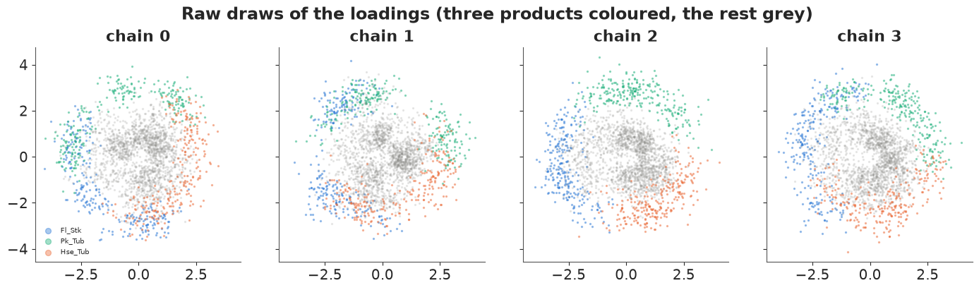
Each product's draws stay at roughly the same distance from the origin, and the three coloured products keep roughly the same angles to each other, but the configuration as a whole wanders around the circle: draws are smeared along arcs within a chain, and chains disagree about where on the circle the map sits. That is not a sampling failure. The likelihood depends on the loadings only through $\boldsymbol{\lambda}_j^\top \mathbf{z}_h$, and for any rotation $R$, $(\Lambda R)(R^\top \mathbf{z}_h) = \Lambda \mathbf{z}_h$, while the prior on $\mathbf{z}_h$ is rotation-invariant. The posterior is a ring of equivalent maps. r_hat is right to complain that the chains disagree about $\Lambda$ - $\Lambda$ is not identified - but everything we actually want is:
- the covariance $\Lambda\Lambda^\top$ (how much the same households like two products) is invariant to $R$;
- so are the choice probabilities, diversion ratios and elasticities.
LLt = xr.DataArray(np.einsum("cdjk,cdik->cdji", Lam_draws, Lam_draws), dims=("chain", "draw", "j", "i"))
print(f"Lambda Lambda^T: r_hat max {float(az.rhat(LLt).max()):.3f}, "
      f"bulk ESS min {float(az.ess(LLt).min()):.0f}")
Lambda Lambda^T: r_hat max 1.034, bulk ESS min 155
The identified quantity has converged. Two standard ways out for the map: constrain $\Lambda$ (e.g. lower-triangular with a positive diagonal, which pins the first axis to one "anchor" product and can create new multimodality if that anchor's true loading is near zero), or leave the sampler alone and align the draws afterwards. We do the second: an orthogonal Procrustes rotation of every draw onto a common reference (generalised Procrustes: align to one draw, average, realign to the average, repeat). Rotations and reflections are allowed, stretching is not, so relative distances and angles - the map's content - are untouched. Households' positions are rotated by the same matrix.
def procrustes_align(L, iters=5):
    """Rotate (orthogonally) every draw of L (S, J, K) onto a common reference; returns L R, R."""
    ref = L[0]
    for _ in range(iters):
        U, _, Vt = np.linalg.svd(np.einsum("sjk,jl->skl", L, ref))
        R = U @ Vt
        ref = np.einsum("sjk,skl->jl", L, R) / len(L)
    # final orientation: principal axes of the mean map, Fleischmann's stick on the positive side
    _, _, Vt = np.linalg.svd(ref, full_matrices=False)
    flip = np.sign((ref @ Vt.T)[PRODUCTS.index("Fl_Stk")])
    R = R @ Vt.T * flip
    return np.einsum("sjk,skl->sjl", L, R), R


def aligned_map(idata):
    L = idata.posterior["Lambda"].to_numpy()
    C, S = L.shape[:2]
    L_al, R = procrustes_align(L.reshape(C * S, J, -1))
    z = idata.posterior["z"].to_numpy().reshape(C * S, H, -1)
    return L_al.reshape(C, S, J, -1), np.einsum("shk,skl->shl", z, R).reshape(C, S, H, -1)


Lam_al, z_al = aligned_map(idata_map2)
r_al = az.rhat(xr.DataArray(Lam_al, dims=("chain", "draw", "product", "dim")))
print(f"aligned loadings: r_hat {float(r_al.min()):.3f}-{float(r_al.max()):.3f}")
aligned loadings: r_hat 1.002-1.042
After alignment r_hat is at most about 1.04 - above the usual 1.01 threshold, but the same slow mixing that the identified $\Lambda\Lambda^\top$ showed, not chains in different places. The map can now be drawn with honest uncertainty: each product's loading with a 90% posterior ellipse, and the posterior mean position of every household behind it.
def draw_map(ax, L, z, title):
    Lf = L.reshape(-1, J, L.shape[-1])
    zm = z.reshape(-1, H, z.shape[-1]).mean(0)
    ax.scatter(*zm.T, s=6, color=GREY, alpha=0.35, label="households (posterior mean z)")
    for j, p in enumerate(PRODUCTS):
        m = Lf[:, j].mean(0)
        cov = np.cov(Lf[:, j].T)
        vals, vecs = np.linalg.eigh(cov)
        ang = np.degrees(np.arctan2(vecs[1, 1], vecs[0, 1]))
        colr = BLUE if p.endswith("Stk") else ORANGE
        ax.add_patch(Ellipse(m, *(2 * np.sqrt(vals[::-1] * 4.6)), angle=ang, color=colr, alpha=0.18))
        ax.annotate("", m, (0, 0), arrowprops=dict(arrowstyle="-|>", color=colr, lw=1.4))
        ax.annotate(p, m, xytext=(4, 4), textcoords="offset points", fontsize=9, color=colr,
                    fontweight="bold")
    ax.axhline(0, color=GREY, lw=0.5)
    ax.axvline(0, color=GREY, lw=0.5)
    ax.set_aspect("equal")
    ax.set_xlabel("taste dimension 1")
    ax.set_ylabel("taste dimension 2")
    ax.set_title(title)


fig, ax = plt.subplots(figsize=(8, 7.5))
draw_map(ax, Lam_al, z_al, "Choice map: product loadings (arrows, 90% ellipses) and households")
ax.legend(loc="lower left", fontsize=8);
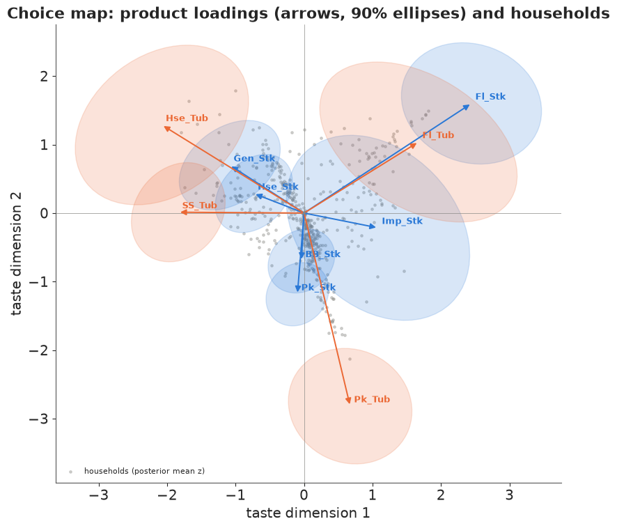
How to read it: a household at position $\mathbf{z}$ gets a utility bonus $\boldsymbol\lambda_j^\top \mathbf{z}$ for product $j$ - large when it lies far out in the direction of $j$'s arrow. Products whose arrows point the same way appeal to the same households and are close substitutes; products pointing in opposite directions split the households between them. Long arrows are polarising (strong likes and dislikes); short arrows, like Parkay and Blue Bonnet sticks, are products whose appeal differs little between households, and their buyers are drawn from everywhere.
Three directions stand out, and they are neither "form" nor "brand":
- Premium: Fleischmann's stick and tub point the same way, with Imperial (short, uncertain) roughly along. Fleischmann's buyers are a distinct group that buys that brand in either form.
- Value: the house brand (stick and tub), the generic and Shedd's Spread point roughly the opposite way - households that buy on price.
- Mainstream: Parkay tub has a long arrow of its own, pointing roughly where the short Parkay and Blue Bonnet stick arrows point. Those two sticks sit near the centre: their buyers come from everywhere.
This is the quality-tier structure Allenby & Rossi (1991) described for these data.
5 · How many dimensions, and is loyalty real?
Fit one- and three-dimensional maps, a two-dimensional map without the idiosyncratic term $\sigma e_{hj}$, and score them all on the held-out last purchases. For a map the prediction for a household uses its posterior $\mathbf{z}_h$, $e_h$ and $\beta_h$, which is exactly what "predict this household's next purchase" should mean.
def household_params(idata, thin=4):
    """Per-draw household intercepts A (S, H, J), price coefficients b (S, H), gamma (S,)."""
    p = idata.posterior.isel(draw=slice(None, None, thin))
    S = p.sizes["chain"] * p.sizes["draw"]
    alpha = np.concatenate([np.zeros((S, 1)), p["alpha"].to_numpy().reshape(S, -1)], axis=1)
    Lam = p["Lambda"].to_numpy().reshape(S, J, -1)
    A = alpha[:, None, :] + np.einsum("shk,sjk->shj", p["z"].to_numpy().reshape(S, H, -1), Lam)
    if "sigma" in p:
        A = A + p["sigma"].to_numpy().reshape(S)[:, None, None] * p["e"].to_numpy().reshape(S, H, J)
    b = -np.exp(p["mu_b"].to_numpy().reshape(S)[:, None]
                + p["sd_b"].to_numpy().reshape(S)[:, None] * p["u"].to_numpy().reshape(S, H))
    g = p["gamma"].to_numpy().reshape(S) if "gamma" in p else np.zeros(S)
    return A, b, g


def score_map(idata):
    A, b, g = household_params(idata)
    V = A[:, te["hh"]] + b[:, te["hh"], None] * te["X"] + g[:, None, None] * te["last"]
    return elpd_pointwise(V - special.logsumexp(V, -1, keepdims=True), te["y"])


idata_maps = {"map K=2": idata_map2}
for name, kw in [("map K=1", dict(K=1)), ("map K=3", dict(K=3)),
                 ("map K=2, no idiosyncratic", dict(K=2, idiosyncratic=False))]:
    idata_maps[name] = fit(choice_map(**kw), var_names=[v for v in KEEP if v not in ("sigma", "e")
                                                        or kw.get("idiosyncratic", True)])
scores |= {name: score_map(idata) for name, idata in idata_maps.items()}
gammas = {name: az.extract(idata, var_names="gamma").to_numpy() for name, idata in idata_maps.items()}
_s, _D, _ = diversion(*household_params(idata_maps["map K=3"], thin=10)[:2])
lift_k3 = np.nanmedian(_D / (_s[:, :, None] / (1 - _s[:, None, :])), 0)   # for section 7
for name in list(idata_maps):
    if name != "map K=2":
        del idata_maps[name]                       # keep memory down: only their gammas are needed now
print(score_table({k: v for k, v in scores.items() if k.startswith("map")}, base="map K=2"), "\n")
score_table(scores)
sampled in 18 s (400 warm-up steps, nutpie); divergences 0; max tree depth 5
sampled in 19 s (400 warm-up steps, nutpie); divergences 0; max tree depth 5
sampled in 17 s (400 warm-up steps, nutpie); divergences 0; max tree depth 5
                            elpd  diff  se_diff
model
map K=2                   -391.1   0.0      0.0
map K=1                   -398.6  -7.5      2.8
map K=3                   -386.2   4.9      1.7
map K=2, no idiosyncratic -405.4 -14.4      5.7
| elpd | diff | se_diff | |
|---|---|---|---|
| model | |||
| logit | -644.9 | 0.0 | 0.0 |
| logit + last purchase | -561.2 | 83.7 | 17.2 |
| nested: form | -639.6 | 5.3 | 1.7 |
| nested: brand | -645.4 | -0.5 | 0.2 |
| nested: tier | -641.6 | 3.3 | 2.3 |
| map K=2 | -391.1 | 253.8 | 22.9 |
| map K=1 | -398.6 | 246.3 | 22.7 |
| map K=3 | -386.2 | 258.7 | 22.8 |
| map K=2, no idiosyncratic | -405.4 | 239.5 | 22.0 |
Modelling households is worth about 250 nats on 456 held-out purchases - more than half a nat per purchase, a 1.7-fold gain in the probability given to what the household actually bought. Everything in section 3 was a rounding error by comparison.
Among the maps (first table, relative to K = 2): one dimension is worse by 7.5 $\pm$ 2.8, dropping the idiosyncratic term costs 14 $\pm$ 6, and a third dimension helps a little - 4.9 $\pm$ 1.7 nats, about 0.01 nats per purchase. That is a real but small gain. We keep K = 2 with the idiosyncratic term because the map can be drawn, and check in section 7 that the third dimension does not change the substitution patterns we report.
5.1 · Loyalty is mostly heterogeneity
Now look at $\gamma$, the effect of the previous purchase, across models:
gam = {"logit + last purchase": az.extract(idata_logit_lag, var_names="gamma").to_numpy()}
gam |= {k: gammas[k] for k in ["map K=2, no idiosyncratic", "map K=1", "map K=2", "map K=3"]}
fig, ax = plt.subplots(figsize=(8, 3))
for i, (name, g) in enumerate(gam.items()):
    lo, mid, hi = np.quantile(g, [0.05, 0.5, 0.95])
    ax.plot([lo, hi], [i, i], color=BLUE, lw=3)
    ax.plot(mid, i, "o", color=BLUE)
    ax.text(hi + 0.05, i, f"{mid:.2f}  (odds x{np.exp(mid):.1f})", va="center", fontsize=8)
ax.set_yticks(range(len(gam)), list(gam))
ax.set_xlabel(r"$\gamma$: log-odds bonus for last time's product (90% interval)")
ax.set_xlim(0, 2.4)
ax.set_title("Apparent state dependence shrinks as household heterogeneity is modelled");
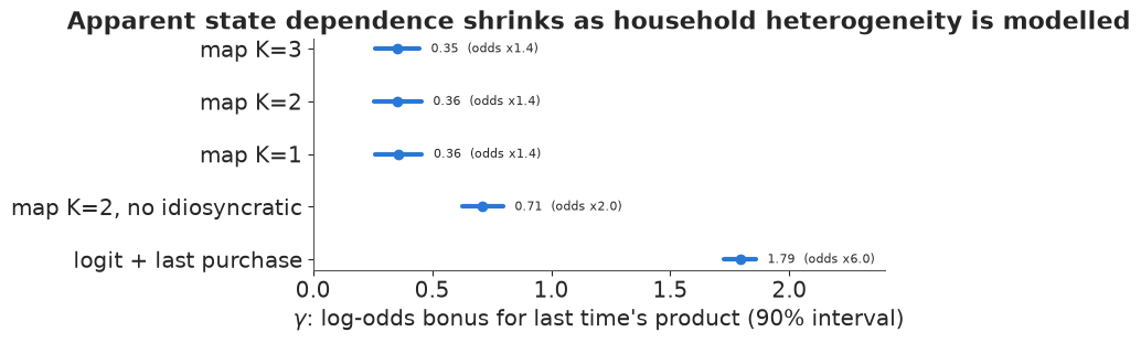
The pooled logit's "buying it last time multiplies the odds by 6" falls to 1.4 once households have their own tastes. Most of the apparent loyalty was spurious state dependence (Heckman 1981): households that bought Fleischmann's last time are Fleischmann's households, and they would have bought it again anyway. An incomplete model of heterogeneity (no idiosyncratic term) leaves some of it behind, which is how $\gamma$ is used in practice: as a diagnostic of whether the heterogeneity model is rich enough. Keane (1997) and Dubé, Hitsch & Rossi (2010) found the same pattern - genuine but modest state dependence - in other scanner panels.
For market structure this matters directly: a model that mistakes preference for habit will predict that a price cut wins "loyal" customers for a long time, and will read the switching matrix's blocks as dynamics rather than as who-competes-with-whom.
6 · Posterior predictive check: simulated purchase histories
Held-out scores judge one purchase per household. A market-structure model should also reproduce the patterns of switching. For posterior draws, we re-run every household's purchase history: start from its observed first purchase, and on each later trip draw the purchase from the model given that trip's prices and the simulated previous purchase. Then compute the statistics of section 1 on the simulated panel.
first = df[df["trip"] == 1].set_index("hh")["y"].reindex(range(H)).to_numpy()
T_max = df["trip"].max()
Xpad = np.zeros((H, T_max, J))
Xpad[df["hh"], df["trip"] - 1] = price
n_trips = df.groupby("hh").size().reindex(range(H)).to_numpy()


def simulate_panel(A, b, g, n_sims=100, seed=1):
    """Simulated histories (n_sims, H, T_max), -1 after a household's last trip."""
    r = np.random.default_rng(seed)
    idx = r.choice(len(b), n_sims, replace=False)
    Y = np.full((n_sims, H, T_max), -1)
    Y[:, :, 0] = first
    for t in range(1, T_max):
        V = A[idx] + b[idx][..., None] * Xpad[:, t] + g[idx, None, None] * np.eye(J)[Y[:, :, t - 1]]
        Pr = special.softmax(V, -1)
        draw = (Pr.cumsum(-1) > r.random(Pr.shape[:2])[..., None]).argmax(-1)
        Y[:, :, t] = np.where(t < n_trips, draw, -1)
    return Y


def panel_stats(Y):
    """Repeat rate, distinct products per household (share with 1, 2, 3+), switching lift."""
    prev, nxt = Y[:, :-1].ravel(), Y[:, 1:].ravel()
    ok = nxt >= 0
    sw = np.zeros((J, J))
    np.add.at(sw, (prev[ok], nxt[ok]), 1)
    counts = np.bincount(Y[Y >= 0], minlength=J)
    n_distinct = np.array([len(set(row[row >= 0])) for row in Y])
    return dict(repeat=np.trace(sw) / sw.sum(), lift=switching_lift(sw, counts / counts.sum()),
                distinct=np.array([(n_distinct == 1).mean(), (n_distinct == 2).mean(),
                                   (n_distinct >= 3).mean()]))


Y_obs = np.full((H, T_max), -1)
Y_obs[df["hh"], df["trip"] - 1] = df["y"]
obs_stats = panel_stats(Y_obs)
A_l, b_l = pooled_params(idata_logit_lag)
g_l = az.extract(idata_logit_lag, var_names="gamma").to_numpy()[::4]
sims = {"logit + last purchase": simulate_panel(np.repeat(A_l, H, 1), np.repeat(b_l, H, 1), g_l),
        "map K=2": simulate_panel(*household_params(idata_map2))}
sim_stats = {k: [panel_stats(Y) for Y in v] for k, v in sims.items()}
for k, st in sim_stats.items():
    print(f"{k:22s} repeat rate {q([s['repeat'] for s in st])} (observed {obs_stats['repeat']:.2f}); "
          f"households buying 1 / 2 / 3+ products: "
          f"{np.round(np.mean([s['distinct'] for s in st], 0), 2)} "
          f"(observed {np.round(obs_stats['distinct'], 2)})")
logit + last purchase  repeat rate [0.48 0.5  0.52] (observed 0.49); households buying 1 / 2 / 3+ products: [0.14 0.21 0.65] (observed [0.17 0.33 0.5 ])
map K=2                repeat rate [0.48 0.49 0.51] (observed 0.49); households buying 1 / 2 / 3+ products: [0.14 0.31 0.55] (observed [0.17 0.33 0.5 ])
fig, axes = plt.subplots(1, 3, figsize=(16, 5))
heat(axes[0], obs_stats["lift"], "Observed switching lift")
for ax, (k, st) in zip(axes[1:], sim_stats.items()):
    heat(ax, np.nanmedian([s["lift"] for s in st], 0), f"Simulated histories: {k}")
;
''
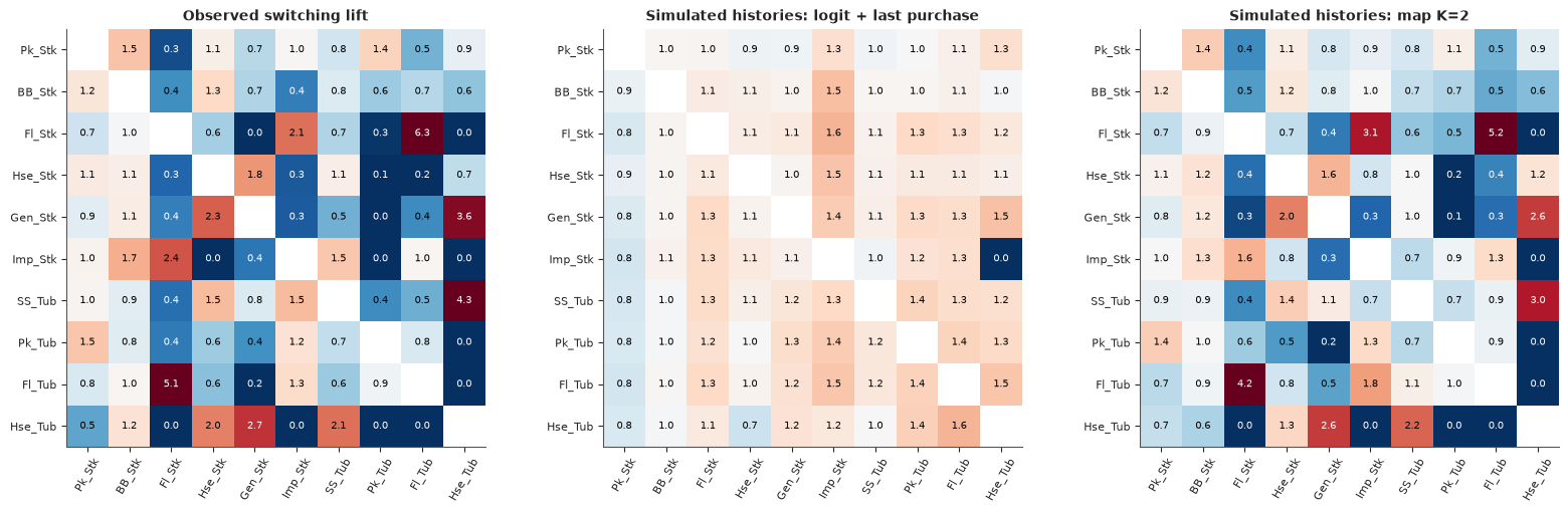
Both models get the overall repeat rate right (0.49), the pooled logit because that is what its $\gamma$ was fitted to do. Everything else separates them:
- Spread of households over products. Observed: 17% of households bought one product, 33% two, 50% three or more. The pooled logit gives 14 / 21 / 65% - it moves each household around the whole category. The map gives 14 / 31 / 55%, much closer though still slightly too promiscuous.
- Switching lift. The pooled logit's simulated lift is nearly flat (0.7-1.6, no blocks): every product exchanges buyers in proportion to its size. The map reproduces the blocks of the observed matrix - Fleischmann's stick and tub (5.2 and 4.2 simulated, 6.3 and 5.1 observed), the value group, Parkay stick with Blue Bonnet - even though it was fitted to individual choices, never to switching counts.
7 · Reading the market structure off the posterior
7.1 · Diversion lift
The counterpart of section 1's switching lift, now as a counterfactual: raise the price of $k$ a little, holding everything else fixed; where do its lost purchases go, relative to the logit's share-proportional answer? Computed per posterior draw from the households' parameters, with the previous purchase switched off.
A2, b2, _ = household_params(idata_map2, thin=10)
s_map, D_map, el_map = diversion(A2, b2)
lift_map = D_map / (s_map[:, :, None] / (1 - s_map[:, None, :]))
lift_med = np.nanmedian(lift_map, 0)
fig, axes = plt.subplots(1, 2, figsize=(13, 5.5))
heat(axes[0], lift_raw.T, "Observed switching lift (transposed: row = to, column = from)")
heat(axes[1], lift_med, "Choice map: diversion lift (row j receives from column k)")
;
''
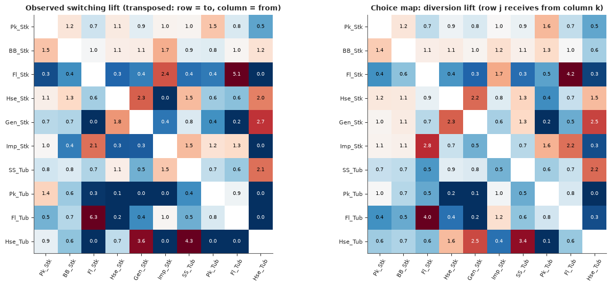
The model's diversion lift is a cleaned-up version of the switching lift: the same blocks, without the zeros and extreme ratios of the smallest cells, and with each number now meaning something definite (substitution after a price change, net of dynamics). The three-dimensional map (section 5) gives nearly the same matrix:
lk2, lk3 = np.log(lift_med), np.log(lift_k3)
ok = np.isfinite(lk2)
print(f"K=2 vs K=3 diversion lift: correlation of log lifts {np.corrcoef(lk2[ok], lk3[ok])[0, 1]:.2f}; "
      f"median |ratio - 1| {np.median(np.abs(np.exp(lk3[ok] - lk2[ok]) - 1)):.0%}")
K=2 vs K=3 diversion lift: correlation of log lifts 0.93; median |ratio - 1| 8%
How sure are we about the key pairs?
key_pairs = [("Fl_Stk", "Fl_Tub"), ("Fl_Tub", "Imp_Stk"), ("Hse_Stk", "Gen_Stk"), ("SS_Tub", "Hse_Tub"),
             ("Pk_Stk", "Pk_Tub"), ("Pk_Stk", "BB_Stk"), ("Pk_Stk", "SS_Tub"), ("Pk_Tub", "SS_Tub"),
             ("Fl_Stk", "Hse_Stk")]
rows = []
for k, j in key_pairs:
    ik, ij = PRODUCTS.index(k), PRODUCTS.index(j)
    x = lift_map[:, ij, ik]
    rows.append(dict(pair=f"{k} -> {j}", diversion=np.median(D_map[:, ij, ik]),
                     lift_5=np.quantile(x, 0.05), lift_50=np.median(x), lift_95=np.quantile(x, 0.95),
                     logit_diversion=np.median(D_logit[:, ij, ik])))
pd.DataFrame(rows).set_index("pair").round(2)
| diversion | lift_5 | lift_50 | lift_95 | logit_diversion | |
|---|---|---|---|---|---|
| pair | |||||
| Fl_Stk -> Fl_Tub | 0.22 | 3.06 | 4.01 | 5.11 | 0.07 |
| Fl_Tub -> Imp_Stk | 0.05 | 1.08 | 2.15 | 3.29 | 0.03 |
| Hse_Stk -> Gen_Stk | 0.26 | 2.02 | 2.30 | 2.60 | 0.12 |
| SS_Tub -> Hse_Tub | 0.03 | 2.03 | 3.43 | 5.27 | 0.01 |
| Pk_Stk -> Pk_Tub | 0.08 | 0.87 | 1.00 | 1.18 | 0.08 |
| Pk_Stk -> BB_Stk | 0.29 | 1.32 | 1.43 | 1.53 | 0.19 |
| Pk_Stk -> SS_Tub | 0.09 | 0.61 | 0.72 | 0.84 | 0.10 |
| Pk_Tub -> SS_Tub | 0.05 | 0.31 | 0.62 | 1.08 | 0.07 |
| Fl_Stk -> Hse_Stk | 0.15 | 0.65 | 0.90 | 1.15 | 0.16 |
A small rise in the price of Fleischmann's stick sends 22% of its lost purchases to Fleischmann's tub - four times the share-proportional rate (90% interval 3.1-5.1); the logit says 7%. The value pairs (house stick to generic, Shedd's to house tub) are two to three times proportional. But Parkay stick to Parkay tub is exactly proportional (lift 1.0, 0.87-1.18): Parkay buyers do not prefer the other Parkay form, so Fleischmann's is the only brand whose buyers cross forms. And the national-brand tubs lose fewer buyers to the cheap Shedd's tub than proportional (0.6). Form is not a submarket.
7.2 · A market tree, with uncertainty
A tree is the traditional display. Cluster the products using $1/\text{lift}$ as a dissimilarity (symmetrised; average linkage), per posterior draw, and record how often each group of products appears as a cluster - a Bayesian version of bootstrap support on a phylogeny.
def tree(lift):
    L = np.nan_to_num((lift + lift.T) / 2, nan=np.inf)
    dist = 1 / L
    np.fill_diagonal(dist, 0)
    return hierarchy.linkage(dist[np.triu_indices(J, 1)], method="average")


def clusters(Z):
    """The clusters of a linkage, in merge order (row n of Z creates clusters(Z)[n])."""
    out, members = [], {i: frozenset([i]) for i in range(J)}
    for n, (a, b, *_) in enumerate(Z):
        members[J + n] = members[int(a)] | members[int(b)]
        out.append(members[J + n])
    return out


Z_med = tree(lift_med)
draw_sets = [set(clusters(tree(lift_map[s]))) for s in range(len(lift_map))]
support = [np.mean([c in d for d in draw_sets]) for c in clusters(Z_med)]
fig, ax = plt.subplots(figsize=(9, 4.5))
dn = hierarchy.dendrogram(Z_med, labels=PRODUCTS, ax=ax, color_threshold=0, above_threshold_color=GREY)
# each merge is drawn as an upside-down U at its height; label the top centre of each U
tops = [(d[1], (i[1] + i[2]) / 2) for i, d in zip(dn["icoord"], dn["dcoord"])]
for n, (c, sup) in enumerate(zip(clusters(Z_med), support)):
    if len(c) < J:
        x = [xc for h, xc in tops if np.isclose(h, Z_med[n, 2])][0]
        ax.text(x, Z_med[n, 2] + 0.03, f"{sup:.0%}", ha="center", va="bottom", fontsize=8, color=RED)
        print(f"{sorted(PRODUCTS[i] for i in c)}: support {sup:.0%}")
ax.set_ylabel("1 / diversion lift (average linkage)")
ax.set_title("Market tree from the choice map; red: share of posterior draws with that cluster");
['Fl_Stk', 'Fl_Tub']: support 93%
['Hse_Tub', 'SS_Tub']: support 62%
['Gen_Stk', 'Hse_Stk']: support 64%
['Fl_Stk', 'Fl_Tub', 'Imp_Stk']: support 70%
['Gen_Stk', 'Hse_Stk', 'Hse_Tub', 'SS_Tub']: support 95%
['BB_Stk', 'Pk_Stk']: support 59%
['BB_Stk', 'Pk_Stk', 'Pk_Tub']: support 66%
['BB_Stk', 'Fl_Stk', 'Fl_Tub', 'Imp_Stk', 'Pk_Stk', 'Pk_Tub']: support 84%
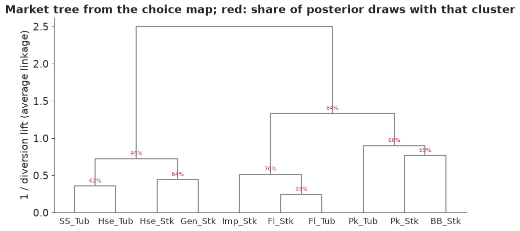
The top split is value versus the rest: house stick and tub, generic and Shedd's form a branch in 95% of posterior draws, and the six national-brand products the other branch in 84%. Within the national brands, the Fleischmann's pair is the most certain cluster of all (93%), with Imperial joining it in 70% of draws; Parkay stick, Blue Bonnet and Parkay tub group together in 66%. The finer splits (which two value products pair first; Parkay stick with Blue Bonnet) are close to coin tosses, and the tree says so. Grouping by form would need a branch for the four tubs.
7.3 · Clout and vulnerability
Market structure is also asymmetric: a price cut by one product may steal a lot from another without the reverse being true. Kamakura & Russell (1989) summarise this with two numbers per product from the cross-price elasticities $\eta_{jk} = \frac{\partial s_j}{\partial p_k} \frac{p_k}{s_j}$: clout $=\sum_{j \ne k} \eta_{jk}$ (how much $k$'s price moves everyone else) and vulnerability $=\sum_{k \ne j} \eta_{jk}$ (how much $j$ is moved by everyone else's prices).
def clout_vulnerability(A, b, prices=p_med):
    Pr = special.softmax(A + b[..., None] * prices, axis=-1)
    s = Pr.mean(1)
    cross = -np.einsum("sh,shj,shk->sjk", b, Pr, Pr) / Pr.shape[1]
    eta = cross * prices[None, None, :] / s[:, :, None]
    idx = np.arange(J)
    eta[:, idx, idx] = 0
    return eta.sum(1), eta.sum(2)


fig, axes = plt.subplots(1, 2, figsize=(13, 5), sharex=True, sharey=True)
for ax, (name, (A, b)) in zip(axes, {"pooled logit": pooled_params(idata_logit),
                                    "choice map": (A2, b2)}.items()):
    clout, vuln = clout_vulnerability(A, b)
    for j, p in enumerate(PRODUCTS):
        colr = BLUE if p.endswith("Stk") else ORANGE
        cx, vy = np.quantile(clout[:, j], [0.05, 0.5, 0.95]), np.quantile(vuln[:, j], [0.05, 0.5, 0.95])
        ax.plot(cx[[0, 2]], [vy[1]] * 2, color=colr, lw=1)
        ax.plot([cx[1]] * 2, vy[[0, 2]], color=colr, lw=1)
        ax.plot(cx[1], vy[1], "o", color=colr)
        ax.annotate(p, (cx[1], vy[1]), xytext=(4, 3), textcoords="offset points", fontsize=8)
    ax.set_xscale("log")
    ax.set_xlabel("clout (sum of cross-elasticities it causes)")
    ax.set_title(name)
axes[0].set_ylabel("vulnerability (sum of cross-elasticities it suffers)");
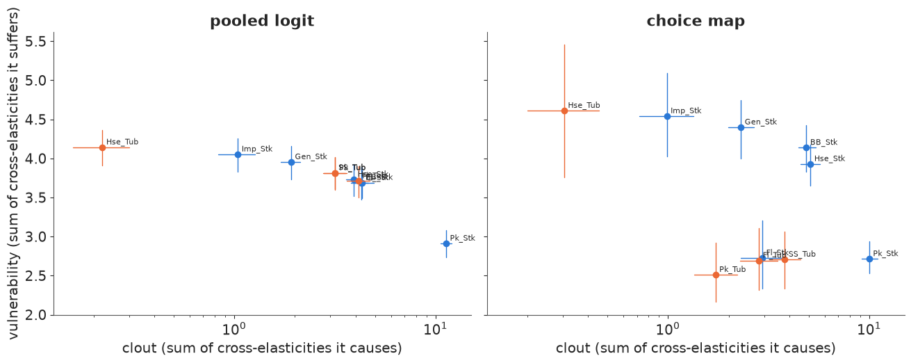
In the pooled logit, vulnerability is nearly the same for every product (3.7-4.1, with the big Parkay stick lower), because cross-elasticities depend only on the other product's share and price. The choice map splits the products into two groups. Low vulnerability: Fleischmann's stick and tub, Parkay tub, Shedd's Spread and Parkay stick - products with a clientele of their own (long arrows on the map) or, for Parkay stick, buyers everywhere. High vulnerability: Blue Bonnet, the house stick, the generic and Imperial, whose buyers also buy the products around them and move when those are on promotion. Parkay stick has by far the most clout in both models. This kind of asymmetry - who steals from whom on promotion - is what Allenby & Rossi (1991) studied in these data.
8 · A merger screen
8.1 · Upward pricing pressure
Suppose brand A buys brand B. Before the merger, when A raised the price of its product $i$, the buyers it lost to B's product $j$ were simply lost. After the merger, they are recaptured, and the margin earned on them offsets the loss - so the merged firm has an incentive to raise $i$'s price. The gross upward pricing pressure index (Farrell & Shapiro 2010; used in the 2010 US Horizontal Merger Guidelines) measures that incentive as a fraction of $i$'s price:
$$\text{GUPPI}_i = \sum_{j \in B} D_{i \to j}\; m_j \,\frac{p_j}{p_i},$$
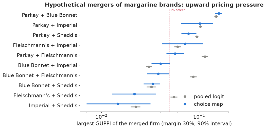
with $m_j$ the percentage margin on $j$. Competition authorities often treat a GUPPI below about 5% as unlikely to cause concern. Everything hinges on the diversion ratios, which is why market structure matters here: the logit says diversion follows size, the map says it follows the submarkets.
Two honest caveats before computing anything. The data contain only margarine purchases, so a household that stops buying margarine is invisible: every diversion ratio is within the category and the ratios sum to one. Real diversion is smaller (some buyers switch to butter or leave), so absolute GUPPIs here are upper bounds, and the ranking of mergers is the robust output. And margins are not in the data: we assume 30% for every product and note how the answer scales with that assumption (GUPPI is proportional to it).
We treat each national brand as a firm (Parkay owns its stick and tub, Fleischmann's likewise) and screen every pair of the five national brands - hypothetical mergers, not a statement about who owned what in the 1980s. The house brand and the generic belong to the retailer and are left out. For a merger we report the largest GUPPI over the two firms' products.
FIRMS = {"Parkay": ["Pk_Stk", "Pk_Tub"], "Blue Bonnet": ["BB_Stk"], "Fleischmann's": ["Fl_Stk", "Fl_Tub"],
         "Imperial": ["Imp_Stk"], "Shedd's": ["SS_Tub"]}
MARGIN = 0.30


def guppi(D, a, b):
    """Max GUPPI over products of firms a and b after they merge: (S,) draws."""
    out = []
    for f, g in [(a, b), (b, a)]:
        for i in FIRMS[f]:
            ii = PRODUCTS.index(i)
            out.append(sum(D[:, PRODUCTS.index(j), ii] * MARGIN * p_med[PRODUCTS.index(j)] / p_med[ii]
                           for j in FIRMS[g]))
    return np.max(out, axis=0)


firm_names = list(FIRMS)
mergers = [(a, b) for n, a in enumerate(firm_names) for b in firm_names[n + 1:]]
res = []
for a, b in mergers:
    for name, D in [("pooled logit", D_logit), ("choice map", D_map)]:
        g = guppi(D, a, b)
        res.append(dict(merger=f"{a} + {b}", model=name, lo=np.quantile(g, 0.05), med=np.median(g),
                        hi=np.quantile(g, 0.95), p_over_5=(g > 0.05).mean()))
res = pd.DataFrame(res)
order = res[res.model == "choice map"].sort_values("med")["merger"].tolist()

fig, ax = plt.subplots(figsize=(9, 5))
for k, (name, colr, off) in enumerate([("pooled logit", GREY, -0.15), ("choice map", BLUE, 0.15)]):
    r = res[res.model == name].set_index("merger").loc[order]
    y = np.arange(len(order)) + off
    ax.hlines(y, r["lo"], r["hi"], color=colr, lw=2.5)
    ax.plot(r["med"], y, "o", color=colr, label=name)
ax.axvline(0.05, color=RED, ls="--", lw=1)
ax.text(0.051, len(order) - 0.6, "5% screen", color=RED, fontsize=8)
ax.set_yticks(range(len(order)), order)
ax.set_xscale("log")
ax.set_xlabel(f"largest GUPPI of the merged firm (margin {MARGIN:.0%}; 90% interval)")
ax.set_title("Hypothetical mergers of margarine brands: upward pricing pressure")
ax.legend(loc="lower right");
tab = res.pivot(index="merger", columns="model", values=["med", "p_over_5"]).loc[order[::-1]]
tab.columns = [f"{m}: {'GUPPI median' if v == 'med' else 'P(GUPPI > 5%)'}" for v, m in tab.columns]
tab.round(3)
| choice map: GUPPI median | pooled logit: GUPPI median | choice map: P(GUPPI > 5%) | pooled logit: P(GUPPI > 5%) | |
|---|---|---|---|---|
| merger | ||||
| Parkay + Blue Bonnet | 0.159 | 0.149 | 1.000 | 1.000 |
| Parkay + Imperial | 0.102 | 0.103 | 0.998 | 1.000 |
| Parkay + Shedd's | 0.078 | 0.095 | 1.000 | 1.000 |
| Fleischmann's + Imperial | 0.072 | 0.060 | 0.878 | 1.000 |
| Parkay + Fleischmann's | 0.056 | 0.114 | 0.802 | 1.000 |
| Blue Bonnet + Imperial | 0.040 | 0.031 | 0.050 | 0.000 |
| Blue Bonnet + Fleischmann's | 0.038 | 0.087 | 0.040 | 1.000 |
| Blue Bonnet + Shedd's | 0.033 | 0.032 | 0.000 | 0.000 |
| Fleischmann's + Shedd's | 0.022 | 0.055 | 0.005 | 0.979 |
| Imperial + Shedd's | 0.015 | 0.022 | 0.000 | 0.000 |
8.2 · What the screen says
The pooled logit flags six of the ten mergers, all with near-certainty, essentially by size: anything with Parkay, plus Blue Bonnet + Fleischmann's and Fleischmann's + Shedd's. Its intervals are narrow because it is confident about a substitution pattern it assumed.
The choice map changes the verdict where the structure says it should:
- Fleischmann's with a brand in another tier is cleared. Blue Bonnet + Fleischmann's falls from
about 9% to 4% (P > 5% only 0.04), Fleischmann's + Shedd's from 5.5% to 2% (P = 0.005), and Parkay
- Fleischmann's from 11% to 6% (P = 0.80). Fleischmann's buyers who face a price rise go to the other Fleischmann's product or to Imperial, not to the mainstream or value brands.
- Fleischmann's + Imperial, the two premium brands, is the merger whose GUPPI goes up (6% to 7%, P = 0.88). It now ranks above Parkay + Fleischmann's, the opposite of the logit's order. Its interval is wide (Imperial has 74 purchases in the panel), and the screen says so.
- Parkay + Blue Bonnet stays the most worrying merger in both models: the two mainstream sticks are each other's closest substitutes and big.
A Bayesian screen reports the probability that a merger crosses the threshold, not just a point estimate, and that is what a case team needs to decide which mergers deserve a closer look. The absolute numbers are inflated by the missing outside good and scale with the assumed margin; the re-ranking driven by the structure is the robust part.
Summary
- Market structure is substitution: where the buyers of a product go when it gets dearer. The switching matrix hints at it but mixes heterogeneity, prices and state dependence, and its small cells are noisy. In the margarine panel it showed premium, value and mainstream blocks, not sticks vs tubs.
- The pooled logit has no market structure by construction: diversion is proportional to share (lift exactly 1), and elasticities are proportional to price, which made the expensive tubs the most price-sensitive products.
- Nested-logit tests of competing hierarchies were nearly powerless: form and tier nests both got $\lambda \approx 0.7$, but no nesting improved held-out purchases by more than about two standard errors, and pooled nesting cannot tell substitution from "bought by the same households".
- A factor-structured hierarchical logit (a choice map) improved held-out purchases by about 250 nats. Its loadings had r_hat near 2 with no sampling problem at all - the map is identified only up to rotation - while $\Lambda\Lambda^\top$, probabilities and diversion ratios converged. Procrustes alignment of the draws gives a drawable map with honest uncertainty.
- Apparent loyalty was mostly heterogeneity: the last-purchase effect fell from odds x6 (pooled) to x1.4 once households had their own tastes.
- Simulated purchase histories reproduced the repeat rate and the blocks of the switching matrix, and came much closer to the spread of households over products; the pooled logit matched only the repeat rate.
- The market is organised by tier, not form: value (house, generic, Shedd's) versus national brands, and within those a Fleischmann's-plus-Imperial premium group. Fleischmann's is the only brand whose buyers cross forms; Parkay's do not.
- Merger screen: the share-driven logit flagged six of ten hypothetical mergers; the choice map cleared Fleischmann's mergers with other-tier brands and raised the premium-brand merger above Parkay + Fleischmann's. Within-category diversion and an assumed margin make absolute GUPPIs upper bounds; the re-ranking is the robust output.
Try it yourself
- Demographics on the map.
data.load("margarine_demos")has income, family size, education and retirement for every household. Let $\mathbf{z}_h$'s mean depend on them ($\mathbf{z}_h \sim N(\Gamma \mathbf{w}_h, I)$) - which demographic moves households toward the premium arrows? Does it improve held-out purchases, or only explain the map? - An outside good. Diversion ratios here sum to one because non-purchase is unobserved. Add a "no purchase" option with an assumed trip-level purchase probability (say 1 in 4 trips includes margarine) and recompute the GUPPIs. How much do they shrink, and does the ranking survive?
- Ideal points instead of vectors. Replace $\boldsymbol{\lambda}_j^\top \mathbf{z}_h$ by $-\lVert \mathbf{z}_h - \mathbf{x}_j \rVert^2$ (an ideal-point map: households like products near them). Is it identified up to rotation and translation? Does it predict held-out purchases better, and does the market tree change?