A marketing-mix model (MMM) has to say what one more pound of spend buys, and that depends on the shape of the response curve: does each extra pound buy a bit less (concave), a bit more (convex), or does the curve start slowly, then climb, then flatten (S-shaped)? Every MMM package chooses a family for you:
| library / tradition | default response curve | shapes it can take |
|---|---|---|
| Robyn (Meta), Meridian (Google), E33 here | Hill $x^n / (K^n + x^n)$ | concave or S |
| PyMC-Marketing | logistic saturation $(1 - e^{-\lambda x}) / (1 + e^{-\lambda x})$ | concave only |
| econometrics | power $x^k$, or $\log(1 + x)$ | concave or convex, never saturates |
A family is a prior with zero probability outside it. If the truth is S-shaped and the family is concave-only, no amount of data can find the S. This notebook builds one smooth family that contains all three behaviours, as a custom JAX function, and puts it in a Bayesian MMM so that the posterior, not the software default, chooses the shape. We also find out where the data cannot choose.
The plan: the family and its geometry (sections 1-2); a numerically safe JAX implementation with tests (3); how closely it reproduces the standard curves, and how to carry a prior over from one of them (4-5); the PyMC model and a fake-data check (6-7); a real brand (8); performance (9).
import logging
import time
import warnings

import arviz as az
import jax
import jax.numpy as jnp
import matplotlib.pyplot as plt
import numpy as np
import optax
import pandas as pd
import pymc as pm
import pytensor
import pytensor.tensor as pt
from IPython.display import display
from matplotlib.colors import ListedColormap
from matplotlib.ticker import FixedLocator, NullLocator

from pymc_challenges import data

jax.config.update("jax_enable_x64", True)
RANDOM_SEED = 45
rng = np.random.default_rng(RANDOM_SEED)
az.style.use("arviz-variat")
logging.getLogger("pymc").setLevel(logging.WARNING)  # several fits: no sampler banner per fit
# Expected and harmless: Numba runs the JAX node in object mode (section 9 measures the cost)
warnings.filterwarnings("ignore", message="Numba will use object mode")
warnings.filterwarnings("ignore", message="Skipping Check")  # JAX drops PyMC's parameter checks
BLUE, ORANGE, AQUA, GREY, PURPLE, RED = "#2a78d6", "#eb6834", "#1baf7a", "#8a8a86", "#8c5ac8", "#c8384e"
print(f"PyMC {pm.__version__}, ArviZ {az.__version__}, PyTensor {pytensor.__version__}, "
      f"JAX {jax.__version__}, optax {optax.__version__}")
PyMC 6.3.2, ArviZ 1.3.0, PyTensor 3.3.2, JAX 0.11.2, optax 0.2.8
1 · Six standard curves, six different answers
Below are six textbook response curves. Each is scaled to pass through the same point: at the reference spend $x = 1$ (think "an average week") the channel brings in one unit of response. They agree there by construction, and they disagree about everything a budget decision needs: the slope at $x = 1$ (the marginal return), what happens at half the spend, and what happens at twice the spend.
X_PLOT = np.linspace(0, 3, 301)


def hill_np(x, K, n):
    return x**n / (K**n + x**n)


def logistic_np(x, lam):
    return (1 - np.exp(-lam * x)) / (1 + np.exp(-lam * x))


standard = {
    "Hill, S-shaped (K=1.2, n=3)": lambda x: hill_np(x, 1.2, 3.0),
    "Hill, concave (K=1, n=1)": lambda x: hill_np(x, 1.0, 1.0),
    "logistic saturation (λ=1)": lambda x: logistic_np(x, 1.0),
    "power, concave (x^0.5)": lambda x: np.sqrt(x),
    "power, convex (x^1.5)": lambda x: x**1.5,
    "log(1 + 2x)": lambda x: np.log1p(2 * x),
}
fig, axes = plt.subplots(1, 2, figsize=(12, 4.2))
colors = [BLUE, ORANGE, AQUA, PURPLE, RED, GREY]
slopes = {}
for (name, f), col in zip(standard.items(), colors):
    y_ = f(X_PLOT) / f(1.0)
    axes[0].plot(X_PLOT, y_, color=col, lw=2, label=name)
    slopes[name] = (f(1.001) - f(0.999)) / 0.002 / f(1.0)
axes[0].axvline(1, color=GREY, lw=0.8, ls=":")
axes[0].set(xlabel="spend (1 = reference week)", ylabel="response (1 at the reference)",
            title="Same response at the reference spend...", ylim=(0, 3.2))
axes[0].legend(fontsize=8)
names = list(slopes)
axes[1].barh(names, [slopes[n] for n in names], color=colors)
axes[1].axvline(1, color=GREY, lw=0.8, ls=":")
axes[1].invert_yaxis()
axes[1].set(xlabel="marginal return at the reference (1 = the average return)",
            title="...but marginal returns that differ by a factor of 4")
[Text(0.5, 0, 'marginal return at the reference (1 = the average return)'),
 Text(0.5, 1.0, '...but marginal returns that differ by a factor of 4')]
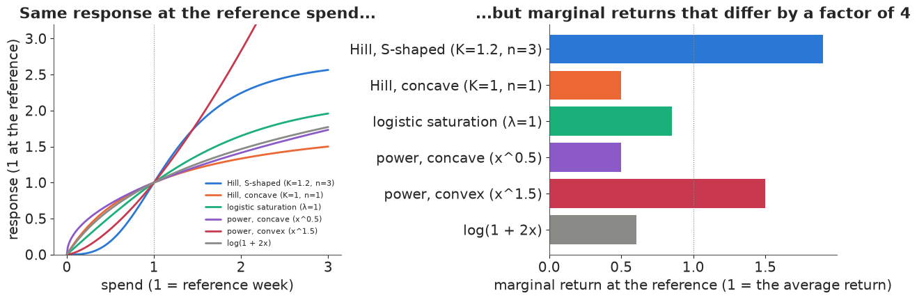
The marginal return at the reference spend, relative to the average return, ranges from 0.5 (the concave Hill and square-root curves) to 1.9 (the S-curve, which is at its steepest near the reference). "Spend 10% more" is a good or a bad idea depending on which curve you assumed.
2 · The Weibull response family
The Weibull distribution's CDF, $1 - \exp(-(x/\lambda)^k)$, has long been used as a growth and dose-response curve, and Robyn uses Weibull CDF/PDF shapes for adstock. Here we use it as the saturation curve and write it in a form that keeps the power-law limit inside the family:
$$ f(x;\, k, c) \;=\; \frac{1 - e^{-c\,x^k}}{1 - e^{-c}}, \qquad k > 0,\; c \ge 0, \qquad\text{so that } f(1) = 1 . $$
The response of a channel is $\beta\, f(x)$, where $x$ is (adstocked) spend divided by its average and $\beta$ is the response in an average week. The normalisation at $x = 1$ is what makes $\beta$ interpretable and separates "how big" ($\beta$) from "what shape" ($k$, $c$).
Three behaviours, one family.
- Power curves as $c \to 0$. Since $1 - e^{-u} \approx u$ for small $u$, the ratio tends to $c x^k / c = x^k$: the econometrician's power curve, concave for $k < 1$, linear at $k = 1$, convex for $k > 1$, never saturating. The limit is smooth: $c$ is a continuous "how much saturation" knob that is exactly zero for a power curve.
- Concave saturation for $k \le 1$, $c > 0$. At $k = 1$ it is the exponential saturation curve $1 - e^{-cx}$ (the numerator of the logistic saturation curve); for $k < 1$ it rises even faster at first.
- S-curves for $k > 1$, $c > 0$. The second derivative has the sign of $(k - 1) - c k x^k$, so there is exactly one inflection point
$$ x^\ast = \left(\frac{k - 1}{c\,k}\right)^{1/k}. $$
Below $x^\ast$ each extra pound buys more than the last; above it, less. Whether a fitted curve "is" S-shaped therefore depends on whether $x^\ast$ lies inside the range of spend you have seen. If $x^\ast$ is far to the right, the curve is convex over the whole data; if it is near zero, the curve is concave over the whole data. The shape map below colours the $(k, c)$ plane by what the curve looks like on $0 \le x \le 2.5$, the range this notebook's brand actually spends in.
X_RANGE = 2.5  # the spend range we care about, in units of an average week


def weibull_np(x, k, c):
    """Reference NumPy version, for plotting only (section 3 writes the careful one)."""
    c = np.maximum(c, 1e-12)
    return -np.expm1(-c * x**k) / -np.expm1(-c)


def inflection(k, c):
    """x* = ((k - 1) / (c k))^(1/k) for k > 1; inf where there is none."""
    with np.errstate(invalid="ignore", divide="ignore", over="ignore"):
        return np.where(k > 1, ((k - 1) / np.maximum(c * k, 1e-300)) ** (1 / k), np.inf)


def shape_class(k, c, x_max=X_RANGE, tol=0.03):
    """0 concave, 1 ~linear, 2 convex, 3 S-shaped (inflection inside (0, x_max))."""
    k, c = np.broadcast_arrays(np.asarray(k, float), np.asarray(c, float))
    xs = np.linspace(0, x_max, 101)
    curves = weibull_np(xs[:, None], k.ravel()[None], c.ravel()[None])  # (x, points)
    near_linear = (np.abs(curves - xs[:, None]).max(0) < tol * x_max).reshape(k.shape)
    x_star = inflection(k, c)
    out = np.where(k <= 1, 0, np.where(x_star < x_max, 3, 2))
    return np.where(near_linear, 1, out)


SHAPE_NAMES = ["concave", "≈ linear", "convex", "S-shaped"]
SHAPE_CMAP = ListedColormap(["#cfe0f5", "#e6e6e3", "#f7d5c6", "#d5ecdf"])
kg = np.exp(np.linspace(np.log(0.3), np.log(5), 240))
cg = np.exp(np.linspace(np.log(1e-3), np.log(20), 240))
KG, CG = np.meshgrid(kg, cg, indexing="xy")
SHAPE_GRID = shape_class(KG, CG)


def draw_shape_map(ax, labels=True):
    ax.pcolormesh(kg, cg, SHAPE_GRID, cmap=SHAPE_CMAP, vmin=-0.5, vmax=3.5, shading="auto",
                  rasterized=True)
    ax.set(xscale="log", yscale="log", xlabel="shape k", ylabel="saturation c")
    ax.xaxis.set_major_locator(FixedLocator([0.3, 0.5, 1, 2, 3, 5]))
    ax.xaxis.set_minor_locator(NullLocator())
    ax.set_xticklabels(["0.3", "0.5", "1", "2", "3", "5"])
    if labels:
        for (kx, cy), name in zip([(0.45, 0.3), (1.0, 0.0022), (3.2, 0.0025), (3.0, 2.0)], SHAPE_NAMES):
            ax.text(kx, cy, name, ha="center", fontsize=10, color="#333333", weight="bold")


examples = {"A": (0.5, 0.002), "B": (0.6, 1.5), "C": (1.0, 0.8), "D": (1.8, 0.005),
            "E": (2.5, 0.4), "F": (3.5, 3.0)}
fig, axes = plt.subplots(1, 2, figsize=(12, 4.8), gridspec_kw={"width_ratios": [1.1, 1]})
draw_shape_map(axes[0])
for lab, (k_, c_) in examples.items():
    axes[0].plot(k_, c_, "o", color="k", ms=5)
    axes[0].annotate(lab, (k_, c_), xytext=(4, 4), textcoords="offset points", weight="bold")
axes[0].set_title(f"The shape map: what the curve looks like on 0 ≤ x ≤ {X_RANGE}")
for (lab, (k_, c_)), col in zip(examples.items(), [PURPLE, BLUE, AQUA, RED, ORANGE, GREY]):
    cls = SHAPE_NAMES[int(shape_class(k_, c_))]
    axes[1].plot(X_PLOT, weibull_np(X_PLOT, k_, c_), color=col, lw=2,
                 label=f"{lab}: k={k_}, c={c_} ({cls})")
axes[1].axvspan(X_RANGE, 3, color=GREY, alpha=0.12)
axes[1].set(xlabel="spend x", ylabel="f(x)", ylim=(0, 3.2), title="Curves at the marked points")
axes[1].legend(fontsize=8)
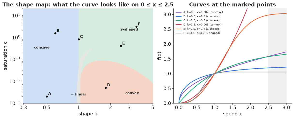
Points A and D are power curves (tiny $c$); B and C saturate; E and F are S-curves whose inflection points (about 1.2 and 0.7) lie inside the data range. The boundaries of the map are where a decision changes character: crossing from "convex" to "S-shaped" means an inflection point has entered the data. Nothing about the family is discontinuous there, which is exactly what NUTS needs.
3 · A custom JAX function that does not break
The formula is one line. Written naively, it breaks in three places that a sampler will visit:
def weibull_naive(x, k, c):
    return (1 - jnp.exp(-c * x**k)) / (1 - jnp.exp(-c))


xs = jnp.array([0.5, 1.0, 2.0])
print("1. c = 0 exactly (a pure power curve):", weibull_naive(xs, 1.5, 0.0))
for c_small in (1e-6, 1e-10, 1e-13):
    rel = np.max(np.abs(weibull_naive(xs, 1.5, c_small) / xs**1.5 - 1))
    print(f"2. c = {c_small:.0e}: relative error vs the exact limit x^k = {rel:.1e}")
with jax.enable_x64(False):
    x32 = jnp.array([0.5, 1.0, 2.0], dtype=jnp.float32)
    for c_small in (1e-4, 1e-6):
        rel32 = np.max(np.abs(weibull_naive(x32, 1.5, jnp.float32(c_small)) / x32**1.5 - 1))
        print(f"   float32, c = {c_small:.0e}: relative error {rel32:.1e}")
pow_via_log = lambda x, k: jnp.where(x > 0, jnp.exp(k * jnp.log(x)), 0.0)  # noqa: E731
print("3. d/dk of x^k at x = 0, written as exp(k log x) under a where:",
      jax.grad(pow_via_log, argnums=1)(0.0, 1.5))
print("   d/dx of x^0.5 at x = 0 with jnp.power:", jax.grad(lambda x: x**0.5)(0.0))
1. c = 0 exactly (a pure power curve): [nan nan nan]
2. c = 1e-06: relative error vs the exact limit x^k = 9.1e-07
2. c = 1e-10: relative error vs the exact limit x^k = 1.2e-06
2. c = 1e-13: relative error vs the exact limit x^k = 1.7e-03
   float32, c = 1e-04: relative error 4.4e-04
   float32, c = 1e-06: relative error 2.3e-02
3. d/dk of x^k at x = 0, written as exp(k log x) under a where: nan
   d/dx of x^0.5 at x = 0 with jnp.power: inf
- $c = 0$ is $0/0$. It is a legitimate parameter value (the power curve), and a prior on $c$ that allows it will sample close to it.
- Small $c$ cancels catastrophically. $1 - e^{-u}$ for tiny $u$ subtracts two nearly equal numbers, and the relative error grows like (machine precision) / $c$. In float64 it is $10^{-6}$ at $c = 10^{-10}$ and $10^{-3}$ at $c = 10^{-13}$; in float32 (JAX's default, and what a GPU prefers) the same happens about eight orders of magnitude sooner: a 2% error at $c = 10^{-6}$.
- Zero spend. Weeks with no spend give $x = 0$. The derivative of $x^k$ with respect to
$x$ is infinite there for $k < 1$, and the common idiom
where(x > 0, exp(k log x), 0)gives a NaN gradient even though its value is fine:wheredifferentiates both branches and multiplies the untaken one by zero, and $0 \times (-\infty) = $ NaN. (PyTensor'sswitchdoes the same; see the gotcha from E08.)
The fixes are standard:
- write $\frac{1 - e^{-cz}}{c} = z \cdot \phi(cz)$ with $\phi(u) = (1 - e^{-u})/u$, evaluated
with
expm1and replaced by its Taylor series $1 - u/2 + u^2/6 - u^3/24$ below $u = 10^{-4}$ (where the truncation error, about $u^4/120$, is below float64 rounding). Then $f(x) = x^k\,\phi(c x^k) / \phi(c)$, and $c = 0$ is an ordinary point. - the double-
wheretrick: first replace the bad input by a harmless one, then compute, then select. The untaken branch is now finite, so its zero weight gives a zero gradient.
SERIES_BELOW = 1e-4


def phi(u):
    """(1 - exp(-u)) / u for u >= 0, with phi(0) = 1; stable at all u, including under grad."""
    small = u < SERIES_BELOW
    u_safe = jnp.where(small, 1.0, u)  # double-where: the untaken branch never sees u = 0
    return jnp.where(small, 1 - u / 2 + u**2 / 6 - u**3 / 24, -jnp.expm1(-u_safe) / u_safe)


def safe_pow(x, k):
    """x**k for x >= 0 with finite gradients in x and k at x = 0 (value and gradients 0 there)."""
    pos = x > 0
    x_safe = jnp.where(pos, x, 1.0)
    return jnp.where(pos, jnp.exp(k * jnp.log(x_safe)), 0.0)


def weibull(x, k, c):
    """Weibull response f(x) = (1 - exp(-c x^k)) / (1 - exp(-c)), exact at c = 0 (f = x^k)."""
    z = safe_pow(x, k)
    return z * phi(c * z) / phi(c)


def geometric_adstock(x, theta):
    """x (week, channel), theta (channel,) -> a_t = theta a_{t-1} + (1 - theta) x_t.

    The (1 - theta) weight keeps the long-run level of a constant spend unchanged, so x = 1 still
    means "an average week". The recursion starts from the mean of the first 8 weeks."""
    def step(a, x_t):
        a = theta * a + (1 - theta) * x_t
        return a, a

    _, out = jax.lax.scan(step, x[:8].mean(axis=0), x)
    return out


def media_transform(x, theta, k, c):
    """Spend (week, channel) -> adstocked, saturated response curves (week, channel)."""
    return weibull(geometric_adstock(x, theta), k, c)


weibull_jit = jax.jit(weibull)
print("c = 0 now gives x^k:          ", weibull_jit(xs, 1.5, 0.0), "vs", xs**1.5)
print("d/dk at x = 0:                ", jax.grad(weibull, argnums=1)(0.0, 1.5, 0.5))
print("d/dx at x = 0, k = 0.5:       ", jax.grad(weibull, argnums=0)(0.0, 0.5, 0.5))
c = 0 now gives x^k: [0.35355339 1. 2.82842712] vs [0.35355339 1. 2.82842712]
d/dk at x = 0:                 0.0
d/dx at x = 0, k = 0.5:        0.0
Tests
A likelihood component is code, so it gets unit tests. Four properties:
- the $c \to 0$ limit is the power curve, and the function is continuous across the series switch at $c x^k = 10^{-4}$;
- gradients in $k$ and $c$ agree with central finite differences, on both sides of the switch;
- float32 agrees with float64 to float32 precision (so it would run on a GPU);
- the second derivative from
jax.grad(jax.grad(...))changes sign exactly at the closed-form inflection point $x^\ast$.
# 1. limit and continuity
for c_ in (1e-2, 1e-4, 1e-8, 0.0):
    err = float(jnp.max(jnp.abs(weibull(xs, 1.5, c_) - xs**1.5)))
    print(f"c = {c_:.0e}: max |f - x^k| = {err:.1e}")
u_edge = SERIES_BELOW
jump = abs(float(phi(u_edge * (1 - 1e-12)) - phi(u_edge * (1 + 1e-12))))
print(f"jump in phi across the series switch: {jump:.1e}")

# 2. gradients vs finite differences, both sides of the switch
test_points = [(0.7, 1.3, 0.0), (0.7, 1.3, 0.99e-4), (0.7, 1.3, 1.01e-4), (1.8, 0.6, 2.0),
               (2.4, 3.5, 5.0), (0.0, 0.8, 1.0)]
worst = 0.0
for x_, k_, c_ in test_points:
    g = jax.grad(weibull, argnums=(1, 2))(x_, k_, c_)
    h = 1e-6
    fd_k = (weibull(x_, k_ + h, c_) - weibull(x_, k_ - h, c_)) / (2 * h)
    fd_c = (weibull(x_, k_, c_ + h) - weibull(x_, k_, max(c_ - h, 0.0))) / (h + min(h, c_))
    worst = max(worst, abs(float(g[0] - fd_k)), abs(float(g[1] - fd_c)))
print(f"worst |autodiff - finite difference| over {len(test_points)} points: {worst:.1e}")

# 3. float32 vs float64
xg64 = jnp.linspace(0, 3, 50)
with jax.enable_x64(False):
    f32 = np.asarray(weibull(jnp.asarray(xg64, jnp.float32), jnp.float32(2.2), jnp.float32(3e-5)))
f64 = np.asarray(weibull(xg64, 2.2, 3e-5))
print(f"float32 vs float64, c = 3e-5: max relative difference {np.max(np.abs(f32[1:] / f64[1:] - 1)):.1e}")

# 4. inflection point
k_, c_ = 2.5, 0.4
d2 = jax.vmap(jax.grad(jax.grad(weibull)), in_axes=(0, None, None))
xfine = jnp.linspace(0.05, 3, 20001)
x_sign_change = float(xfine[jnp.argmax(d2(xfine, k_, c_) < 0)])
print(f"inflection: second derivative changes sign at x = {x_sign_change:.4f}, "
      f"closed form x* = {((k_ - 1) / (c_ * k_)) ** (1 / k_):.4f}")
c = 1e-02: max |f - x^k| = 2.6e-02
c = 1e-04: max |f - x^k| = 2.6e-04
c = 1e-08: max |f - x^k| = 2.6e-08
c = 0e+00: max |f - x^k| = 4.4e-16
jump in phi across the series switch: 1.1e-16
worst |autodiff - finite difference| over 6 points: 4.9e-09
float32 vs float64, c = 3e-5: max relative difference 2.9e-07
inflection: second derivative changes sign at x = 1.1762, closed form x* = 1.1761
All four pass: the error against $x^k$ falls in proportion to $c$ and is exactly zero at $c = 0$, the switch is seamless, gradients agree with finite differences to about $10^{-9}$ (the finite-difference error itself), float32 is good to about $10^{-7}$, and autodiff locates the inflection point where the algebra says it is.
4 · How well does one family imitate the others?
If the Weibull family is to stand in for the standard transforms, it has to reproduce them
closely over the range of the data. That is a curve-fitting question with thousands of
independent fits, which is what jax.vmap is for: write one least-squares fit (Adam from
optax, 3,000 steps in a lax.scan, three starting points), then map it over a whole grid of
target curves. The free parameters are $(\log\beta, \log k, \log c)$; the error is the largest
gap between the curves on $0 \le x \le 3$, as a fraction of the target's maximum.
X_FIT = jnp.linspace(0, 3, 121)
STARTS = jnp.array([[0.0, 0.0, -1.0], [0.0, 0.7, 0.0], [0.0, -0.5, 1.0]])
adam = optax.adam(0.05)


def weibull_curve(p, x=X_FIT):
    return jnp.exp(p[0]) * weibull(x, jnp.exp(p[1]), jnp.exp(p[2]))


def fit_from(target, p0, steps=3000):
    loss = lambda p: jnp.mean((weibull_curve(p) - target) ** 2)  # noqa: E731

    def step(carry, _):
        p, state = carry
        updates, state = adam.update(jax.grad(loss)(p), state, p)
        return (optax.apply_updates(p, updates), state), None

    (p, _), _ = jax.lax.scan(step, (p0, adam.init(p0)), None, length=steps)
    return p, jnp.max(jnp.abs(weibull_curve(p) - target)) / jnp.max(target)


def fit_best(target):
    ps, errs = jax.vmap(fit_from, in_axes=(None, 0))(target, STARTS)
    best = jnp.argmin(errs)
    return ps[best], errs[best]


fit_many = jax.jit(jax.vmap(fit_best))  # (n_curves, 121) -> params (n_curves, 3), errors (n_curves,)

K_GRID = np.linspace(0.3, 3.0, 28)
N_GRID = np.linspace(0.5, 4.0, 29)
KK, NN = np.meshgrid(K_GRID, N_GRID, indexing="ij")
hill_targets = jnp.asarray(hill_np(np.asarray(X_FIT)[None], KK.ravel()[:, None], NN.ravel()[:, None]))
t0 = time.perf_counter()
hill_params, hill_err = jax.block_until_ready(fit_many(hill_targets))
print(f"{len(hill_targets)} Hill curves x 3 starts x 3000 Adam steps: {time.perf_counter() - t0:.1f} s")
HILL_ERR = np.asarray(hill_err).reshape(KK.shape)
print(f"max error over the Hill grid: median {100 * np.median(HILL_ERR):.1f}%, "
      f"90th percentile {100 * np.quantile(HILL_ERR, 0.9):.1f}%, worst {100 * HILL_ERR.max():.1f}%")
812 Hill curves x 3 starts x 3000 Adam steps: 4.1 s
max error over the Hill grid: median 1.2%, 90th percentile 3.6%, worst 4.7%
gallery = {
    "logistic saturation λ=1": logistic_np(X_FIT, 1.0),
    "logistic saturation λ=3": logistic_np(X_FIT, 3.0),
    "Michaelis-Menten x/(0.8+x)": X_FIT / (0.8 + X_FIT),
    "tanh(x/1.5)": np.tanh(X_FIT / 1.5),
    "log(1 + 2x)": np.log1p(2 * X_FIT),
    "power x^0.5": np.sqrt(X_FIT),
    "power x^1.6": X_FIT**1.6,
    "shifted sigmoid": 1 / (1 + np.exp(-3 * (X_FIT - 1.5))) - 1 / (1 + np.exp(4.5)),
}
gal_params, gal_err = fit_many(jnp.asarray(np.stack([np.asarray(v) for v in gallery.values()])))
gal_params, gal_err = np.asarray(gal_params), np.asarray(gal_err)
display(pd.DataFrame({"k": np.exp(gal_params[:, 1]), "c": np.exp(gal_params[:, 2]),
                      "max error (% of max)": 100 * gal_err}, index=list(gallery)).round(3))
| k | c | max error (% of max) | |
|---|---|---|---|
| logistic saturation λ=1 | 1.143 | 0.594 | 0.742 |
| logistic saturation λ=3 | 1.191 | 2.323 | 1.147 |
| Michaelis-Menten x/(0.8+x) | 0.839 | 1.080 | 1.449 |
| tanh(x/1.5) | 1.168 | 0.863 | 0.933 |
| log(1 + 2x) | 0.829 | 0.541 | 1.060 |
| power x^0.5 | 0.513 | 0.047 | 0.259 |
| power x^1.6 | 1.643 | 0.017 | 0.387 |
| shifted sigmoid | 3.140 | 0.196 | 1.530 |
fig = plt.figure(figsize=(13, 7.5), layout="constrained")
gs = fig.add_gridspec(2, 5, height_ratios=[1, 1])
ax_h = fig.add_subplot(gs[:, :2])
im = ax_h.pcolormesh(K_GRID, N_GRID, 100 * HILL_ERR.T, cmap="viridis", shading="auto")
fig.colorbar(im, ax=ax_h, label="worst gap on 0 ≤ x ≤ 3 (% of curve max)")
ax_h.set(xlabel="Hill half-saturation K", ylabel="Hill shape n",
         title="Weibull fit to 812 Hill curves")
SHOW = ["logistic saturation λ=1", "Michaelis-Menten x/(0.8+x)", "log(1 + 2x)",
        "power x^0.5", "power x^1.6", "shifted sigmoid"]
gal_names = list(gallery)
gal_axes = [fig.add_subplot(gs[r, 2 + col]) for r in range(2) for col in range(3)]
for ax, name in zip(gal_axes, SHOW):
    i = gal_names.index(name)
    ax.plot(X_FIT, gallery[name], color=GREY, lw=4, alpha=0.6, label="target")
    ax.plot(X_FIT, weibull_curve(jnp.asarray(gal_params[i])), color=BLUE, lw=1.5, label="Weibull fit")
    ax.set_title(f"{name}\n{100 * gal_err[i]:.1f}% max gap", fontsize=9)
    ax.tick_params(labelsize=7)
gal_axes[0].legend(fontsize=7)
fig.suptitle("The Weibull family reproduces standard response curves to within a few percent");
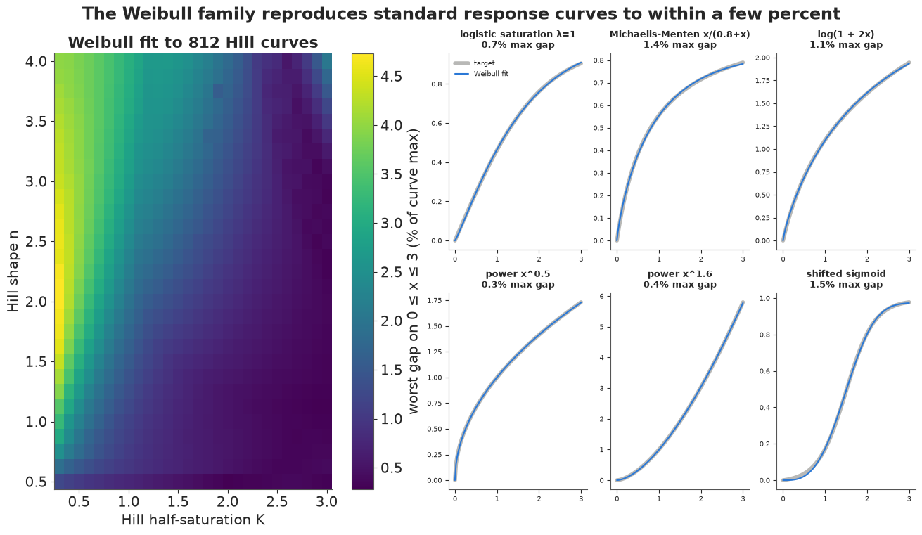
Over the fitted range the family is a very good imitator. Across 812 Hill curves the worst gap is a few percent of the curve's height and usually about 1%; the other standard shapes are reproduced to within about 1.5%. Weekly MMM data are far noisier than that (section 8 finds weekly new customers scattering by about 16% around the model mean), so inside the data no experiment could tell a Hill curve from its Weibull twin. The fits are hardest for Hill curves with large $n$ and large $K$: steep S-curves that are still rising at the edge of the range.
Where the imitation fails: outside the range. Hill curves approach their ceiling like a power of $1/x$; Weibull curves approach theirs exponentially fast. Fitted on $[0, 3]$, the two agree there and part company beyond it:
X_FAR = jnp.linspace(0, 12, 400)
fig, axes = plt.subplots(1, 3, figsize=(13, 3.6), sharey=False)
for ax, (K_, n_) in zip(axes, [(1.0, 1.0), (1.2, 3.0), (2.5, 2.0)]):
    target = hill_np(np.asarray(X_FIT), K_, n_)
    p, e = fit_best(jnp.asarray(target))
    ax.plot(X_FAR, hill_np(np.asarray(X_FAR), K_, n_), color=GREY, lw=4, alpha=0.6, label="Hill")
    ax.plot(X_FAR, weibull_curve(p, X_FAR), color=BLUE, lw=1.5, label="Weibull fitted on [0, 3]")
    ax.axvspan(3, 12, color=ORANGE, alpha=0.08)
    ax.text(7.5, 0.05, "extrapolation", color=ORANGE, ha="center")
    ax.set(title=f"Hill K={K_}, n={n_}", xlabel="spend x")
axes[0].legend(fontsize=8)
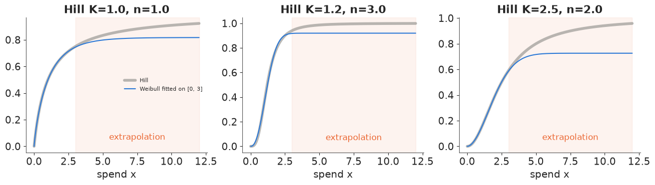
This is not a defect of either family: it shows that the shape of a response curve beyond the data is set by the family, not by the data. Every MMM that recommends quadrupling a budget is reporting its functional form. We come back to this in section 8.
5 · Carrying a Hill prior into the Weibull family
Teams often have priors written for a particular curve: Meridian and Robyn users think in Hill $(K, n)$, and E33 put a prior on the half-saturation point. The same batched fitter translates such a prior: draw curves from the Hill prior, fit each with the Weibull family, and look at the cloud of $(k, c)$ values. Here the prior is $K \sim \text{LogNormal}(\log 1.5, 0.5)$, $n \sim \text{LogNormal}(\log 1.5, 0.4)$, with curves normalised at $x = 1$ and fitted on the data range $[0, 2.5]$.
N_PRIOR = 1000
K_prior = np.exp(rng.normal(np.log(1.5), 0.5, N_PRIOR))
n_prior = np.exp(rng.normal(np.log(1.5), 0.4, N_PRIOR))
X_DATA_RANGE = jnp.linspace(0, X_RANGE, 101)
prior_targets = hill_np(np.asarray(X_DATA_RANGE)[None], K_prior[:, None], n_prior[:, None])
prior_targets /= hill_np(1.0, K_prior, n_prior)[:, None]


def fit_best_range(target):
    """As fit_best, on the data range [0, 2.5]."""
    def fit_from_r(p0):
        loss = lambda p: jnp.mean((weibull_curve(p, X_DATA_RANGE) - target) ** 2)  # noqa: E731

        def step(carry, _):
            p, state = carry
            updates, state = adam.update(jax.grad(loss)(p), state, p)
            return (optax.apply_updates(p, updates), state), None

        (p, _), _ = jax.lax.scan(step, (p0, adam.init(p0)), None, length=3000)
        return p, jnp.max(jnp.abs(weibull_curve(p, X_DATA_RANGE) - target)) / jnp.max(target)

    ps, errs = jax.vmap(fit_from_r)(STARTS)
    return ps[jnp.argmin(errs)], jnp.min(errs)


prior_params, prior_err = jax.jit(jax.vmap(fit_best_range))(jnp.asarray(prior_targets))
log_kc = np.asarray(prior_params)[:, 1:]  # (log k, log c)
print(f"translation error: median {100 * np.median(prior_err):.1f}%, worst {100 * np.max(prior_err):.1f}%")
mean_kc, cov_kc = log_kc.mean(0), np.cov(log_kc.T)
print("translated prior: (log k, log c) ~ MvNormal(mean =", mean_kc.round(2), ", sd =",
      np.sqrt(np.diag(cov_kc)).round(2), ", corr =", round(cov_kc[0, 1] / np.sqrt(np.prod(np.diag(cov_kc))), 2), ")")
translation error: median 0.7%, worst 4.1%
translated prior: (log k, log c) ~ MvNormal(mean = [ 0.28 -0.58] , sd = [0.38 0.75] , corr = -0.58 )
fig, axes = plt.subplots(1, 2, figsize=(12, 4.4))
draw_shape_map(axes[0])
axes[0].scatter(np.exp(log_kc[:, 0]), np.exp(log_kc[:, 1]), s=4, color="k", alpha=0.35)
axes[0].set_title("A Hill prior, translated into (k, c)")
kc_draws = np.exp(rng.multivariate_normal(mean_kc, cov_kc, 200))
for i in range(60):
    axes[1].plot(X_DATA_RANGE, prior_targets[i], color=GREY, lw=0.6, alpha=0.5)
    axes[1].plot(X_DATA_RANGE, weibull_np(np.asarray(X_DATA_RANGE), *kc_draws[i]), color=BLUE,
                 lw=0.6, alpha=0.5)
axes[1].plot([], [], color=GREY, label="Hill prior draws")
axes[1].plot([], [], color=BLUE, label="draws from the translated Weibull prior")
axes[1].set(xlabel="spend x", ylabel="f(x)", ylim=(0, 4), title="Prior curves: before and after")
axes[1].legend(fontsize=8)
print("shape classes, Hill prior draws:", dict(zip(SHAPE_NAMES, np.bincount(
    shape_class(np.exp(log_kc[:, 0]), np.exp(log_kc[:, 1])), minlength=4) / N_PRIOR)))
shape classes, Hill prior draws: {'concave': np.float64(0.225), '≈ linear': np.float64(0.003), 'convex': np.float64(0.015), 'S-shaped': np.float64(0.757)}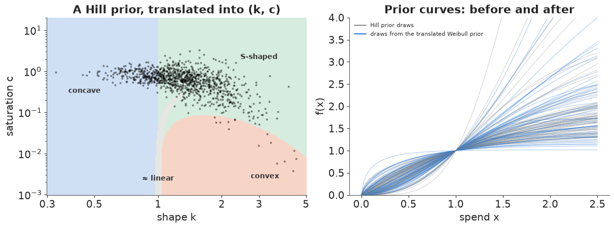
The Hill prior becomes a tilted cloud, mostly in the S-shaped region with a tail into the concave one, and $\log k$ and $\log c$ are negatively correlated: a steeper rise (larger $k$) goes with a later onset of saturation (smaller $c$). A bivariate normal on $(\log k, \log c)$ is a rough summary of it: its prior curves (blue) cover the Hill ones (grey) but are more spread out, with a few steep convex curves the Hill prior never makes. The count of shape classes is the useful summary: this Hill prior, which looks neutral in $(K, n)$, says the curve is S-shaped over the data range three times out of four. That is worth knowing before fitting anything.
In the rest of the notebook we use a prior that is neutral about shape instead: $k \sim \text{LogNormal}(0, 0.5)$ (so concave and convex are equally likely a priori) and $c \sim \text{HalfNormal}(1.5)$ (anything from almost-power to strong saturation).
6 · Into PyMC with pytensor.wrap_jax
wrap_jax turns the JAX function into a PyTensor Op with a JAX gradient (E09 shows what it
builds). Two practical points: the spend matrix is data, so we close over it and wrap a
function of the parameters only; and variables declared with dims= have symbolic shapes,
so we pin them with pt.specify_shape at the boundary.
The data
The brand is a UK apparel retailer in the Conjura dataset (series 6b89cf94, also used in
E35), with Google (search, shopping, PMax) and Meta (Facebook, Instagram) spend. The two
channels' weekly spend is only weakly correlated, which is what lets a model tell them apart.
data.describe("conjura_mmm")
raw = data.load("conjura_mmm")
SERIES = "6b89cf94d2e23372be3846ed656b5e47"
d = raw[raw["MMM_TIMESERIES_ID"] == SERIES].copy()
d["date"] = pd.to_datetime(d["DATE_DAY"])
spend_cols = [c for c in d.columns if c.endswith("_SPEND")]
d[spend_cols] = d[spend_cols].fillna(0)  # NaN spend = channel not used (dataset documentation)
d["google"] = d[[c for c in spend_cols if c.startswith("GOOGLE")]].sum(axis=1)
d["meta"] = d[[c for c in spend_cols if c.startswith("META")]].sum(axis=1)
print("TikTok spend in this series:", d["TIKTOK_SPEND"].sum())
daily = d.set_index("date").sort_index()
weekly_all = daily[["FIRST_PURCHASES", "google", "meta"]].resample("W-SUN").sum()
weekly_all = weekly_all[daily["FIRST_PURCHASES"].resample("W-SUN").count() == 7]  # full weeks only
zero_meta = weekly_all.index[weekly_all["meta"] == 0]
feed_end = weekly_all.index[weekly_all["meta"] < 0.1 * weekly_all["meta"].median()].min()
print(f"{len(weekly_all)} full weeks, {weekly_all.index.min().date()} -> {weekly_all.index.max().date()}")
print("weeks with zero Meta spend:", len(zero_meta), "from", zero_meta.min().date(), "to", zero_meta.max().date())
print(weekly_all.loc[feed_end - pd.Timedelta(weeks=2):feed_end + pd.Timedelta(weeks=1)].round(0))
conjura_mmm: 132,759 brand x territory x day rows (143 anonymised series from 93 e-commerce brands, 2019-2024): first-time and all purchases (orders, units, original price, discount), and spend / clicks / impressions for Google (search, shopping, PMax, display, video), Meta (Facebook, Instagram, other) and TikTok, plus organic/direct/email/referral clicks. Missing spend means the brand did not use that channel.
  source: Anderson, A. (2024), Multi-Region Marketing Mix Modelling (MMM) Dataset for Several eCommerce Brands, Conjura, figshare, doi:10.6084/m9.figshare.25314841 (CC BY 4.0).
  url:    https://ndownloader.figshare.com/files/46779652
TikTok spend in this series: 0.0
197 full weeks, 2020-05-03 -> 2024-02-04
weeks with zero Meta spend: 16 from 2023-10-22 to 2024-02-04
            FIRST_PURCHASES   google     meta
date
2023-10-01              714   8677.0  38860.0
2023-10-08              736  10176.0  36129.0
2023-10-15              778  11749.0    549.0
2023-10-22 621 10258.0 0.0fig, axes = plt.subplots(2, 1, figsize=(12, 5.5), sharex=True)
axes[0].plot(weekly_all.index, weekly_all["FIRST_PURCHASES"], color="k", lw=1.2)
axes[0].set_ylabel("new customers / week")
axes[1].plot(weekly_all.index, weekly_all["google"] / 1e3, color=BLUE, lw=1.2, label="Google")
axes[1].plot(weekly_all.index, weekly_all["meta"] / 1e3, color=ORANGE, lw=1.2, label="Meta")
axes[1].set_ylabel("spend (£k / week)")
axes[1].legend()
for ax in axes:
ax.axvspan(feed_end - pd.Timedelta(days=6), weekly_all.index.max(), color=RED, alpha=0.1)
axes[0].text(feed_end, axes[0].get_ylim()[1] * 0.9, " Meta spend = 0\n (feed ends?)", color=RED,
va="top", fontsize=9)
axes[0].set_title("A UK apparel brand: weekly new customers and paid spend")
fig.align_ylabels();
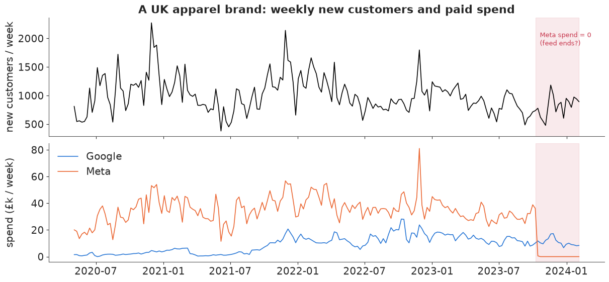
One data problem first. Meta spend drops from about £35k a week to £548 in the week ending 15 October 2023 and to exactly zero from then to the end, while new customers carry on at their usual level after the Black Friday peak. E34 and E35 found the same mid-October 2023 Meta cut-off in other brands of this dataset. A company-wide switch-off is possible, but a Meta data feed that stopped is the likelier story, and a flexible response curve would read those weeks as "zero Meta spend costs almost nothing", which would bend the curve. We stop the series at the last full week of Meta data (a "Try it yourself" item keeps the rest in).
weekly = weekly_all[weekly_all.index < feed_end].copy()
CHANNELS = ["google", "meta"]
SPEND = weekly[CHANNELS].to_numpy()
SPEND_MEAN = SPEND.mean(axis=0)
X_SPEND = SPEND / SPEND_MEAN  # 1 = the channel's average week
y_obs = weekly["FIRST_PURCHASES"].to_numpy()
T = len(weekly)
t_years = np.arange(T) / 52.18
FOURIER = np.column_stack([f(2 * np.pi * j * t_years) for j in (1, 2, 3) for f in (np.sin, np.cos)])
TREND = (t_years - t_years.mean()) / t_years.std()
idx = weekly.index
black_friday = ((idx.month == 11) & (idx.day >= 22)) | ((idx.month == 12) & (idx.day <= 3))
christmas = ((idx.month == 12) & (idx.day >= 20)) | ((idx.month == 1) & (idx.day <= 3))
HOLIDAYS = np.column_stack([black_friday, christmas]).astype(float)
print(f"{T} weeks, {idx.min().date()} -> {idx.max().date()}; average spend: "
      + ", ".join(f"{c} £{m:,.0f}" for c, m in zip(CHANNELS, SPEND_MEAN)))
print("spend range in units of an average week (min, 5%, 95%, max):")
for j, ch in enumerate(CHANNELS):
    print(f"  {ch:7s}", np.quantile(X_SPEND[:, j], [0, 0.05, 0.95, 1]).round(2))
180 weeks, 2020-05-03 -> 2023-10-08; average spend: google £9,078, meta £34,991
spend range in units of an average week (min, 5%, 95%, max):
  google  [0.   0.09 2.05 3.1 ]
  meta    [0.33 0.54 1.48 2.32]
The model
A deliberately conventional MMM, so that the only thing that changes between models is the response curve. Weekly new customers follow a negative binomial with mean
$$ \mu_t = \underbrace{\exp\big(a_0 + b_{\text{trend}}\,t + \text{Fourier}_t + \text{holidays}_t\big)}_{\text{baseline}} + \sum_{\text{channel } j} \beta_j\, f_j\big(\text{adstock}_j(x_{j})_t\big). $$
Media adds customers on top of the baseline. $\beta_j$, the customers a channel brings in an average week, gets its prior through the average cost per customer at average spend, $\text{CAC}_j = \bar{S}_j / \beta_j \sim \text{LogNormal}(\log 60, 0.8)$: £60 with a wide spread, the units a marketer would argue about. Three response curves $f$:
- Weibull: the family above, $k \sim \text{LogNormal}(0, 0.5)$, $c \sim \text{HalfNormal}(1.5)$;
- Hill: $f = \frac{x^n}{K^n + x^n} \cdot (K^n + 1)$, $K \sim \text{LogNormal}(0, 0.7)$, $n \sim \text{LogNormal}(0.3, 0.5)$ (concave or S);
- logistic saturation: normalised at $x = 1$, $\lambda \sim \text{LogNormal}(0, 1)$ (concave only).
All three normalise $f(1) = 1$, so $\beta$ means the same thing in each.
def build_mmm(y, x_spend, curve="weibull"):
    coords = {"channel": CHANNELS, "week": np.arange(len(y)), "fourier": np.arange(FOURIER.shape[1]),
              "holiday": ["black_friday", "christmas"]}
    x_jax = jnp.asarray(x_spend)
    n_ch = len(CHANNELS)
    with pm.Model(coords=coords) as model:
        theta = pm.Beta("theta", 2.0, 2.0, dims="channel")  # adstock retention per week
        cac = pm.LogNormal("cac", np.log(60.0), 0.8, dims="channel")
        beta = pm.Deterministic("beta", SPEND_MEAN / cac, dims="channel")
        theta_ = pt.specify_shape(theta, (n_ch,))
        if curve == "weibull":
            k = pm.LogNormal("k", 0.0, 0.5, dims="channel")
            c = pm.HalfNormal("c", 1.5, dims="channel")
            transform = pytensor.wrap_jax(lambda th, k_, c_: media_transform(x_jax, th, k_, c_))
            f = transform(theta_, pt.specify_shape(k, (n_ch,)), pt.specify_shape(c, (n_ch,)))
        else:
            adstock = pytensor.wrap_jax(lambda th: geometric_adstock(x_jax, th))(theta_)
            if curve == "hill":
                K = pm.LogNormal("K", 0.0, 0.7, dims="channel")
                n = pm.LogNormal("n", 0.3, 0.5, dims="channel")
                f = adstock**n / (K**n + adstock**n) * (K**n + 1)
            elif curve == "logistic":
                lam = pm.LogNormal("lam", 0.0, 1.0, dims="channel")
                sat = lambda z: (1 - pt.exp(-z)) / (1 + pt.exp(-z))  # noqa: E731
                f = sat(lam * adstock) / sat(lam)
            else:
                raise ValueError(curve)
        a0 = pm.Normal("a0", np.log(np.median(y) / 2), 0.5)
        b_trend = pm.Normal("b_trend", 0.0, 0.3)
        b_fourier = pm.Normal("b_fourier", 0.0, 0.2, dims="fourier")
        b_holiday = pm.Normal("b_holiday", 0.0, 0.5, dims="holiday")
        baseline = pm.Deterministic(
            "baseline", pt.exp(a0 + b_trend * TREND + FOURIER @ b_fourier + HOLIDAYS @ b_holiday),
            dims="week")
        mu = baseline + f @ beta
        alpha = pm.Gamma("alpha", 2.0, 0.05)
        pm.NegativeBinomial("y", mu=mu, alpha=alpha, observed=y, dims="week")
    return model


model_weibull = build_mmm(y_obs, X_SPEND, "weibull")
print(model_weibull.point_logps())
{'theta': np.float64(-1.96), 'cac': np.float64(-1.55), 'k': np.float64(-0.51), 'c': np.float64(-1.45), 'a0': np.float64(-0.23), 'b_trend': np.float64(0.29), 'b_fourier': np.float64(4.14), 'b_holiday': np.float64(-0.45), 'alpha': np.float64(-0.61), 'y': np.float64(-1335.94)}Before sampling, check the wrapped Op's gradient the PyTensor way: verify_grad compares
the symbolic (here: JAX) gradient with finite differences along random directions.
transform_only = pytensor.wrap_jax(lambda th, k_, c_: media_transform(jnp.asarray(X_SPEND), th, k_, c_))
pytensor.gradient.verify_grad(
    lambda th, k_, c_: transform_only(th, k_, c_).sum(),
    [np.array([0.4, 0.2]), np.array([1.7, 0.8]), np.array([0.3, 1e-5])],
    rng=np.random.default_rng(RANDOM_SEED), eps=1e-7)
print("verify_grad passed (one input sits in the series branch, c = 1e-5)")
verify_grad passed (one input sits in the series branch, c = 1e-5)
Prior predictive: a prior on shapes
With a flexible family, the prior on $(k, c)$ is a prior on shapes, so it is worth looking at in those terms: how often each shape class appears on the data range, and what the curves look like in customers per week.
with model_weibull:
    prior = pm.sample_prior_predictive(1000, random_seed=RANDOM_SEED)
pk = prior.prior["k"].values.reshape(-1, 2)
pc = prior.prior["c"].values.reshape(-1, 2)
pb = prior.prior["beta"].values.reshape(-1, 2)
prior_classes = shape_class(pk[:, 0], pc[:, 0])
print("prior shape classes on 0 <= x <= 2.5:",
      {n: round(float(np.mean(prior_classes == i)), 2) for i, n in enumerate(SHAPE_NAMES)})
fig, axes = plt.subplots(1, 2, figsize=(12, 4))
xg = np.linspace(0, X_RANGE, 200)
for i in range(80):
    axes[0].plot(xg, pb[i, 1] * weibull_np(xg, pk[i, 1], pc[i, 1]), color=BLUE, lw=0.6, alpha=0.4)
axes[0].set(xlabel="Meta spend (1 = average week)", ylabel="customers / week from Meta",
            title="Prior response curves (80 draws)", ylim=(0, 3000))
y_prior = prior.prior_predictive["y"].values.reshape(-1, T)
for q_lo, q_hi, a in [(0.05, 0.95, 0.25), (0.25, 0.75, 0.4)]:
    axes[1].fill_between(idx, *np.quantile(y_prior, [q_lo, q_hi], axis=0), color=GREY, alpha=a, lw=0)
axes[1].plot(idx, y_obs, color="k", lw=1)
axes[1].set(ylabel="new customers / week", title="Prior predictive (50% and 90%) vs data", ylim=(0, 6000))
axes[1].xaxis.set_major_locator(plt.matplotlib.dates.YearLocator())
axes[1].xaxis.set_major_formatter(plt.matplotlib.dates.DateFormatter("%Y"))
prior shape classes on 0 <= x <= 2.5: {'concave': 0.52, '≈ linear': 0.0, 'convex': 0.02, 'S-shaped': 0.46}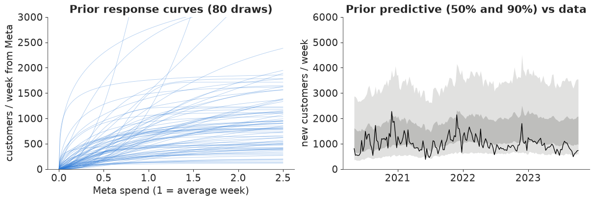
The prior is split roughly evenly between concave and S-shaped curves on the data range; convex and near-linear curves are rare, because they need $c$ close to zero, where HalfNormal(1.5) puts little mass. That is a choice worth stating: this prior leans towards saturation. Response curves range from a few dozen to a few thousand customers a week, and the prior predictive covers the data without being absurd.
7 · Fake data: when the family is too narrow
Before the real data, a check with a known answer. Keep the brand's real spend (so the design is realistic), and simulate new customers with Google S-shaped (a Hill curve, $K = 1.2$, $n = 3$, 350 customers in an average week) and Meta as a pure power curve $300\,x^{0.6}$ (concave, never saturating), adstock retention 0.5 and 0.3, and negative binomial noise close to what the real data turn out to have. Then fit all three models. The Hill curve is not in the Weibull family (only approximated, section 4); the power curve is, at $c = 0$, a corner the prior makes unlikely; and the logistic model cannot make an S at all.
THETA_TRUE = np.array([0.5, 0.3])
ad_true = np.asarray(geometric_adstock(jnp.asarray(X_SPEND), jnp.asarray(THETA_TRUE)))
truth_curves = {"google": lambda x: 350 * hill_np(x, 1.2, 3.0) / hill_np(1.0, 1.2, 3.0),
                "meta": lambda x: 300 * x**0.6}
baseline_true = np.exp(np.log(500) + 0.15 * TREND + FOURIER @ np.array([0.1, -0.05, 0.05, 0, 0, 0.03])
                       + HOLIDAYS @ np.array([0.5, 0.2]))
mu_true = baseline_true + truth_curves["google"](ad_true[:, 0]) + truth_curves["meta"](ad_true[:, 1])
ALPHA_TRUE = 35.0
y_fake = rng.negative_binomial(ALPHA_TRUE, ALPHA_TRUE / (ALPHA_TRUE + mu_true))
print(f"simulated weekly customers: mean {y_fake.mean():.0f}, media share "
      f"{(mu_true - baseline_true).sum() / mu_true.sum():.0%}")


def fit(model, **kw):
    t0 = time.perf_counter()
    idata = pm.sample(model=model, random_seed=RANDOM_SEED, progressbar=False,
                      var_names=[v.name for v in model.free_RVs] + ["beta"], **kw)
    idata.attrs["seconds"] = time.perf_counter() - t0
    n_div = int(idata.sample_stats["diverging"].sum())
    rhat = float(az.summary(idata, var_names=[v.name for v in model.free_RVs])["r_hat"].max())
    print(f"  {idata.attrs['seconds']:.0f} s, {n_div} divergences, max r_hat {rhat:.3f}")
    return idata


fake_fits = {}
for curve in ("weibull", "hill", "logistic"):
    print(curve)
    fake_fits[curve] = fit(build_mmm(y_fake, X_SPEND, curve))
simulated weekly customers: mean 1193, media share 56%
weibull
  12 s, 0 divergences, max r_hat 1.016
hill
  9 s, 0 divergences, max r_hat 1.005
logistic
7 s, 0 divergences, max r_hat 1.009
To compare the three models' curves we need each posterior's response curve and its slope.
The Weibull ones come straight from the JAX function: jax.vmap over posterior draws for the
curve and jax.vmap(jax.grad(...)) for the slope, with no hand-derived derivative.
def curve_draws(idata, curve, j, x, n=1000):
    """Posterior response curves (draw, x) in customers/week for channel j, and slope at x = 1."""
    post = az.extract(idata, num_samples=n, random_seed=RANDOM_SEED)
    beta = post["beta"].values[j]
    if curve == "weibull":
        k, c = post["k"].values[j], post["c"].values[j]
        f = jax.vmap(weibull, in_axes=(None, 0, 0))(jnp.asarray(x), k, c)
        slope = jax.vmap(jax.grad(weibull), in_axes=(None, 0, 0))(1.0, k, c)
    elif curve == "hill":
        K, n_ = post["K"].values[j][:, None], post["n"].values[j][:, None]
        hill = lambda z: z**n_ / (K**n_ + z**n_) * (K**n_ + 1)  # noqa: E731
        f, slope = hill(x[None]), ((hill(1.0 + 1e-5) - hill(1.0 - 1e-5)) / 2e-5)[:, 0]
    else:
        lam = post["lam"].values[j][:, None]
        sat = lambda z: (1 - np.exp(-lam * z)) / (1 + np.exp(-lam * z)) / logistic_np(1.0, lam)  # noqa: E731
        f, slope = sat(x[None]), ((sat(1.0 + 1e-5) - sat(1.0 - 1e-5)) / 2e-5)[:, 0]
    return beta[:, None] * np.asarray(f), beta * np.asarray(slope)


CURVE_COLORS = {"weibull": BLUE, "hill": AQUA, "logistic": ORANGE}
xg = np.linspace(0, 3, 200)
fig, axes = plt.subplots(1, 2, figsize=(13, 4.5))
rows = []
for j, (ax, ch) in enumerate(zip(axes, CHANNELS)):
    for curve, idata in fake_fits.items():
        f, slope = curve_draws(idata, curve, j, xg)
        lo, md, hi = np.quantile(f, [0.05, 0.5, 0.95], axis=0)
        ax.fill_between(xg, lo, hi, color=CURVE_COLORS[curve], alpha=0.15, lw=0)
        ax.plot(xg, md, color=CURVE_COLORS[curve], lw=2, label=curve)
        rows.append({"channel": ch, "model": curve, "customers at x=1": np.median(f[:, np.searchsorted(xg, 1.0)]),
                     "marginal at x=1 (median)": np.median(slope),
                     "marginal 90% interval": f"{np.quantile(slope, 0.05):.0f} - {np.quantile(slope, 0.95):.0f}"})
    true_f = truth_curves[ch](xg)
    ax.plot(xg, true_f, "k--", lw=1.5, label="truth")
    rows.append({"channel": ch, "model": "TRUTH", "customers at x=1": truth_curves[ch](1.0),
                 "marginal at x=1 (median)": (truth_curves[ch](1.001) - truth_curves[ch](0.999)) / 0.002,
                 "marginal 90% interval": ""})
    ax2 = ax.twinx()
    ax2.hist(ad_true[:, j], bins=30, range=(0, 3), color=GREY, alpha=0.25)
    ax2.set_yticks([])
    ax.set(xlabel="adstocked spend (1 = average week); grey: weeks observed", ylabel="customers / week",
           title=f"{ch.title()}: truth is {'S-shaped (Hill)' if ch == 'google' else 'a power curve'}")
    ax.set_zorder(ax2.get_zorder() + 1)
    ax.patch.set_visible(False)
axes[0].legend(fontsize=8, loc="upper left")
display(pd.DataFrame(rows).set_index(["channel", "model"]).round(0));
| customers at x=1 | marginal at x=1 (median) | marginal 90% interval | ||
|---|---|---|---|---|
| channel | model | |||
| weibull | 369.0 | 514.0 | 401 - 672 | |
| hill | 360.0 | 537.0 | 416 - 672 | |
| logistic | 449.0 | 430.0 | 352 - 498 | |
| TRUTH | 350.0 | 665.0 | ||
| meta | weibull | 489.0 | 214.0 | 106 - 350 |
| hill | 488.0 | 213.0 | 110 - 333 | |
| logistic | 386.0 | 203.0 | 70 - 340 | |
| TRUTH | 300.0 | 180.0 |
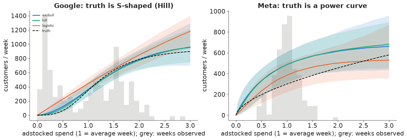
Reading the fake-data check. (The marginal effect is in customers per week per extra "average week" of spend; divide the average spend by it to get the marginal cost per customer.)
- Google, S-shaped truth. The Weibull and Hill models both bend the right way, flat at low spend and steep through the middle, and follow the truth closely wherever there are weeks of data. The logistic model cannot start flat, so it draws a nearly straight line through the same weeks. The table shows the consequence: it overstates the customers Google brings in an average week (about 450 against a true 350) and understates the marginal return, with a 90% interval that excludes the truth. A family that is too narrow gives a confident wrong answer, not an uncertain one. The flexible models also understate the steepest slope of the S a little (the truth sits at the top of their intervals): a sharp S gets smoothed out by noise and a prior that prefers gentler curves.
- Meta, power truth. All three recover the slope where the data are (marginal about 200 against a true 180), and all three overstate the level, by 30-60%. This is not about curve families. Meta is always on, between 0.4 and 1.6 of an average week, so no week shows what zero Meta spend would look like, and the level of the curve trades off against the baseline. For an always-on channel, the marginal return is measured; the average return (and so the "average CAC" or ROI) is an extrapolation to zero spend. Above the data, the Weibull fit bends towards saturation because its prior on $c$ expects some, and with no data there, the prior wins: section 4's lesson again, inside a posterior.
real_fits = {}
for curve in ("weibull", "hill", "logistic"):
    print(curve)
    real_models = build_mmm(y_obs, X_SPEND, curve)
    real_fits[curve] = fit(real_models)
    pm.compute_log_likelihood(real_fits[curve], model=real_models, progressbar=False)
display(az.summary(real_fits["weibull"], var_names=["theta", "cac", "beta", "k", "c", "alpha"]))
weibull
9 s, 0 divergences, max r_hat 1.010
hill
9 s, 3 divergences, max r_hat 1.011
logistic
6 s, 0 divergences, max r_hat 1.002
| mean | sd | eti89_lb | eti89_ub | ess_bulk | ess_tail | r_hat | mcse_mean | mcse_sd | |
|---|---|---|---|---|---|---|---|---|---|
| theta[google] | 0.194 | 0.128 | 0.04 | 0.43 | 5842 | 2672 | 1.00 | 0.0017 | 0.0028 |
| theta[meta] | 0.0443 | 0.029 | 0.0088 | 0.097 | 4434 | 2193 | 1.00 | 0.00039 | 0.00055 |
| cac[google] | 80 | 27 | 49 | 130 | 956 | 1391 | 1.00 | 0.9 | 1.1 |
| cac[meta] | 56.2 | 5.3 | 49 | 66 | 808 | 1171 | 1.01 | 0.19 | 0.16 |
| beta[google] | 124 | 36 | 71 | 180 | 956 | 1391 | 1.00 | 1.2 | 0.68 |
| beta[meta] | 628 | 57 | 530 | 720 | 808 | 1171 | 1.01 | 2 | 1.3 |
| k[google] | 2.37 | 0.91 | 1.1 | 3.9 | 1462 | 1341 | 1.00 | 0.023 | 0.016 |
| k[meta] | 1.54 | 0.26 | 1.2 | 2 | 1160 | 1747 | 1.00 | 0.0075 | 0.0051 |
| c[google] | 0.63 | 0.27 | 0.27 | 1.1 | 1482 | 1164 | 1.00 | 0.0064 | 0.007 |
| c[meta] | 0.42 | 0.232 | 0.067 | 0.81 | 1518 | 1228 | 1.00 | 0.0056 | 0.0033 |
| alpha | 42.4 | 5.2 | 35 | 51 | 4330 | 2890 | 1.00 | 0.079 | 0.089 |
with warnings.catch_warnings():
    warnings.filterwarnings("ignore", message="Estimated shape parameter of Pareto")
    cmp = az.compare(real_fits, round_to=1)
    for curve, idata in real_fits.items():
        k_hat = np.asarray(az.loo(idata, pointwise=True).pareto_k)
        worst_week = idx[int(np.argmax(k_hat))].date()
        print(f"{curve:8s}: {int((k_hat > 0.7).sum())} weeks with Pareto k > 0.7 "
              f"(worst {k_hat.max():.2f}, week ending {worst_week})")
display(cmp[["elpd", "p", "elpd_diff", "dse", "weight"]])
for idata in real_fits.values():
    del idata["log_likelihood"]  # LOO is done; the pointwise matrix is not needed any more
weibull : 0 weeks with Pareto k > 0.7 (worst 0.68, week ending 2020-11-22)
hill    : 0 weeks with Pareto k > 0.7 (worst 0.63, week ending 2020-11-29)
logistic: 0 weeks with Pareto k > 0.7 (worst 0.52, week ending 2020-11-22)
| elpd | p | elpd_diff | dse | weight | |
|---|---|---|---|---|---|
| weibull | -1168.8 | 14.9 | 0.0 | 0.0 | 1.0 |
| hill | -1169.4 | 14.5 | -0.5 | 0.5 | 0.0 |
| logistic | -1173.6 | 13.0 | -4.7 | 2.3 | 0.0 |
The sampler has no trouble with the Weibull model (no divergences, r_hat at most 1.01; the Hill model has a few divergences). LOO puts the Weibull and Hill models level and the logistic model behind by about 5 points of elpd, two standard errors of the difference. That is moderate, not overwhelming, evidence against the concave-only family, and no week has a Pareto $\hat{k}$ above 0.7, so the estimates are reliable. Where do the models differ?
fig, axes = plt.subplots(1, 2, figsize=(13, 4.5))
real_rows = []
post_w = az.extract(real_fits["weibull"], num_samples=1000, random_seed=RANDOM_SEED)
theta_med = np.median(post_w["theta"].values, axis=1)
ad_med = np.asarray(geometric_adstock(jnp.asarray(X_SPEND), jnp.asarray(theta_med)))
for j, (ax, ch) in enumerate(zip(axes, CHANNELS)):
    for curve, idata in real_fits.items():
        f, slope = curve_draws(idata, curve, j, xg)
        lo, md, hi = np.quantile(f, [0.05, 0.5, 0.95], axis=0)
        ax.fill_between(xg, lo, hi, color=CURVE_COLORS[curve], alpha=0.15, lw=0)
        ax.plot(xg, md, color=CURVE_COLORS[curve], lw=2, label=curve)
        beta = az.extract(idata, var_names="beta", num_samples=1000, random_seed=RANDOM_SEED).values[j]
        real_rows.append({"channel": ch, "model": curve,
                          "average CAC £ (median)": np.median(SPEND_MEAN[j] / beta),
                          "marginal CAC £ (median)": np.median(SPEND_MEAN[j] / slope),
                          "marginal CAC 90% interval": "£{:.0f} - £{:.0f}".format(
                              *np.quantile(SPEND_MEAN[j] / slope, [0.05, 0.95]))})
    lo_obs, hi_obs = np.quantile(ad_med[:, j], [0.0, 1.0])
    for edge in (lo_obs, hi_obs):
        ax.axvline(edge, color=GREY, ls=":", lw=1)
    ax.axvspan(0, lo_obs, color=GREY, alpha=0.08)
    ax.axvspan(hi_obs, 3, color=GREY, alpha=0.08)
    ax.set(xlabel="adstocked spend (1 = average week); shaded: never observed",
           ylabel="customers / week", title=f"{ch.title()}: posterior response curves (90% bands)")
axes[0].legend(fontsize=8, loc="upper left")
display(pd.DataFrame(real_rows).set_index(["channel", "model"]).round(0));
| average CAC £ (median) | marginal CAC £ (median) | marginal CAC 90% interval | ||
|---|---|---|---|---|
| channel | model | |||
| weibull | 75.0 | 48.0 | £30 - £91 | |
| hill | 74.0 | 52.0 | £32 - £96 | |
| logistic | 81.0 | 91.0 | £62 - £167 | |
| meta | weibull | 56.0 | 46.0 | £40 - £53 |
| hill | 56.0 | 46.0 | £40 - £54 | |
| logistic | 51.0 | 53.0 | £47 - £60 |
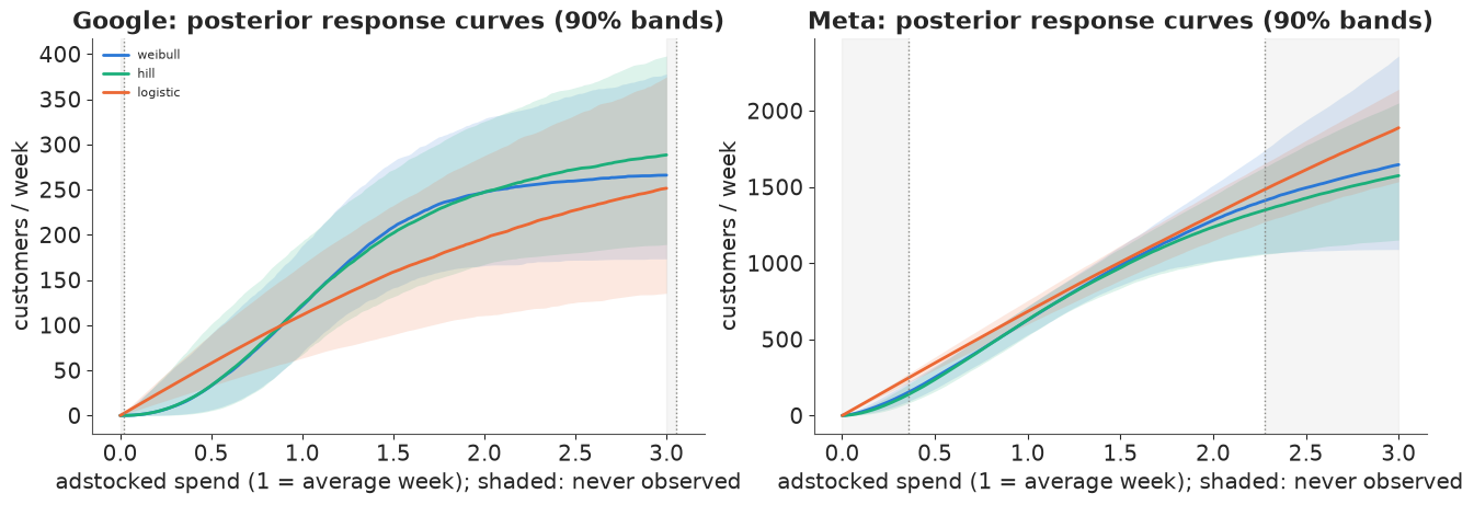
The two flexible models agree with each other almost exactly, and they differ from the logistic model where it matters for a decision.
- Google is S-shaped in the flexible models: little response below about half an average week, then a steep rise, then flattening above twice the average. The logistic model draws a concave curve through the same weeks. At current spend the flexible models put Google's marginal cost per customer at about £50, the logistic model at about £90, with 90% intervals that overlap only between about £60 and £90. The two families would give opposite advice on moving budget into Google.
- Meta's curves are nearly identical in all three models over the observed range (0.36 to 2.3 of an average week) and nearly straight; the flexible models' marginal CAC (£46) is a little below their average CAC (£56).
One more sensitivity worth knowing about: the week ending 15 October 2023, with £549 of Meta spend, is not in the data. With it included (an earlier draft of this notebook did that), a single week at 2% of normal Meta spend moved Meta's average CAC from £56 to about £85 and the shape parameters with it. Curves are learned from the extremes of spend, so the extremes deserve the most scrutiny.
Where do the posteriors sit on the shape map, and which shape class do they give each channel?
fig, axes = plt.subplots(1, 2, figsize=(12, 4.6))
shape_rows = {}
for j, (ax, ch) in enumerate(zip(axes, CHANNELS)):
    draw_shape_map(ax, labels=(j == 0))
    k_d, c_d = post_w["k"].values[j], post_w["c"].values[j]
    ax.scatter(pk[:400, j], pc[:400, j], s=3, color=GREY, alpha=0.4, label="prior")
    ax.scatter(k_d, c_d, s=4, color=BLUE if j == 0 else ORANGE, alpha=0.5, label="posterior")
    ax.set(xlim=(kg[0], kg[-1]), ylim=(cg[0], cg[-1]), title=f"{ch.title()}: posterior on the shape map")
    ax.legend(fontsize=8, loc="lower left")
    x_obs_max = ad_med[:, j].max()
    x_star = inflection(k_d, c_d)
    shape_rows[ch] = {**{n: float(np.mean(shape_class(k_d, c_d) == i)) for i, n in enumerate(SHAPE_NAMES)},
                      "inflection inside observed range": float(np.mean(
                          (x_star > ad_med[:, j].min()) & (x_star < x_obs_max))),
                      "median inflection x*": float(np.median(x_star[np.isfinite(x_star)])),
                      "observed range": f"{ad_med[:, j].min():.2f} - {x_obs_max:.2f}"}
display(pd.DataFrame(shape_rows).T.round(2));
| concave | ≈ linear | convex | S-shaped | inflection inside observed range | median inflection x* | observed range | |
|---|---|---|---|---|---|---|---|
| 0.036 | 0.003 | 0.003 | 0.958 | 0.96 | 0.935824 | 0.02 - 3.06 | |
| meta | 0.004 | 0.036 | 0.057 | 0.903 | 0.924 | 0.887844 | 0.36 - 2.27 |
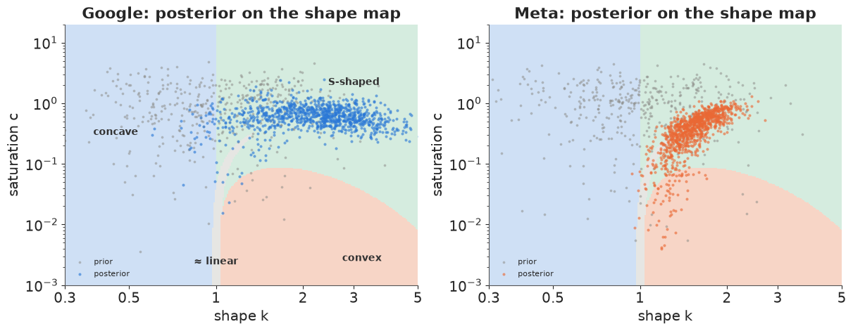
- Both channels move to the S-shaped region, from a prior that gave S-curves about 46%: the posterior probability of an S with its inflection inside the observed range is above 0.9 for both, with the inflection near an average week.
- Meta's cloud is tight and runs down into the convex region: with its lowest weeks at 0.36 of average spend, the data cannot distinguish "an S whose lower bend is below 0.36" from "convex"; the posterior hedges between them.
- Google's shape is less certain ($k$ between about 1 and 4), but it is S-shaped in almost every draw.
Should we believe S-shaped curves?
An S-curve says there is a threshold: spend below it is mostly wasted. Before a CFO hears that, two alternative explanations should be ruled out:
- Time, not spend. Google spend was tiny in 2020-21 and grew over the following years (see the data plot). The flat start of its S is learned from those early weeks, when many other things were different. A linear trend and a yearly season in the baseline cannot absorb all of that, and the S may partly be a story about 2020.
- Spend chases demand. When a budget algorithm or a planner raises spend in weeks that were going to sell well anyway, high-spend weeks have high sales for other reasons, and the curve steepens at the top. That is the endogeneity E32 built a likelihood for. A concave family hides such a distortion (it cannot bend upwards, so the distortion leaks into other parameters); a flexible family exposes it. Flexibility does not fix confounding, it makes it visible.
The flexible model is the right tool for asking the question, not the last word on the answer. A holdout or geo experiment (E34) is what settles it.
A posterior predictive check to finish: do the fitted models reproduce the weekly series?
fig, axes = plt.subplots(2, 1, figsize=(12, 6), sharex=True)
for ax, curve in zip(axes, ("weibull", "logistic")):
    model = build_mmm(y_obs, X_SPEND, curve)
    with model:
        ppc = pm.sample_posterior_predictive(real_fits[curve], random_seed=RANDOM_SEED, progressbar=False)
    y_rep = ppc.posterior_predictive["y"].values.reshape(-1, T)
    lo, hi = np.quantile(y_rep, [0.05, 0.95], axis=0)
    ax.fill_between(idx, lo, hi, color=CURVE_COLORS[curve], alpha=0.25, lw=0, label="90% predictive")
    ax.plot(idx, y_obs, color="k", lw=1, label="observed")
    coverage = np.mean((y_obs >= lo) & (y_obs <= hi))
    ax.set(ylabel="new customers / week", title=f"{curve}: 90% interval covers {coverage:.0%} of weeks")
    ax.legend(fontsize=8, loc="upper left")
    del ppc, y_rep
alpha_med = float(real_fits["weibull"].posterior["alpha"].median())
print(f"NB alpha = {alpha_med:.0f}: at 1,000 customers/week the sd is "
      f"{np.sqrt(1000 + 1000**2 / alpha_med):.0f} ({np.sqrt(1000 + 1000**2 / alpha_med) / 10:.0f}%)")
NB alpha = 42: at 1,000 customers/week the sd is 157 (16%)
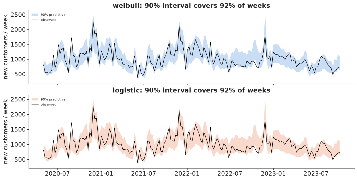
Both models track the series, with 90% intervals covering 93% of weeks, so a time-series PPC cannot tell them apart. The difference LOO found is spread thinly over many weeks: it concerns the shape of the curves, which barely moves the total. That is typical. In MMMs, the part of the model a decision depends on is often the part a fit plot says least about.
9 · Performance: a JAX node inside a Numba graph, or all JAX?
By default nutpie compiles the model with Numba and calls the wrapped JAX function as a single
node, in Numba's "object mode" (a Python call, hence the warning we silenced at the top), with a
separate call for its gradient. The whole model can also be compiled to JAX, in which case
wrap_jax's node is inlined into one XLA program (E09 explains why this works for wrap_jax and
not for a hand-written Op). Time one log-density + gradient evaluation each way, then sample
with the JAX backend.
def time_logp_grad(model, mode, reps=300):
    logp = model.logp()
    fn = pytensor.function(model.value_vars, [logp, *pt.grad(logp, model.value_vars)], mode=mode)
    point = model.initial_point()
    args = [point[v.name] for v in model.value_vars]
    fn(*args)  # compile / warm up
    t0 = time.perf_counter()
    for _ in range(reps):
        fn(*args)
    return 1e6 * (time.perf_counter() - t0) / reps


timings = {"Numba graph + JAX node": time_logp_grad(model_weibull, "NUMBA"),
           "whole model in JAX": time_logp_grad(model_weibull, "JAX")}
for name, us in timings.items():
    print(f"{name:24s} {us:7.0f} µs per logp + gradient")
print("sampling, Numba backend (section 8):", f"{real_fits['weibull'].attrs['seconds']:.0f} s")
idata_jax = fit(model_weibull, backend="jax", compile_kwargs={"gradient_backend": "jax"})
jax_vs_numba = float(np.abs(idata_jax.posterior["k"].median(["chain", "draw"])
                            - real_fits["weibull"].posterior["k"].median(["chain", "draw"])).max())
print(f"largest difference in posterior median k between backends: {jax_vs_numba:.2f}")
del idata_jax
jax.clear_caches()
Numba graph + JAX node       115 µs per logp + gradient
whole model in JAX            35 µs per logp + gradient
sampling, Numba backend (section 8): 9 s
  5 s, 0 divergences, max r_hat 1.003
largest difference in posterior median k between backends: 0.02
Compiling the whole model to JAX makes one log-density + gradient about three times faster (the object-mode call into JAX costs more than the arithmetic), and sampling takes about half the time; the two backends give the same posterior. With 180 weeks and two channels both are fast. The whole-model JAX route pays off more with larger models (many geos, E33) or on a GPU, where float32 is the norm, which is one more reason section 3 made the function float32-safe.
Summary
- The response family is a prior, and a strong one: it decides which shapes have any probability at all. Hill, logistic and power curves agree at the reference spend and disagree by a factor of four on the marginal return (section 1).
- One family, three behaviours. $f(x) = (1 - e^{-cx^k})/(1 - e^{-c})$ contains power curves ($c = 0$), concave saturation ($k \le 1$) and S-curves ($k > 1$, inflection at $((k-1)/(ck))^{1/k}$), and moves between them smoothly, which NUTS needs (section 2).
- A custom JAX function needs the same care as any numerical code:
expm1plus a series switch for $c \to 0$, the double-wheretrick for zero spend, float32 in mind, and unit tests for limits, gradients and curvature (section 3). - It imitates the standard curves to about 1% over the data range, far below weekly noise.
Batched fits with
vmapcheck that in a few seconds and translate a Hill prior into $(k, c)$. Outside the data, families diverge, and so do their decisions (sections 4-5). - In a Bayesian MMM the flexible family recovers an S-shaped truth where a concave-only model gives a confident wrong marginal return. For an always-on channel only the marginal return is measured; the level is an extrapolation (section 7).
- On a real brand, the flexible models find S-curves for both channels and roughly halve Google's marginal cost per customer relative to the logistic model, which LOO ranks lower. Whether the S is real or reflects time trends and demand-chasing spend is a question for an experiment (section 8).
Try it yourself
- Keep the "feed ends" weeks. Refit on
weekly_all(Meta spend near zero or zero for the last 17 weeks). How do Meta's average and marginal CAC and its position on the shape map change? Is the result a better or a worse description of the brand if the zeros are a lost feed? - Use the translated Hill prior. Replace the independent priors on $k$ and $c$ by the
bivariate normal on $(\log k, \log c)$ from section 5 (
pm.MvNormalon a length-2 vector per channel, exponentiated). Which conclusions in section 8 depend on the shape prior? - Weibull adstock. Robyn's other use of the Weibull family is for the adstock: lag
weights $w_\ell \propto$ Weibull PDF or survival function at lag $\ell$, so the peak effect
can come weeks after the spend. Write it as a JAX convolution (
jnp.convolveor alax.scanover a lag window), put it inmedia_transform, and compare with geometric adstock by LOO.