Every GPU number here is a stored table, measured once on an RTX 3090 Ti and loaded from
results/E87/. A normal run uses the CPU only and never starts a GPU.
The question
US rules single out flights that are late again and again. Under 14 CFR 399.81(c), a chronically delayed flight is a domestic flight operated at least 10 times in a month that arrives more than 30 minutes late, or is cancelled, more than half the time in that month. A carrier's departures in one city-pair market within 30 minutes of the most frequent scheduled time count as one flight, and holding such a flight out for more than four consecutive months is a violation.
Suppose the research lead of a passenger-rights charity wants a monthly watch list: the 50 flights most likely to be flagged next month. A contractor quotes a flight-level model fitted to two years of every US flight, "two hours on one GPU, from a published rate". The charity's own analyst says a table of counts will do. The lead has one workstation for one night a month, about 8 hours. Should the charity approve the quote, buy something smaller, or refuse? And would the bigger model change the list?
The first half of the question is about pricing a model. A gradient-based sampler such as NUTS (Hoffman & Gelman 2014) or ChEES (Hoffman, Radul & Sountsov 2021) spends nearly all its time evaluating the gradient of the log density, so the running time of a fit is
$$\text{time} = (\text{time per gradient}) \times (\text{gradients per fit}) \times (\text{fits}),$$
and the model must also fit in memory and keep enough digits in its arithmetic. The contractor took the rate of E86's forest model and multiplied it by the size of this data. We check whether that rate transfers, what gradient count the quote assumes, how many fits a test needs, and which walls a rate cannot see.
The second half is about value. We build a ladder of forecasts of rising cost:
- R0, persistence: a flight flagged last month will be flagged again;
- R1, a beta-binomial count of each flight's late operations, shrunk towards its carrier;
- R2, a hierarchical beta-binomial on flight x month cells, with effects for origin, destination, flight and month;
- R3, the contractor's model: a Bernoulli logit on every one of the 14 million rows, with five lookups per row.
A dearer model is worth buying only if it scores better than the cheaper one or changes the list. R0 and R1 run on all carriers in under a second. R2 is fitted on one carrier, because a national fit does not fit in a reader's run. R3 is priced and never fitted.
What counts as a flag
Flagged below means a flight that met this test in a month as we code it: directions kept apart, diversions not counted as late, and flights linked across months by our own rule. It is our estimate, not DOT's, so the list says "likely to be flagged"; carriers, airports and flights carry integer codes, and the carrier of part 6 is called the mid-size carrier.
The plan
| part | question | tool |
|---|---|---|
| 1 | What does the quote assume, and what would R3 cost? | measured gradients, an iso-cost map |
| 2 | What do the flights look like? | flight x month cells, flags per month |
| 3 | Does a rate carry over from one model to another? | time_gradient on five cost shapes, CPU and GPU |
| 4 | Which walls does a rate not show? | a VRAM grid, the sampler's own memory, float32 spacing |
| 5 | How good are the counting rules? | persistence and a beta-binomial, all carriers |
| 6 | What does a hierarchical model add on one carrier? | R2 in PyMC with nutpie, with the month redrawn |
| 7 | Does the bigger model change the list? | a decision rule fixed before scoring |
| 8 | What should the charity be told? | a price table, and a quote that can be checked |
import os

for name in ("OPENBLAS_NUM_THREADS", "OMP_NUM_THREADS", "MKL_NUM_THREADS"):
    os.environ.setdefault(name, "1")  # before NumPy: one BLAS thread per chain
os.environ["JAX_PLATFORMS"] = "cpu"  # the GPU numbers here are stored: a reader's run never starts one

import contextlib
import gc
import logging
import time
import warnings

import arviz as az
import jax
import jax.numpy as jnp
import matplotlib.pyplot as plt
import numpy as np
import nutpie
import pandas as pd
import pymc as pm
import pytensor
import pytensor.tensor as pt
import xarray as xr
from jax.flatten_util import ravel_pytree
from jax.scipy.special import gammaln as jax_gammaln
from matplotlib.colors import LogNorm
from matplotlib.lines import Line2D
from matplotlib.patches import Patch, Rectangle
from matplotlib.ticker import FuncFormatter, NullFormatter
from pymc.sampling.jax import get_jaxified_logp
from scipy import stats
from scipy.special import betaln, expit, gammaln

from pymc_challenges import data
from pymc_challenges.bigrun import PreflightError, Store, banner, estimated, extrapolated, git_hash, measured, time_gradient

RANDOM_SEED = 87
rng = np.random.default_rng(RANDOM_SEED)
az.style.use("arviz-variat")
logging.getLogger("pymc").setLevel(logging.WARNING)
warnings.filterwarnings("ignore", message=".*Explicitly requested dtype.*")
jax.config.update("jax_enable_x64", False)  # importing PyMC switches x64 on

LEVEL = os.environ.get("PYMC_CHALLENGES_RUN", "").strip().lower() or "small"
if LEVEL != "small":
    raise PreflightError(f"PYMC_CHALLENGES_RUN={LEVEL!r}: E87 has one level, small. The row-level run was "
                         "priced and never made, so there is nothing to replay or scale up.")
assert jax.default_backend() == "cpu", "this notebook never starts a GPU"

CORES = len(os.sched_getaffinity(0)) if hasattr(os, "sched_getaffinity") else os.cpu_count()
CHAINS_AT_ONCE = min(4, CORES)
TUNE, DRAWS = 1000, 1000  # nutpie's default 400 tuning steps is not assumed: see section 6
TARGETS = (15, 18, 21)  # 2025-04, 2025-07, 2025-10 as month numbers, with 2024-01 as 0
TARGET_NAMES = {15: "2025-04", 18: "2025-07", 21: "2025-10"}
WINDOW = 12  # months of history behind each list
LIST_SIZE, NEEDED = 10, 8  # one carrier's list, and the overlap the rung rule asks for
MEASURED, EXTRA, ALARM, CALM, MUTED = "#0b6e8a", "#a85a00", "#b2182b", "#2a7f62", "#8a8a8a"
RUNG_COLOUR = {"R0": "#8a8a8a", "R1": "#0b6e8a", "R2": "#b2182b"}
PRICE = {}


@contextlib.contextmanager
def stage(name):
    """Add the time spent in this block to the price table printed at the end."""
    start = time.perf_counter()
    yield
    PRICE[name] = PRICE.get(name, 0.0) + time.perf_counter() - start


store = Store("E87")
pilot = store.load_json("pilot_2026-11-02")  # the GPU pilot: see plans/large/E87.md section 13
extra_gpu = store.load_json("gpu_rows_2026-11-02")  # rows 2, 3 and a month of rows on the GPU
summary = store.load_json("data_summary")  # counts over all 24 files; names no carrier, airport or tail
jobs = pilot["jobs"]
print(f"{CORES} cores here: {CHAINS_AT_ONCE} chains at once. JAX backend: {jax.default_backend()}.")
2 cores here: 2 chains at once. JAX backend: cpu.
banner(wall_time=measured("12-13", "min on 2 cores, builds of 2026-11-02"),
       peak_ram=measured("2.3-2.5", "GB, whole process tree, across builds"),
       peak_vram=measured(0, "GB in this run: every GPU number is a stored table"),
       disk=measured(2.8, "MB in data/, and under 0.2 MB of JSON in results/E87/"),
       download=measured(0, "MB: the tables are built by tools/build_e87_data.py from 710 MB of BTS zips"),
       precision=measured("float32 for gradient timing, float64 for the fits", ""),
       chains=measured(4, "chains, 1,000 draws, 3 fits of R2"),
       hardware=measured("Ryzen 5950X on 2 cores; stored GPU tables from an RTX 3090 Ti", ""),
       build_date=measured("2026-11-02", ""),
       git_hash=measured(git_hash() or "unknown", ""),
       smaller_machine=estimated("this is the small problem: no larger level exists", ""))
| Value | Status | |
|---|---|---|
| Wall time | 12-13 min on 2 cores, builds of 2026-11-02 | measured |
| Peak RAM | 2.3-2.5 GB, whole process tree, across builds | measured |
| Peak VRAM | 0 GB in this run: every GPU number is a stored table | measured |
| Disk | 2.8 MB in data/, and under 0.2 MB of JSON in results/E87/ | measured |
| Download size | 0 MB: the tables are built by tools/build_e87_data.py from 710 MB of BTS zips | measured |
| Precision | float32 for gradient timing, float64 for the fits | measured |
| Chains | 4 chains, 1,000 draws, 3 fits of R2 | measured |
| Hardware | Ryzen 5950X on 2 cores; stored GPU tables from an RTX 3090 Ti | measured |
| Build date | 2026-11-02 | measured |
| Git hash | ba47bc242e56-dirty | measured |
| On a smaller machine | this is the small problem: no larger level exists | estimated |
1 · The price, before anything else
The contractor's sum is one line: E86's rate of 0.336 ns per chain and data cell, times 14 million rows, times 32 chains, gives about 0.15 s a gradient, and two hours of that is the quote. We measured the row-level model R3 itself on the card, at 500,089 and 10,000,174 rows, and scale only the last step, 1.41x, to all 14,080,680 rows. Nobody has measured how many gradients R3 needs, so we carry two counts: 60,000, a plain assumption, and 160,000, the length of E86's whole run. A forecast needs one fit; testing the model on three past months needs three, each on the rows before its month. Everything in this cell loads from stored tables.
ROWS = 14_080_680  # all rows of 24 monthly files
CHAINS = 32
LOOKUPS = 5  # carrier, flight, origin x day, destination x day, tail
E86_NS = 0.86e-3 / (128 * 20_000) * 1e9  # E86's rate per chain and cell
E86_TOTAL, E86_SAMPLING = 160_000, 27_161  # E86: about 137.6 s at 0.86 ms a gradient, and its stored sampling count
GRADIENTS = (60_000, E86_TOTAL)  # a plain assumption, and E86's whole run at 128 chains

cell_500k = jobs["p4_cell"]
cell_10m = jobs["p4_10m"]
ms_10m = cell_10m["rows"][0]["run_ms"]
rows_10m = cell_10m["shape"]["rows"]
ns_lookup = ms_10m * 1e6 / (CHAINS * rows_10m * LOOKUPS)
ms_14m = ms_10m * ROWS / rows_10m
ms_quote = E86_NS * CHAINS * ROWS / 1e6


def hours(ms, gradients, fits=1):
    return ms / 1e3 * gradients / 3600 * fits


by_month = pd.DataFrame(summary["by_month"])
month_totals = by_month["rows"].to_numpy()
fit_rows = {"24 months": [ROWS] * 3, "all earlier rows": [month_totals[:t].sum() for t in TARGETS],
            "12-month window": [month_totals[t - WINDOW:t].sum() for t in TARGETS]}
ms_window = ms_14m * np.mean(fit_rows["12-month window"]) / ROWS


quote = pd.DataFrame({"per gradient (ms)": [ms_quote, ms_14m],
                      "lookups a row": [1, LOOKUPS],
                      "ns per chain-lookup": [E86_NS, ns_lookup]},
                     index=["the contractor's sum, E86's rate", "this model, measured to 10M rows, scaled to 14M"])
print(quote.round(3).to_string())
price_rows = {f"{g // 1000}k gradients": {"one fit, 24 months (h)": hours(ms_14m, g),
                                          **{f"three fits, {k} (h)": sum(hours(ms_14m * r / ROWS, g) for r in v)
                                             for k, v in fit_rows.items()}} for g in GRADIENTS}
print(pd.DataFrame(price_rows).T.round(1).to_string())
print("Rows in each of the three fits:", {k: [f"{r / 1e6:.2f}M" for r in v] for k, v in fit_rows.items()})
two_hour_limit = 7200 / (ms_14m / 1e3)
print(f"Two hours needs at most {two_hour_limit:,.0f} gradients at {ms_14m:.0f} ms each, "
      f"{GRADIENTS[0] / two_hour_limit:.1f}x under 60k")
gradients_32 = E86_TOTAL - E86_SAMPLING + 4 * E86_SAMPLING
print(f"E86 sampled {E86_SAMPLING:,} of about {E86_TOTAL:,} gradients at 128 chains. The same ESS from 32 chains needs "
      f"about {gradients_32:,}: {hours(ms_14m, gradients_32):.1f} h a fit")

r2_gpu_ms = jobs["r2_gpu"]["rows"][0]["run_ms"]
print(f"The same 12 months: {ms_window:.0f} ms as rows, {r2_gpu_ms:.1f} ms as cells, {ms_window / r2_gpu_ms:.1f}x. "
      f"On all 24 months of rows against those cells it looks like {ms_14m / r2_gpu_ms:.0f}x.")
e86_gradients = E86_TOTAL
fig, ax = plt.subplots(figsize=(10, 6.2), layout="constrained")
g = np.geomspace(1e4, 1e6, 50)
budgets = ((2, "2 hours: the quote", ALARM, 8), (8, "8 hours: one night", "k", 8), (24, "24 hours", MUTED, 20))
for budget, label, colour, at in budgets:
    ax.plot(g, budget * 3600e3 / g, color=colour, lw=1.3)
    ax.annotate(label, (g[at], budget * 3600e3 / g[at]), rotation=-17.5, rotation_mode="anchor", color=colour,
                fontsize=9.5, xytext=(0, 5), textcoords="offset points")
ax.fill_between(g, 8 * 3600e3 / g, 1e5, color=ALARM, alpha=0.05, lw=0)
ax.plot(GRADIENTS, [ms_14m] * 2, "-", color=EXTRA, lw=2, zorder=2)
ax.scatter(GRADIENTS, [ms_14m] * 2, s=90, facecolor="w", edgecolor=EXTRA, lw=2, zorder=3)
ax.annotate(f"R3, 14M rows\n{ms_14m:.0f} ms, scaled\n{hours(ms_14m, 60_000):.1f}-{hours(ms_14m, 160_000):.1f} h a fit",
            (GRADIENTS[1], ms_14m), xytext=(12, -49), textcoords="offset points", color=EXTRA, fontsize=9.5)
ax.scatter([7200 / (ms_quote / 1e3)], [ms_quote], marker="X", s=120, color=ALARM, zorder=3)
ax.annotate("The quote: E86's rate,\none lookup, two hours", (7200 / (ms_quote / 1e3), ms_quote), xytext=(-6, -36),
            textcoords="offset points", color=ALARM, fontsize=9.5, ha="right")
ax.plot(GRADIENTS, [r2_gpu_ms] * 2, "-", color=EXTRA, lw=2, zorder=2)
ax.scatter(GRADIENTS, [r2_gpu_ms] * 2, s=90, facecolor="w", edgecolor=EXTRA, lw=2, zorder=3)
ax.annotate(f"R2, cells, all carriers, 3-cell cut\n{r2_gpu_ms:.1f} ms: "
            f"{hours(r2_gpu_ms, 60_000) * 60:.0f}-{hours(r2_gpu_ms, 160_000) * 60:.0f} min a fit, before any extra "
            "warmup restarts", (GRADIENTS[0], r2_gpu_ms), xytext=(-8, -34), textcoords="offset points",
            color=EXTRA, fontsize=9.5)
ax.scatter([e86_gradients], [jobs["p1_a"]["rows"][0]["run_ms"]], s=90, color=MEASURED, zorder=3)
ax.annotate("E86's forest: 128 chains", (e86_gradients, jobs["p1_a"]["rows"][0]["run_ms"]), xytext=(10, -4),
            textcoords="offset points", color=MEASURED, fontsize=9.5)
ax.set(xscale="log", yscale="log", xlim=(1e4, 1e6), ylim=(0.4, 3000), xlabel="gradients in one fit",
       ylabel="milliseconds per gradient, whole ensemble")
ax.set_xticks([1e4, 2e4, 6e4, 1.6e5, 4e5, 1e6], ["10k", "20k", "60k", "160k", "400k", "1M"])
ax.xaxis.set_minor_formatter(NullFormatter())
ax.annotate("more than one night", (2.6e5, 330), color=ALARM, fontsize=9.5)
ax.legend(handles=[Line2D([], [], marker="o", ls="", color=MEASURED, label="rate measured, gradient count inferred from run time"),
                   Line2D([], [], marker="o", ls="", markerfacecolor="w", markeredgecolor=EXTRA, markeredgewidth=2,
                          label="rate measured (R3 scaled 1.41x from 10M rows), gradient count assumed")], loc="lower left", fontsize=9)
ax.set_title("Every point on a diagonal costs the same. A price needs both axes, and the quote checked only one",
             loc="left", fontsize=11);
                                                 per gradient (ms)  lookups a row  ns per chain-lookup
the contractor's sum, E86's rate                           151.367              1                0.336
this model, measured to 10M rows, scaled to 14M            157.720              5                0.070
                one fit, 24 months (h)  three fits, 24 months (h)  three fits, all earlier rows (h)  three fits, 12-month window (h)
60k gradients                      2.6                        7.9                               5.9                              3.9
160k gradients                     7.0                       21.0                              15.7                             10.5
Rows in each of the three fits: {'24 months': ['14.08M', '14.08M', '14.08M'], 'all earlier rows': ['8.72M', '10.53M', '12.32M'], '12-month window': ['7.07M', '7.06M', '7.02M']}
Two hours needs at most 45,650 gradients at 158 ms each, 1.3x under 60k
E86 sampled 27,161 of about 160,000 gradients at 128 chains. The same ESS from 32 chains needs about 241,483: 10.6 h a fit
The same 12 months: 79 ms as rows, 5.4 ms as cells, 14.6x. On all 24 months of rows against those cells it looks like 29x.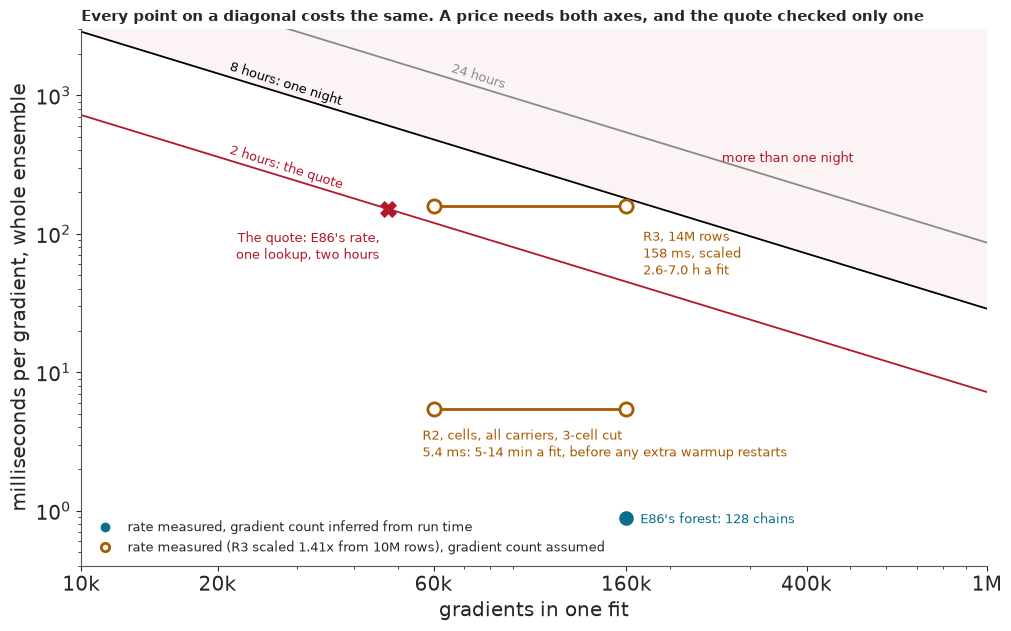
The contractor's rate is right by accident. E86's rate per lookup is about 5x slower than this model's (0.34 against 0.07 ns per chain and lookup), but the sum counts one lookup a row where R3 has five, and the two errors cancel: 151 ms against 158 ms a gradient. What the quote is missing is the other two factors. At 158 ms a gradient, two hours buys at most about 46,000 gradients. At 60,000 the quote misses by 1.3x and one fit takes 2.6 hours; at 160,000 it takes 7.0. A test on three months costs 5.9-16 hours with all earlier rows, or 3.9-10.5 hours on a 12-month window. All of these are extrapolated from one measured gradient at 10M rows, and the gradient counts are assumptions.
On the map, each diagonal is one budget: every point on it costs the same. The hollow orange points use measured rates and assumed gradient counts, and R3's rate is also scaled from 10M rows. The blue dot is E86's measured rate at a count inferred from its run time. The quote is exposed by moving right along a flat line: its rate is fine, but it meets two hours only left of 60,000 gradients.
Neither count is solid. The only measured count in this notebook comes from part 6, where nutpie spends about 60,000 gradients a chain on about 5,000 parameters: a hint from a different sampler, not a measurement of R3. 160,000 is E86's whole run, inferred from its time, on a forest with 24,810 parameters, and only 27,161 of those gradients were sampling; it includes E86's own warmup restart, and any further restart would add to it. R3 has about 747,000 parameters. Nor is 160,000 a ceiling. E86 ran 128 chains and the price uses 32; matching E86's effective sample size with a quarter of the chains needs about four times its sampling gradients, about 240,000 in all, or 10.6 hours, which is more than a night.
R2 sits far below R3 on the map, for two reasons. On the same 12 months, rows would cost about 79 ms a gradient and R2's cells cost 5.4 ms, so collapsing rows into flight x month cells is worth about 15x a gradient, with no hardware bought. The rest of the 29x gap between the two lines comes from setting 24 months of rows against 12 months of cells: from dropping half the data, not from collapsing it.
2 · The flights
The table comes from 24 monthly BTS files, which cover carriers with at least 0.5% of domestic scheduled passenger revenue, so smaller regional operators are absent. Each flight x month cell holds a count of operations and of late or cancelled arrivals, and a cell with 10 or more operations is eligible. We forecast three held-out months, April, July and October 2025, each from the 12 months before it, and treat the target month's operations as known. A real list would have to guess next month's schedule; part 5 shows what that costs. Results are never pooled across months, for a reason the chart makes plain.
data.describe("e87_flights")
data.describe("e87_month_rows")
archive = np.load(data.path("e87_flights"))
flight_carrier, flight_origin, flight_dest = archive["flight_carrier"], archive["flight_origin"], archive["flight_dest"]
cells = pd.DataFrame({"flight": archive["cell_flight"], "month": archive["cell_month"].astype(int),
                      "n": archive["cell_n"].astype(int), "late": archive["cell_late"].astype(int)})
cells["rate"] = cells["late"] / cells["n"]
cells["flagged"] = cells["rate"] > 0.5
cells["carrier"] = flight_carrier[cells["flight"]]
same = (cells["flight"].to_numpy()[1:] == cells["flight"].to_numpy()[:-1]) & (
    cells["month"].to_numpy()[1:] == cells["month"].to_numpy()[:-1] + 1)
cells["state"] = np.r_[-1, np.where(same, cells["flagged"].to_numpy()[:-1].astype(int), -1)]  # last month: 1, 0, or not eligible
cells["last_rate"] = np.r_[np.nan, np.where(same, cells["rate"].to_numpy()[:-1], np.nan)]
print(f"{summary['rows']:,} rows in 24 monthly files, {summary['flight_months']:,} flight x month cells, "
      f"{summary['rows_per_cell']:.1f} rows a cell.")
print(f"Here: {len(cells):,} eligible cells (10 or more operations), {len(flight_carrier):,} flights, "
      f"{cells['flagged'].sum():,} flagged. Late or cancelled: {summary['late_share']:.1%} of rows.")
print(f"Diverted rows not counted late: {summary['diverted_not_late']:,}. "
      f"Target flights with no history: " + ", ".join(
          f"{TARGET_NAMES[t]} {1 - v['target_flights_with_history'] / v['target_flights']:.0%}"
          for t, v in zip(TARGETS, summary["linking"]["training_windows"].values())))

labels = pd.period_range("2024-01", periods=24, freq="M").astype(str)
fig, ax = plt.subplots(figsize=(11, 4.2), layout="constrained")
bar_colour = [ALARM if m in TARGETS else "#9db9c7" for m in by_month["month"]]
ax.bar(by_month["month"], by_month["flagged"], color=bar_colour, width=0.82)
ax.axhline(50, color="k", lw=0.9, ls=":")
ax.annotate("the list has 50 places", (9, 50), xytext=(0, 4), textcoords="offset points", ha="center", fontsize=9)
for m, flagged in zip(by_month["month"], by_month["flagged"]):
    ax.annotate(f"{flagged:,}", (m, flagged), xytext=(0, 3), textcoords="offset points", ha="center", fontsize=7.5,
                color=ALARM if m in TARGETS else "#4a4a4a")
ax.set(yscale="log", ylim=(15, 3500), ylabel="flights flagged that month", xticks=by_month["month"][::3])
ax.set_xticklabels(labels[::3])
ax.legend(handles=[Patch(color=ALARM, label="the three held-out targets"), Patch(color="#9db9c7", label="other months")],
          loc="upper left", ncols=2)
ax.set_title("Flags swing about 67-fold between months, so one good list proves little", loc="left", fontsize=11);
e87_flights: NumPy archive, not a table: open data.path() with np.load. One row per eligible flight x month cell, 494,547 in all: cell_flight, cell_month (0 is 2024-01), cell_n (operations, 10 or more), cell_late (more than 30 minutes late at arrival, or cancelled). One row per flight, 128,423: flight_carrier, flight_origin, flight_dest (most-used airports). A flight is a cluster of departures in the sense of 14 CFR 399.81(c), linked across months as the build script describes, not an official flight. Carrier, airport and flight codes are shuffled integers, with no labels, scheduled times or flight numbers. That removes names, not identity: anyone with the public files can match the codes back. `notice` holds the source notice.
  source: US DOT Bureau of Transportation Statistics, TranStats, Reporting Carrier On-Time Performance (1987-present), the 24 monthly files of 2024-2025. No licence or terms were found for this table, so only re-coded tables are kept, one of them row-level for one month. DERIVED by tools/build_e87_data.py --tables - keep the cached file. No endorsement by BTS or DOT is implied.
  url:    https://transtats.bts.gov/DatabaseInfo.asp?QO_VQ=EFD
e87_month_rows: NumPy archive, not a table: open data.path() with np.load. 547,271 rows in the file's own order, so anyone with the public file can match the codes back: y (late or cancelled), day, carrier, origin, dest, flight, tail, as integers with no names. Flight and tail codes run by first appearance in the file. Tail 0 and any other tail code are not aircraft registrations; rows with no tail share one code. `notice` holds the source notice.
  source: As `e87_flights`: one month, 2024-01. DERIVED by tools/build_e87_data.py --tables - keep the cached file. No endorsement by BTS or DOT is implied.
  url:    https://transtats.bts.gov/DatabaseInfo.asp?QO_VQ=EFD
14,080,680 rows in 24 monthly files, 921,766 flight x month cells, 15.3 rows a cell.
Here: 494,547 eligible cells (10 or more operations), 128,423 flights, 9,711 flagged. Late or cancelled: 15.1% of rows.
Diverted rows not counted late: 36,757. Target flights with no history: 2025-04 22%, 2025-07 11%, 2025-10 25%
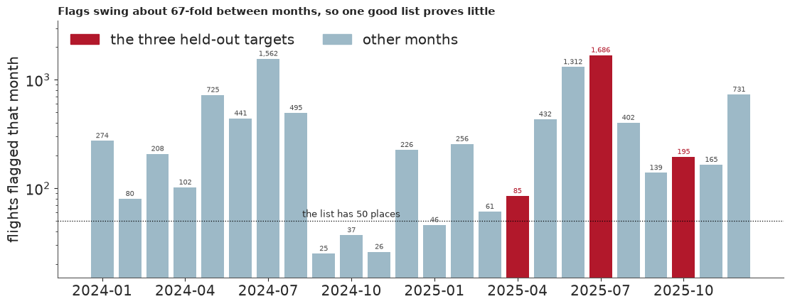
Fourteen million rows collapse to 921,766 flight x month cells, about 15 rows each, and 494,547 of them are eligible. 15% of operations were late or cancelled, and 9,711 eligible cells were flagged. Flags swing about 67-fold between months, from 25 to 1,686, and two things follow. Four months had fewer flags than the list has places, so in a calm month even a perfect list of 50 would hold flights nobody flagged. And the three test months differ 20-fold, so a precision from one of them says little about another.
These flights are short-lived as we link them. Over all 259,558 linked flights, eligible or not, the median one lasts 2 months, and part of that is our linking, which splits some real flights: 28% of new eligible flights had the same number in the same market the month before. In April and October 22-25% of the target flights have no history at all, and 11% in July. Any list here is partly a list of new flights.
3 · What a gradient costs
A rate measured on one model is a rate for its cost shape: the mix of dense algebra, special functions, sequential steps and memory traffic in its gradient. We time five shapes:
- E86's forest: dense matrix products on a lattice;
- a negative binomial on 17,379 hourly bike hires: a design matrix and three
gammalna row; - stochastic volatility on 5,000 daily returns: a recursion through
jax.lax.scan; - R2's likelihood on every carrier's cells: six
gammalna cell, with a flight effect only for flights seen in 3 or more cells (part 4 says why); - R3 on one month of rows: five lookups a row, whose reverse pass is a scatter-add.
E86 had no lookups at all, which is why its rate might not transfer. First, the index pattern of a month of rows; each panel has one point per row.
month = np.load(data.path("e87_month_rows"))
day = month["day"].astype(np.int64)
columns = {"carrier": month["carrier"].astype(np.int64), "flight": month["flight"].astype(np.int64),
           "origin_day": month["origin"] * 32 + day, "dest_day": month["dest"] * 32 + day,
           "tail": month["tail"].astype(np.int64)}
outcome = month["y"]
n_month = outcome.size
by_flight = np.argsort(columns["flight"], kind="stable")
adjacent = (columns["flight"][1:] == columns["flight"][:-1]).mean()
print(f"Adjacent rows share a flight {adjacent:.0%} of the time, and a tail "
      f"{(columns['tail'][1:] == columns['tail'][:-1]).mean():.0%}")

fig, axes = plt.subplots(1, 2, figsize=(11, 4.4), sharey=True, layout="constrained")
for ax, order, title in zip(axes, (np.arange(n_month), by_flight), ("Rows as the file holds them", "Rows sorted by flight")):
    art = ax.hexbin(np.arange(n_month) / 1e3, columns["flight"][order] / 1e3, gridsize=70, cmap="viridis", norm=LogNorm(1, 3000),
                    mincnt=1, linewidths=0)
    ax.set(title=title, xlabel="row, thousands")
axes[0].set_ylabel("flight code, thousands")
fig.colorbar(art, ax=axes, shrink=0.85, label="rows in a hexagon");
Adjacent rows share a flight 35% of the time, and a tail 6%
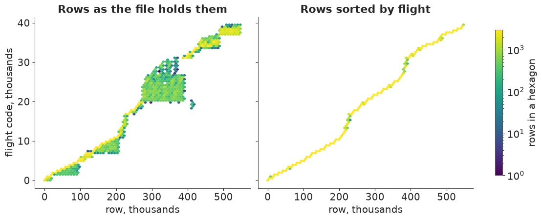
The file visits flights in blocks and returns to them day after day: adjacent rows share a flight 35% of the time and a tail only 6%. Sorting by flight puts a flight's rows side by side, which should make the scatter-add of the reverse pass cheaper. We test that in a moment.
Now the timing. time_gradient waits for the result, takes the best of three calls, and checks that
every output is finite. Rows are timed on this machine's CPU in this run, at 1 and 8 chains on 2
threads; the GPU column is loaded from the stored tables.
def field_model():
    """Row 1: E86's four-field forest at 20 m, as a flat JAX log density. A PyMC model, priced as it stands."""
    data.describe("bei_trees")
    raw = np.load(data.path("bei_trees"))
    cell, m_fine, m_smooth, half = 20.0, (25, 50), (20, 20), 800.0
    nx, ny = int(1000 / cell), int(500 / cell)
    y = np.histogram2d(raw["y"], raw["x"], bins=[ny, nx], range=[[0, 500], [0, 1000]])[0]
    k = int(cell / 5)

    def to_cells(v):
        c = 0.25 * (v[:-1, :-1] + v[1:, :-1] + v[:-1, 1:] + v[1:, 1:])
        c = c.reshape(ny, k, nx, k).mean((1, 3))
        return ((c - c.mean()) / c.std()).astype("float32")

    def basis(n, half_width, m):
        x = (np.arange(n) + 0.5) * cell
        x = x - x.mean()
        w = np.pi * np.arange(1, m + 1) / (2 * half_width)
        return (np.sqrt(1 / half_width) * np.sin(w[None, :] * (x[:, None] + half_width))).astype("float32"), w

    def density(w2, ell, nu):
        constant = {0.5: 2 * np.pi / ell, 1.5: 6 * np.pi * 3**1.5 / ell**3}[nu]
        return pt.sqrt(constant) * ((2 * nu) / ell**2 + w2) ** (-(nu + 1) / 2)

    elev, grad = to_cells(raw["elev"]), to_cells(np.log(raw["grad"]))
    Py, wy = basis(ny, 312.5, m_fine[0])
    Px, wx = basis(nx, 625.0, m_fine[1])
    Qy, vy = basis(ny, half, m_smooth[0])
    Qx, vx = basis(nx, half, m_smooth[1])
    w2 = (wy[:, None] ** 2 + wx[None, :] ** 2).astype("float32")
    v2 = (vy[:, None] ** 2 + vx[None, :] ** 2).astype("float32")
    pytensor.config.floatX = "float32"
    try:
        with pm.Model() as model:
            alpha = pm.Normal("alpha", np.log(30.0), 1.0)
            b_elev, b_grad = pm.Normal("b_elev", 0.0, 1.0), pm.Normal("b_grad", 0.0, 1.0)
            s_broad = pm.LogNormal("s_broad", np.log(0.7), 0.5)
            ell_broad = pm.LogNormal("ell_broad", np.log(120.0), 0.4)
            s_fine = pm.LogNormal("s_fine", np.log(0.7), 0.5)
            ell_fine = pm.LogNormal("ell_fine", np.log(20.0), 0.6)
            s_slope_elev = pm.LogNormal("s_slope_elev", np.log(0.5), 0.5)
            s_slope_grad = pm.LogNormal("s_slope_grad", np.log(0.5), 0.5)
            ell_slope = pm.LogNormal("ell_slope", np.log(200.0), 0.4)
            z_broad = pm.Normal("z_broad", 0.0, 1.0, shape=m_smooth)
            z_fine = pm.Normal("z_fine", 0.0, 1.0, shape=m_fine)
            z_elev = pm.Normal("z_elev", 0.0, 1.0, shape=m_smooth)
            z_grad = pm.Normal("z_grad", 0.0, 1.0, shape=m_smooth)
            smooth = lambda z, sd: Qy @ (sd * z) @ Qx.T
            sd_slope = density(v2, ell_slope, 1.5)
            eta = (alpha + (b_elev + smooth(z_elev, s_slope_elev * sd_slope)) * elev
                   + (b_grad + smooth(z_grad, s_slope_grad * sd_slope)) * grad
                   + smooth(z_broad, s_broad * density(v2, ell_broad, 1.5))
                   + Py @ (s_fine * density(w2, ell_fine, 0.5) * z_fine) @ Px.T + np.log(cell**2 / 1e4))
            pm.Poisson("y", pt.exp(eta), observed=y)
        logp = get_jaxified_logp(model)
        start = model.initial_point()
        q0, unravel = ravel_pytree([jnp.asarray(start[v.name]) for v in model.value_vars])
    finally:
        pytensor.config.floatX = "float64"
    return (lambda q: logp(unravel(q))), q0, y.size


def negative_binomial():
    """Row 2: bike hours, a design matrix and three gammaln a row."""
    data.describe("bike_hour")
    bike = data.load("bike_hour")
    X = pd.get_dummies(bike[["hr", "weekday", "mnth", "weathersit"]].astype(str), drop_first=True, dtype=float)
    X = np.c_[np.ones(len(X)), X.to_numpy(), bike[["temp", "hum", "windspeed"]].to_numpy(float)].astype(np.float32)
    counts, design = jnp.asarray(bike["cnt"].to_numpy(float), jnp.float32), jnp.asarray(X)

    def f(q):
        log_alpha, beta = q[0], q[1:]
        mu, alpha = jnp.exp(design @ beta), jnp.exp(log_alpha)
        lp = (jax_gammaln(counts + alpha) - jax_gammaln(alpha) - jax_gammaln(counts + 1)
              + alpha * (log_alpha - jnp.log(alpha + mu)) + counts * (jnp.log(mu) - jnp.log(alpha + mu)))
        return jnp.sum(lp) - 0.5 * jnp.sum(q * q) / 25.0

    return f, jnp.zeros(X.shape[1] + 1, jnp.float32).at[1].set(4.0), X.shape[0]


def stochastic_volatility():
    """Row 3: one industry's last 5,000 daily returns, a recursion through `jax.lax.scan`."""
    data.describe("ff_industries12_daily")
    ff = data.load("ff_industries12_daily").iloc[:, :12].apply(pd.to_numeric, errors="coerce")
    ff = ff.loc[[str(i).strip().isdigit() for i in ff.index]]
    r = ff.iloc[:, 0].to_numpy(float)
    r = r[(r > -99) & np.isfinite(r)][-5000:]
    returns = jnp.asarray(r / r.std(), jnp.float32)

    def f(q):
        mu, log_s, raw_phi, z = q[0], q[1], q[2], q[3:]
        s, phi = jnp.exp(log_s), jnp.tanh(raw_phi)

        def step(h, zt):
            h = mu + phi * (h - mu) + s * zt
            return h, h

        _, h = jax.lax.scan(step, mu, z)
        lp = -0.5 * (h + returns**2 * jnp.exp(-h))
        return jnp.sum(lp) - 0.5 * jnp.sum(z * z) - 0.5 * (mu**2 + log_s**2 + raw_phi**2)

    return f, jnp.zeros(returns.size + 3, jnp.float32).at[2].set(2.0), returns.size


def cell_model(target=TARGETS[0]):
    """Row 4: R2 on every carrier's cells, with a flight effect only for flights of 3 or more cells."""
    w = cells[(cells["month"] >= target - WINDOW) & (cells["month"] < target)]
    counts = np.bincount(w["flight"], minlength=flight_carrier.size)
    kept = np.flatnonzero(counts >= 3)
    own = counts[w["flight"]] >= 3
    code = np.where(own, np.searchsorted(kept, w["flight"]), kept.size)  # the last level is held at 0
    look = [np.unique(flight_carrier[w["flight"]], return_inverse=True)[1], np.unique(flight_origin[w["flight"]], return_inverse=True)[1],
            np.unique(flight_dest[w["flight"]], return_inverse=True)[1], w["month"].to_numpy() - (target - WINDOW)]
    sizes = [int(i.max()) + 1 for i in look] + [kept.size]
    cuts = np.cumsum(sizes)[:-1]
    look = [jnp.asarray(i, jnp.int32) for i in look + [code]]
    n, k = jnp.asarray(w["n"].to_numpy(), jnp.float32), jnp.asarray(w["late"].to_numpy(), jnp.float32)

    def f(q):
        log_phi, rest = q[0], q[1:]
        parts = jnp.split(rest, cuts)
        parts[-1] = jnp.concatenate([parts[-1], jnp.zeros(1, q.dtype)])
        eta = sum(p[i] for p, i in zip(parts, look))
        phi, p = jnp.exp(log_phi), jax.nn.sigmoid(eta)
        a, b = p * phi, (1 - p) * phi
        lp = (jax_gammaln(k + a) + jax_gammaln(n - k + b) - jax_gammaln(n + a + b)
              + jax_gammaln(a + b) - jax_gammaln(a) - jax_gammaln(b))
        return jnp.sum(lp) - 0.5 * jnp.sum(rest * rest) - 0.5 * log_phi * log_phi

    return f, jnp.zeros(sum(sizes) + 1, jnp.float32).at[0].set(3.0), len(w)


def row_model(rows):
    """Row 5: Bernoulli-logit with five lookups, on these rows. Codes are remade, so d follows the rows."""
    codes = [np.unique(columns[k][rows], return_inverse=True)[1] for k in columns]
    sizes = [int(c.max()) + 1 for c in codes]
    cuts = np.cumsum(sizes)[:-1]
    look = [jnp.asarray(c, jnp.int32) for c in codes]
    y = jnp.asarray(outcome[rows], jnp.float32)

    def f(q):
        eta = sum(p[i] for p, i in zip(jnp.split(q, cuts), look))
        return jnp.sum(y * eta - jnp.logaddexp(0.0, eta)) - 0.5 * jnp.sum(q * q)

    return f, jnp.zeros(sum(sizes), jnp.float32), rows.size


def timed(row, f, q0, size, chains=(1, 8)):
    rows = time_gradient(f, q0, chains=chains, repeat=3, seed=87)
    assert all(r["finite"] for r in rows), row
    return {"row": row, "size": size, "d": int(q0.size), **{f"cpu_{r['chains']}": r["run_ms"] for r in rows}}


with stage("timing rows 1-5"):
    table = [timed("1 forest, dense products", *field_model()), timed("2 bikes, gammaln", *negative_binomial()),
             timed("3 volatility, scan", *stochastic_volatility()), timed("4 cells, R2 likelihood", *cell_model()),
             timed("5 rows, five lookups", *row_model(np.arange(n_month)))]
rows_cpu = pd.DataFrame(table).set_index("row")
best = lambda job: {r["chains"]: r["run_ms"] for r in job["rows"]}
gpu_8 = {"1 forest, dense products": (min(best(jobs["p1_a"])[8], best(jobs["p1_b"])[8]), 20_000, 8),
         "2 bikes, gammaln": (best(extra_gpu["row2"])[8], 17_379, 8),
         "3 volatility, scan": (best(extra_gpu["row3"])[8], 5_000, 8),
         "4 cells, R2 likelihood": (r2_gpu_ms, jobs["r2_gpu"]["shape"]["cells"], CHAINS),
         "5 rows, five lookups": (extra_gpu["row5_month"]["month_file"][0]["run_ms"], n_month, 8)}
rows_cpu["cpu ns/chain-row"] = rows_cpu["cpu_8"] * 1e6 / (8 * rows_cpu["size"])
rows_cpu["gpu ms"] = [v[0] for v in gpu_8.values()]
rows_cpu["gpu ns/chain-row"] = [v[0] * 1e6 / (v[1] * v[2]) for v in gpu_8.values()]
rows_cpu["cpu / gpu"] = rows_cpu["cpu ns/chain-row"] / rows_cpu["gpu ns/chain-row"]
print(rows_cpu.round(3).to_string())
print("Not matched: GPU row 1 is the 5 m lattice of 20,000 cells against 1,250 on the CPU, and GPU row 4 is 32 chains against "
      "8. Rows 2, 3 and 5 are 8 chains on the same problem.")
print("GPU row 3 by chains (ms):", {k: round(v, 1) for k, v in best(extra_gpu["row3"]).items()})
row3_128 = best(extra_gpu["row3"])[128] * 1e6 / (128 * 5_000)
print(f"Row 3 at 128 chains costs {row3_128:.0f} ns per chain-row on the card, "
      f"{row3_128 / rows_cpu.loc['3 volatility, scan', 'cpu ns/chain-row']:.0f}x the CPU's 8-chain rate.")
month_by_chains = {r["chains"]: r["run_ms"] for r in extra_gpu["row5_month"]["month_file"]}
chain_saving = (month_by_chains[8] / 8) / (month_by_chains[32] / 32)
print(f"Row 5 on the card: cost per chain falls {chain_saving:.2f}x from 8 to 32 chains, so row 4's ratio is flattered "
      f"by about that much: about {rows_cpu.loc['4 cells, R2 likelihood', 'cpu / gpu'] / chain_saving:.0f}x if row 4 behaves like row 5.")

fig, ax = plt.subplots(figsize=(10, 3.8), layout="constrained")
order = rows_cpu.index[::-1]
UNMATCHED = {"1 forest, dense products": "1 forest, dense products\n(not matched: GPU 20,000 cells, CPU 1,250)",
             "4 cells, R2 likelihood": "4 cells, R2 likelihood\n(not matched: GPU 32 chains, CPU 8)"}
for i, row in enumerate(order):
    c, g = rows_cpu.loc[row, ["cpu ns/chain-row", "gpu ns/chain-row"]]
    ax.plot([c, g], [i, i], color=ALARM if g > c else "#b9c6cd", lw=4, solid_capstyle="round", zorder=1)
    ax.annotate(f"GPU {c / g:.0f}x cheaper" if c > g else f"GPU {g / c:.0f}x dearer", (max(c, g), i), xytext=(10, 0),
                textcoords="offset points", va="center", fontsize=9, color=ALARM if g > c else "#33424b")
ax.scatter(rows_cpu.loc[order, "cpu ns/chain-row"], range(5), s=70, marker="o", color=CALM, zorder=2, label="CPU, 2 threads, 8 chains")
ax.scatter(rows_cpu.loc[order, "gpu ns/chain-row"], range(5), s=70, marker="s", color=MEASURED, zorder=2, label="GPU, stored table")
ax.set(xscale="log", yticks=range(5), xlim=(0.04, 4000), xlabel="nanoseconds per chain and row, measured")
ax.set_yticklabels([UNMATCHED.get(row, row) for row in order])
ax.legend(loc="upper left", bbox_to_anchor=(1.01, 1), fontsize=9)
ax.set_title("A rate belongs to a cost shape: the same card wins four rows and loses one by a wide margin", loc="left", fontsize=11);
bei_trees: Exact positions (x, y in metres) of the Beilschmiedia pendula trees in the 1000 x 500 m plot, with elevation (elev, m) and its gradient norm (grad) on a 5 m grid (yrow x xcol). Not a table: open data.path() with np.load.
  source: Hubbell & Foster (1983), Condit, Hubbell & Foster (1996) and Condit (1998), Barro Colorado Island forest dynamics plot, Panama; as shipped with the R package `spatstat.data` 3.1-9 (GPL >= 2), analysed by Moller & Waagepetersen (2007). CONVERTED from the R file by tools/build_e86_bei.py - keep the cached file.
  url:    https://raw.githubusercontent.com/cran/spatstat.data/master/data/bei.rda
bike_hour: Hourly rental counts 2011-2012 with weather and calendar covariates.
  source: Fanaee-T & Gama (2013), Capital Bikeshare (Washington DC), UCI ML Repository.
  url:    https://archive.ics.uci.edu/static/public/275/bike+sharing+dataset.zip
ff_industries12_daily: Daily % returns of 12 US industry portfolios since July 1926 (NoDur ... Other). The file holds TWO blocks, value-weighted then equal-weighted, each headed by a text line: keep the rows before the first non-date index. -99.99 marks missing.
  source: Kenneth R. French Data Library (Fama & French, CRSP), 12 industry portfolios; updated monthly.
  url:    https://mba.tuck.dartmouth.edu/pages/faculty/ken.french/ftp/12_Industry_Portfolios_daily_CSV.zip
                            size      d   cpu_1    cpu_8  cpu ns/chain-row  gpu ms  gpu ns/chain-row  cpu / gpu
row
1 forest, dense products    1250   2460   0.095    0.413            41.266   0.216             1.348     30.602
2 bikes, gammaln           17379     48   0.636    3.849            27.681   0.127             0.911     30.380
3 volatility, scan          5000   5003   0.138    0.311             7.776  62.820          1570.493      0.005
4 cells, R2 likelihood    246528  31503  32.845  284.673           144.341   5.403             0.685    210.771
5 rows, five lookups      547271  65218  11.304   96.099            21.949   2.724             0.622     35.278
Not matched: GPU row 1 is the 5 m lattice of 20,000 cells against 1,250 on the CPU, and GPU row 4 is 32 chains against 8. Rows 2, 3 and 5 are 8 chains on the same problem.
GPU row 3 by chains (ms): {8: 62.8, 32: 62.6, 128: 62.9}
Row 3 at 128 chains costs 98 ns per chain-row on the card, 13x the CPU's 8-chain rate.
Row 5 on the card: cost per chain falls 1.76x from 8 to 32 chains, so row 4's ratio is flattered by about that much: about 120x if row 4 behaves like row 5.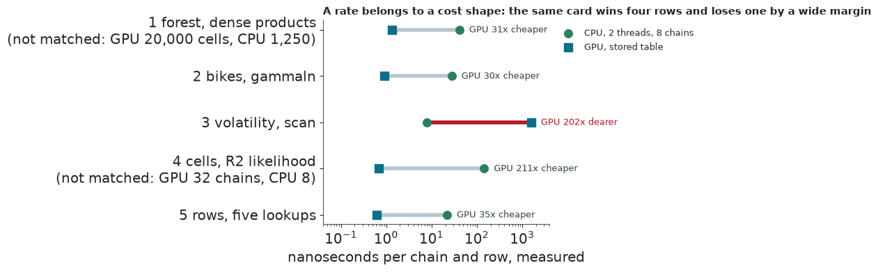
A rate belongs to a cost shape. On four of the five rows the card costs far less per chain and row than 2 CPU threads, but not every ratio is like for like. Rows 2 and 5 are matched, at about 30-35x in this run. Row 1 sets the 5 m lattice of 20,000 cells on the card against 1,250 cells on the CPU. Row 4 sets 32 GPU chains against 8 CPU chains, and row 5 shows the card's cost per chain falling 1.76x between those counts, so row 4's 210x is flattered: about 120x if it behaves like row 5.
Row 3, the scan, goes the other way. At 8 chains the card costs about 200x more than the CPU,
and its time hardly moves with the number of chains: 63 ms at 8, 32 and 128. A recursion runs one
step at a time on the card, however many chains share it. The gap shrinks as chains are added, to
about 13x at 128 chains against the CPU's 8-chain rate, but no single rate prices all five rows. On
the CPU, row 4 is the dearest at about 144 ns a chain and cell; its six gammaln are the likely
reason, though they were not timed alone.
The CPU side is 2 threads, so the table shows where the time goes, not that a GPU beats a well-run CPU.
Failure 1: sorting the rows
We expected the reverse pass of a lookup, a scatter-add into scattered places, to be the slow part, and planned to fix it by sorting the rows by flight. The next cell climbs from one day of rows to the whole month, in file order and sorted, at 1 and 8 chains, and fits a power law to the small sizes to predict the month. The right panel loads a different test from the card: one lookup at 10 million rows, in file order, sorted, and sorted with JAX told that the indices are sorted.
def run_ladder(days=(1, 3, 7, 14, 31)):
    """Row 5 on the first `d` days of the month, in file order and sorted by flight, at 1 and 8 chains."""
    out = []
    for last in days:
        rows = np.flatnonzero(day <= last)
        for name, used in (("file", rows), ("sorted", rows[np.argsort(columns["flight"][rows], kind="stable")])):
            f, q0, size = row_model(used)
            for r in time_gradient(f, q0, chains=(1, 8), repeat=3, seed=87):
                out.append({"days": last, "order": name, "chains": r["chains"], "rows": size, "d": int(q0.size), "ms": r["run_ms"]})
    return pd.DataFrame(out)


with stage("row 5 ladder"):
    ladder = run_ladder()
print(ladder.pivot_table(index=["days", "rows"], columns=["order", "chains"], values="ms").round(2).to_string())


def predict_month(fit_days=(1, 3, 7), chains=8, order="file"):
    """Fit a power law on small subsets, and predict the whole month's time."""
    part = ladder[(ladder["chains"] == chains) & (ladder["order"] == order)].set_index("days")
    slope, level = np.polyfit(np.log(part.loc[list(fit_days), "rows"]), np.log(part.loc[list(fit_days), "ms"]), 1)
    predicted = np.exp(level + slope * np.log(part.loc[31, "rows"]))
    return {"slope": slope, "predicted_ms": predicted, "measured_ms": part.loc[31, "ms"],
            "error": predicted / part.loc[31, "ms"] - 1}


print("Power law from 1, 3 and 7 days:", {k: round(v, 2) for k, v in predict_month().items()})
print("Same, sorted:                  ", {k: round(v, 2) for k, v in predict_month(order="sorted").items()})
print("From 1 and 3 days only:        ", {k: round(v, 2) for k, v in predict_month(fit_days=(1, 3)).items()})
week = ladder[(ladder["days"] == 7) & (ladder["order"] == "file") & (ladder["chains"] == 8)].iloc[0]
whole = ladder[(ladder["days"] == 31) & (ladder["order"] == "file") & (ladder["chains"] == 8)].iloc[0]
print(f"Straight line from the week alone: {week['ms'] * whole['rows'] / week['rows']:.1f} ms against {whole['ms']:.1f} ms measured")

p3 = {name: jobs[f"p3_{key}"]["10m"] for name, key in (("file", "unsorted_default"), ("sorted", "sorted_nohint_default"),
                                                      ("hint", "sorted_hint_default"))}
fig, axes = plt.subplots(1, 2, figsize=(12, 4.6), layout="constrained", width_ratios=(1.1, 1))
ax = axes[0]
for (name, chains), part in ladder.groupby(["order", "chains"]):
    ax.plot(part["rows"], part["ms"], "o-" if name == "file" else "s--", color=MEASURED if chains == 8 else CALM, lw=1.2, ms=5,
            label=f"{name} order, {chains} chain{'s' if chains > 1 else ''}")
ax.set(xscale="log", yscale="log", xlabel="rows", ylabel="ms per gradient")
ax.set_title("CPU, 2 threads, a month of rows, measured", fontsize=10.5, loc="left")
ax.xaxis.set_major_formatter(FuncFormatter(lambda v, _: f"{v / 1e3:.0f}k"))
ax.xaxis.set_minor_formatter(NullFormatter())
ax.set_xticks(sorted(ladder["rows"].unique()))
ax.legend(fontsize=8.5)
ax = axes[1]
steps = [("File order", p3["file"]["run_ms"], "total"),
         ("forward", p3["sorted"]["forward_ms"] - p3["file"]["forward_ms"], "step"),
         ("reverse", p3["sorted"]["reverse_extra_ms"] - p3["file"]["reverse_extra_ms"], "step"),
         ("Sorted", p3["sorted"]["run_ms"], "total"),
         ("hint,\nreverse", p3["hint"]["reverse_extra_ms"] - p3["sorted"]["reverse_extra_ms"], "step"),
         ("Sorted\n+ hint", p3["hint"]["run_ms"], "total")]
level = 0.0
for i, (label, value, kind) in enumerate(steps):
    if kind == "total":
        ax.bar(i, value, color=MEASURED, width=0.66)
        level = value
        ax.annotate(f"{value:.2f}", (i, value), xytext=(0, 3), textcoords="offset points", ha="center", fontsize=9)
    else:
        ax.bar(i, value, bottom=level, color=ALARM if value > 0 else CALM, width=0.66)
        level += value
        ax.annotate(f"{value:+.2f}", (i, max(level, level - value)), xytext=(0, 3), textcoords="offset points", ha="center", fontsize=9)
ax.set_xticks(range(len(steps)), [s[0] for s in steps], fontsize=9)
ax.set(ylabel="ms per gradient")
ax.set_title("GPU, one lookup on 10M rows and its reverse, 8 chains, measured", fontsize=10.5, loc="left")
fig.suptitle("Sorting by flight was the planned fix. It costs time on the GPU, and hardly matters on a month", x=0.01, ha="left", fontsize=11);
order         file        sorted
chains           1      8      1       8
days rows
1    17265    0.32   1.61   0.31    1.64
3    54762    0.70   3.98   0.68    3.63
7    126699   2.71  21.81   2.65   20.70
14   248897   5.17  44.42   5.10   40.24
31   547271  11.36  97.51  11.32  100.66
Power law from 1, 3 and 7 days: {'slope': np.float64(1.28), 'predicted_ms': np.float64(111.81), 'measured_ms': np.float64(97.51), 'error': np.float64(0.15)}
Same, sorted:                   {'slope': np.float64(1.24), 'predicted_ms': np.float64(97.86), 'measured_ms': np.float64(100.66), 'error': np.float64(-0.03)}
From 1 and 3 days only:         {'slope': np.float64(0.78), 'predicted_ms': np.float64(24.17), 'measured_ms': np.float64(97.51), 'error': np.float64(-0.75)}
Straight line from the week alone: 94.2 ms against 97.5 ms measured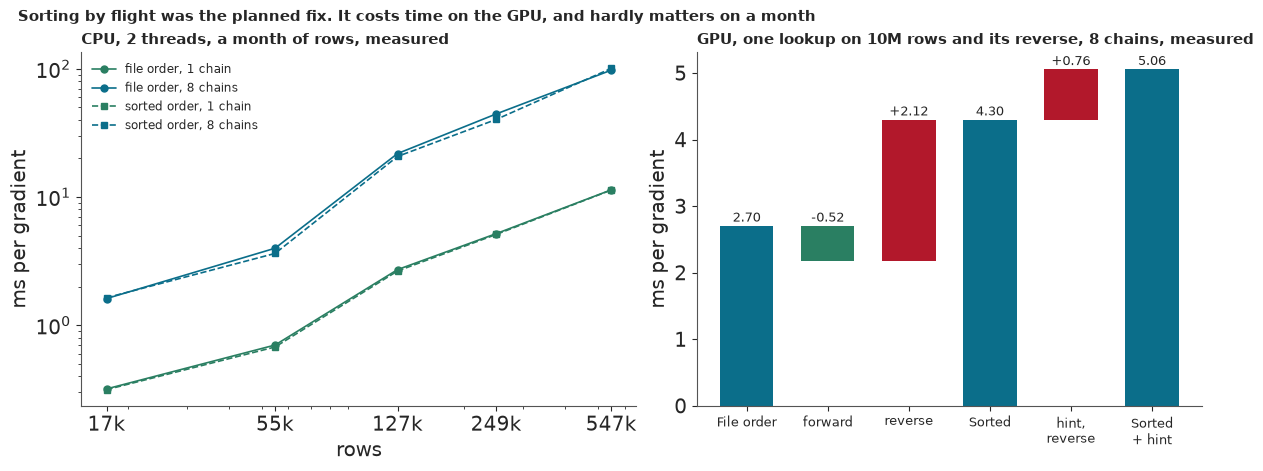
The slow scatter did not appear, and the fix made things worse. On the card, sorting cuts the forward pass by 0.52 ms but adds 2.12 ms to the reverse pass, so a gradient goes from 2.70 to 4.30 ms, and telling JAX the indices are sorted adds another 0.76 ms: 1.6-1.9x slower in all. On a month of rows with five lookups, sorting changes nothing, on the card (2.7 ms either way at 8 chains) or on the CPU. We did not find the cause, and because size and the number of lookups changed together between the two tests, we cannot say which matters; the gradients are still exact. The lesson we expected was "collapse, then sort, then buy". The one the data give is shorter: collapse first, then measure.
A cost law needs a warning too. On the CPU, going from 3 days to 7 multiplies the rows by 2.3 and the time by 4-6, at 1 chain and at 8, and the step repeats from run to run. Part of the step is threading, since one pinned core removes it at 1 chain, so the CPU column of row 5 is not a clean 2-core rate. A power law fitted on 1, 3 and 7 days lands within about 15% of the month only by luck, because it straddles the step; fitted on 1 and 3 days alone it misses the month by three quarters. Small subsets are cheap to time, and they can sit on the wrong side of a step.
On the card, 500k and 10M rows ran at 0.074 and 0.070 ns per chain and lookup, so the last step from 10M to 14M rows has evidence behind it: two points on one card, which say nothing about any other card.
4 · The walls behind the quote
Time is one wall. Memory and precision are the other two, and neither shows up in a rate.
per_chain_row_gib = cell_10m["vram"]["peak_gb"] / (CHAINS * rows_10m)
grid_rows = np.array([500_089, 1e6, 5e6, 10_000_174, ROWS])
grid_chains = np.array([8, 16, 32, 64, 128])
vram = per_chain_row_gib * grid_rows[:, None] * grid_chains[None, :]
scaled_500k = vram[0, 2]
vram[0, 2] = cell_500k["vram"]["peak_gb"]  # the other measured cell: scaling from 10M misses it
LIMIT = jobs["p1_a"]["vram"]["limit_gb"]
print(pd.DataFrame(vram, index=[f"{r / 1e6:.1f}M rows" for r in grid_rows], columns=[f"{c} chains" for c in grid_chains]).round(2).to_string())
print(f"Measured: 500k x 32 = {cell_500k['vram']['peak_gb']:.2f} GiB, 10M x 32 = {cell_10m['vram']['peak_gb']:.2f} GiB. Usable VRAM {LIMIT:.2f} GiB.")
print(f"Scaling from 10M would put 500k x 32 at {scaled_500k:.2f} GiB, {vram[0, 2] / scaled_500k:.1f}x too low. "
      "Both measured cells are at 32 chains.")

window_counts = np.bincount(cells.loc[(cells["month"] >= TARGETS[0] - WINDOW) & (cells["month"] < TARGETS[0]), "flight"])
window_cells = cells[(cells["month"] >= TARGETS[0] - WINDOW) & (cells["month"] < TARGETS[0])]
flights_cut, flights_all = jobs["r2_gpu"]["shape"]["levels"]["flight_cut"], int((window_counts > 0).sum())
d_cut = jobs["r2_gpu"]["shape"]["d"]
d_all = d_cut + flights_all - flights_cut
R3_D = 747_000  # plans/large/E87.md section 12: 481k day cells, 260k flights, 6k tails
print(f"The 3-cell cut keeps {flights_cut:,} of {flights_all:,} flights, and "
      f"{(window_counts[window_cells['flight']] < 3).mean():.0%} of cells lose their flight's own effect.")
print("ChEES warmup's d x d table, GiB:", {name: round(d * d * 4 / 2**30, 1) for name, d in
                                          ((f"R2 cut, d {d_cut:,}", d_cut), (f"R2 every flight, d {d_all:,}", d_all), (f"R3, d {R3_D:,}", R3_D))})
per_row = stats.bernoulli.logpmf(outcome, outcome.mean()).mean()
logp_month, logp_14m = abs(per_row) * n_month, abs(per_row) * ROWS
spacing = lambda x: float(np.spacing(np.float32(x)))
print(f"|logp| at the month's own rate: {logp_month:,.0f}, float32 spacing there {spacing(logp_month):.3f} nats. "
      f"At 14M rows with this month's rate: {logp_14m:,.0f}, spacing {spacing(logp_14m):.2f} nats (arithmetic, not a test).")

fig, axes = plt.subplots(1, 2, figsize=(12, 4.6), layout="constrained", width_ratios=(1.15, 1))
ax = axes[0]
mesh = ax.imshow(vram, cmap="YlGnBu", norm=LogNorm(0.1, 100), origin="lower", aspect="auto")
for i in range(grid_rows.size):
    for j in range(grid_chains.size):
        over = vram[i, j] > LIMIT
        ax.text(j, i, f"{vram[i, j]:.2f}" if (i, j) == (0, 2) else f"{vram[i, j]:.1f}", ha="center", va="center", fontsize=9.5,
                color="w" if vram[i, j] > 10 else "k", weight="bold" if over else None)
        if over:
            ax.add_patch(Rectangle((j - 0.5, i - 0.5), 1, 1, fill=False, hatch="///", edgecolor=ALARM, lw=0))
for i in (0, 3):
    ax.add_patch(Rectangle((1.5, i - 0.5), 1, 1, fill=False, edgecolor=EXTRA, lw=2.5))
ax.set(xticks=range(5), yticks=range(5), xlabel="chains", ylabel="rows, five lookups")
ax.set_xticklabels(grid_chains)
ax.set_yticklabels(["500k", "1M", "5M", "10M", "14M"])
ax.grid(False)
ax.set_title(f"VRAM in GiB. Orange boxes are measured, the rest are scaled.\nHatched cells pass the {LIMIT:.2f} GiB limit", fontsize=10.5, loc="left")
fig.colorbar(mesh, ax=ax, shrink=0.8)
ax = axes[1]
x = np.logspace(3, 8, 600)
ax.step(x, np.spacing(x.astype(np.float32)), where="post", color="k", lw=1.2)
points = [("E86 forest", abs(jobs["p1_a"]["logp_at_start"]), True), ("a month of rows", logp_month, True), ("14M rows", logp_14m, False)]
for name, value, known in points:
    ax.scatter([value], [spacing(value)], s=80, color=MEASURED if known else "w", edgecolor=MEASURED if known else EXTRA, lw=2, zorder=3)
    ax.annotate(name, (value, spacing(value)), xytext=(-8, 8), textcoords="offset points", ha="right", fontsize=9.5)
ax.axhline(1.0, color=ALARM, lw=0.9, ls=":")
ax.annotate("1 nat", (1.3e3, 1.0), xytext=(0, 3), textcoords="offset points", color=ALARM, fontsize=9)
ax.set(xscale="log", yscale="log", xlabel="|log density|", ylabel="float32 spacing, nats")
ax.set_title("A total this large has few digits left", fontsize=10.5, loc="left")
fig.suptitle("Two more limits a rate cannot see", x=0.01, ha="left", fontsize=11);
            8 chains  16 chains  32 chains  64 chains  128 chains
0.5M rows       0.05       0.10       0.35       0.40        0.81
1.0M rows       0.10       0.20       0.40       0.81        1.61
5.0M rows       0.50       1.01       2.02       4.04        8.07
10.0M rows      1.01       2.02       4.04       8.07       16.15
14.1M rows      1.42       2.84       5.68      11.37       22.74
Measured: 500k x 32 = 0.35 GiB, 10M x 32 = 4.04 GiB. Usable VRAM 16.56 GiB.
Scaling from 10M would put 500k x 32 at 0.20 GiB, 1.7x too low. Both measured cells are at 32 chains.
The 3-cell cut keeps 30,789 of 72,386 flights, and 24% of cells lose their flight's own effect.
ChEES warmup's d x d table, GiB: {'R2 cut, d 31,503': 3.7, 'R2 every flight, d 73,100': 19.9, 'R3, d 747,000': 2078.7}
|logp| at the month's own rate: 263,495, float32 spacing there 0.031 nats. At 14M rows with this month's rate: 6,779,439, spacing 0.50 nats (arithmetic, not a test).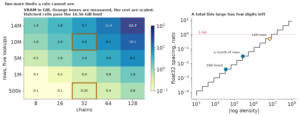
Memory for the gradient is not the wall. Scaled from the measured 10M cell, 32 chains at 14M rows need about 5.7 GiB, and only 128 chains pass the 16.56 GiB this card gives JAX. Only the two orange cells are measured, both at 32 chains. Scaling from the 10M cell misses the other one by 1.7x (0.20 against 0.35 GiB), scaling by chains is untested, and nothing above 10M rows was run, so this wall is arithmetic.
The sampler's own memory is the larger wall, and it sits outside this grid. The grid counts the
gradient only. E86's ChEES recipe, the source of the 160,000 gradients, also keeps a d x d table
during warmup (m2 in blackjax's chees_adaptation). At R3's 747,000 parameters that table is
about 2,080 GiB. It is also why R2 must be cut down before ChEES can run it on all carriers: with an
effect for every flight it has 73,100 parameters and a table of about 20 GiB, over the limit.
Keeping flight effects only for flights seen in 3 or more cells brings it to 31,503 parameters and
3.7 GiB. The price is that only 30,789 of 72,386 flights keep their own effect and 24% of cells
lose it, so the cut model is not the R2 fitted in part 6. A private blackjax option, _length_floor=False,
skips the table; it is untested here, and its gradient count is unknown. So R3's price joins a
gradient count from a recipe that cannot run at this size to a memory figure from one with no count.
Precision is unresolved. At 14 million rows the total log density is near 6.8 million, where neighbouring float32 numbers are 0.5 nats apart; on one month it is about 263,000, with a spacing of 0.03. That is the spacing of the numbers, not the measured error of a real sum, and the check that would measure the error was not run; it cannot be run on a month, where the spacing is small. Rounding of this size changes which proposals are accepted, though it does not by itself cause a divergence. A row-level run must pass this test before anyone relies on its 7.0 hours.
5 · Two counting rules
The analyst's table comes first, because it may win. R0 says a flight flagged last month will be flagged again, with the chance estimated from pairs of consecutive months in the window. R1 adds up each flight's operations and late operations over the 12-month window, shrinks them towards a Beta prior fitted by moments to its carrier, and predicts next month with a beta-binomial:
$$P(\text{flag}) = P\big(Y > n/2\big), \qquad Y \sim \text{BetaBinomial}(n, a, b),$$
where $n$ is next month's operations and $a, b$ the flight's updated Beta. Both run on all carriers, and neither needs a sampler. The 12-month window, and the assumption that last month's file is already in hand, are fixed choices that we do not tune; part 7 shows a shorter window doing better in July.
Failure 2: a rate that never moves
The first version of R1 treated a flight's late rate as the same every month. With a year of history its Beta is tight, so a flight running at 20% late gets almost no chance of passing 50%, and whole months do not behave like that. The fix adds one number per carrier, a month-to-month concentration $\kappa$ estimated in the window, which widens next month's Beta: its concentration $c$ becomes $1/(1/c + 1/\kappa)$. We settled on the fixed version before reading any score; both are printed.
def window(target, months=WINDOW):
    return (cells["month"] >= target - months) & (cells["month"] < target)


def targets_of(target, carrier=None):
    part = cells[cells["month"] == target]
    return part if carrier is None else part[part["carrier"] == carrier]


def above_half(a, b, n):
    """P(Y > n / 2) for Y ~ BetaBinomial(n, a, b), exact, one value of n at a time."""
    a, b, n = np.asarray(a, float), np.asarray(b, float), np.asarray(n)
    out = np.zeros(n.size)
    for size in np.unique(n):
        k = np.arange(size // 2 + 1, size + 1)
        rows = n == size
        choose = gammaln(size + 1) - gammaln(k + 1) - gammaln(size - k + 1)
        out[rows] = np.exp(choose + betaln(a[rows, None] + k, b[rows, None] + size - k) - betaln(a[rows, None], b[rows, None])).sum(axis=1)
    return out


def r0_forecast(target, carrier=None, future=None):
    """Persistence, with a rate from pairs of months inside the window."""
    past = cells[window(target)]
    rate = past.groupby("state")["flagged"].agg(["sum", "size"])
    rate = (rate["sum"] + 0.5) / (rate["size"] + 1)
    part = targets_of(target, carrier) if future is None else future
    return part["state"].map(rate).to_numpy()


def r1_forecast(target, carrier=None, month_term=True, months=WINDOW, future=None):
    """Beta prior per carrier by moments, conjugate update, beta-binomial next month.

    `month_term=False` is the first version: it treats a flight's rate as the same every month.
    `months` shortens the history, and `future` replaces the flights being forecast.
    """
    train = cells[window(target, months)]
    totals = train.groupby("flight")[["n", "late"]].sum()
    totals["carrier"] = flight_carrier[totals.index]
    future = targets_of(target) if future is None else future
    out = pd.Series(0.0, index=future.index)
    for c, part in future.groupby("carrier"):
        mine = totals[totals["carrier"] == c]
        rate = mine["late"] / mine["n"]
        m = rate.mean()
        between = max(rate.var() - (m * (1 - m) / mine["n"]).mean(), 1e-4)
        strength = max(m * (1 - m) / between - 1, 2.0)
        a0, b0 = m * strength, (1 - m) * strength
        late, n = part["flight"].map(mine["late"]).fillna(0).to_numpy(), part["flight"].map(mine["n"]).fillna(0).to_numpy()
        mean, spread = (a0 + late) / (a0 + b0 + n), a0 + b0 + n
        if month_term:
            seen = train[train["carrier"] == c]
            r = ((a0 + seen["flight"].map(mine["late"])) / (a0 + b0 + seen["flight"].map(mine["n"]))).to_numpy()
            excess = np.mean((seen["rate"].to_numpy() - r) ** 2 - r * (1 - r) / seen["n"].to_numpy())
            kappa = max(np.mean(r * (1 - r)) / max(excess, 1e-4) - 1, 2.0)
            spread = 1 / (1 / spread + 1 / kappa)
        out[part.index] = above_half(mean * spread, (1 - mean) * spread, part["n"].to_numpy())
    return out.to_numpy() if carrier is None else out[future["carrier"].to_numpy() == carrier].to_numpy()


def log_score(p, flagged):
    p = np.clip(p, 1e-6, 1 - 1e-6)
    return np.where(flagged, np.log(p), np.log1p(-p))


def tie_break(part, salt):
    """Ranks tie under R0: last month's rate decides, then a fixed draw."""
    noise = np.random.default_rng([RANDOM_SEED, salt]).random(len(part))
    return part["last_rate"].fillna(-1).to_numpy() + 1e-6 * noise


def top(p, k, tie=None):
    return np.lexsort((-(np.zeros(p.size) if tie is None else tie), -p))[:k]


with stage("R0 and R1, all carriers"):
    national = {}
    for t in TARGETS:
        part = targets_of(t)
        began = time.perf_counter()
        r0 = r0_forecast(t)
        r0_s = time.perf_counter() - began
        began = time.perf_counter()
        r1 = r1_forecast(t)
        r1_s = time.perf_counter() - began
        national[t] = {"table": part, "R0": r0, "R1": r1, "R1 first": r1_forecast(t, month_term=False), "seconds": {"R0": r0_s, "R1": r1_s}}

rows = []
for t, f in national.items():
    flagged = f["table"]["flagged"].to_numpy()
    tie = tie_break(f["table"], t)
    rows.append({"target": TARGET_NAMES[t], "flights": flagged.size, "flagged": int(flagged.sum()),
                 **{f"{k} expected": f[k].sum() for k in ("R0", "R1 first", "R1")},
                 **{f"{k} score": log_score(f[k], flagged).mean() for k in ("R0", "R1 first", "R1")},
                 "R0 top 50 hits": int(flagged[top(f["R0"], 50, tie)].sum()), "R1 top 50 hits": int(flagged[top(f["R1"], 50)].sum())})
national_table = pd.DataFrame(rows).set_index("target")
print(national_table.T.round(3).to_string())


def list_from_last_month(target, k=50):
    """Top k from last month's file alone: last month's eligible flights, at last month's operations."""
    last = cells[cells["month"] == target - 1].assign(state=lambda d: d["flagged"].astype(int), last_rate=lambda d: d["rate"])
    now = targets_of(target)
    flagged_flights, eligible_flights = set(now.loc[now["flagged"], "flight"]), set(now["flight"])
    lists = {"R0": last["flight"].to_numpy()[top(r0_forecast(target, future=last), k, tie_break(last, target))],
             "R1": last["flight"].to_numpy()[top(r1_forecast(target, future=last), k)]}
    return {r: sum(f in flagged_flights for f in v) for r, v in lists.items()}


live = {TARGET_NAMES[t]: list_from_last_month(t) for t in TARGETS}
print("Top 50 hits from last month's file alone:", live)
print("Flights in R1's look-ahead top 50 that were not eligible the month before:",
      {TARGET_NAMES[t]: int((f["table"]["state"].to_numpy()[top(f["R1"], 50)] == -1).sum()) for t, f in national.items()})
rolling = []
for t in range(WINDOW, 24):
    part, r0, r1 = targets_of(t), r0_forecast(t), r1_forecast(t)
    flagged = part["flagged"].to_numpy()
    last_month = list_from_last_month(t)
    rolling.append({"target": labels[t], "R0 hits": int(flagged[top(r0, 50, tie_break(part, t))].sum()), "R1 hits": int(flagged[top(r1, 50)].sum()),
                    "R0 hits, last month's file": last_month["R0"], "R1 hits, last month's file": last_month["R1"],
                    "R0 score": log_score(r0, flagged).mean(), "R1 score": log_score(r1, flagged).mean()})
rolling = pd.DataFrame(rolling).set_index("target")
print(rolling.round(3).to_string())
print(f"12 origins. Hits: R0 {rolling['R0 hits'].sum()}, R1 {rolling['R1 hits'].sum()}; from last month's file R0 "
      f"{rolling.iloc[:, 2].sum()}, R1 {rolling.iloc[:, 3].sum()}. R0 led on hits in {(rolling['R0 hits'] > rolling['R1 hits']).sum()} months, "
      f"R1 in {(rolling['R1 hits'] > rolling['R0 hits']).sum()}; from last month's file R0 in {(rolling.iloc[:, 2] > rolling.iloc[:, 3]).sum()}, "
      f"R1 in {(rolling.iloc[:, 3] > rolling.iloc[:, 2]).sum()}. R1 had the better log score in {(rolling['R1 score'] > rolling['R0 score']).sum()}.")

fig, axes = plt.subplots(1, 3, figsize=(12, 4), sharex=True, sharey=True, layout="constrained")
edges = np.r_[0, np.geomspace(1e-4, 1, 11)]
for ax, (t, f) in zip(axes, national.items()):
    flagged = f["table"]["flagged"].to_numpy()
    ax.plot([1e-4, 1], [1e-4, 1], color="k", lw=0.8)
    for key, colour, marker in (("R1 first", ALARM, "s"), ("R1", MEASURED, "o")):
        bin_of = np.digitize(f[key], edges[1:-1])
        shown = [(f[key][bin_of == b].mean(), flagged[bin_of == b].mean(), (bin_of == b).sum()) for b in np.unique(bin_of)]
        x, y, size = map(np.array, zip(*shown))
        ax.scatter(x, np.maximum(y, 1e-4), s=12 + 90 * np.sqrt(size / size.max()), color=colour, marker=marker, alpha=0.8, lw=0, label=key)
    ax.set(xscale="log", yscale="log", title=TARGET_NAMES[t], xlim=(8e-7, 1.3), ylim=(7e-5, 1.3), xlabel="predicted chance of a flag")
axes[0].set_ylabel("share flagged, held out")
axes[0].legend(handles=[Line2D([], [], marker="s", ls="", color=ALARM, label="first version"),
                        Line2D([], [], marker="o", ls="", color=MEASURED, label="with a month-to-month term")], loc="upper left", fontsize=9)
fig.suptitle("All carriers: the first counting rule was too sure of itself. Larger marks hold more flights; a share of 0 sits at 1e-4",
             x=0.01, ha="left", fontsize=11);
target               2025-04    2025-07    2025-10
flights            19770.000  21791.000  20803.000
flagged               85.000   1686.000    195.000
R0 expected          290.585    560.784    366.552
R1 first expected     98.582    451.136    247.040
R1 expected          155.518    548.446    324.834
R0 score              -0.032     -0.276     -0.051
R1 first score        -0.026     -0.329     -0.048
R1 score              -0.026     -0.270     -0.048
R0 top 50 hits         4.000     36.000     20.000
R1 top 50 hits         9.000     35.000      9.000
Top 50 hits from last month's file alone: {'2025-04': {'R0': 4, 'R1': 6}, '2025-07': {'R0': 35, 'R1': 31}, '2025-10': {'R0': 15, 'R1': 6}}
Flights in R1's look-ahead top 50 that were not eligible the month before: {'2025-04': 14, '2025-07': 2, '2025-10': 27}
R0 hits R1 hits R0 hits, last month's file R1 hits, last month's file R0 score R1 score target 2025-01 1 2 1 1 -0.027 -0.020 2025-02 14 6 16 5 -0.068 -0.065 2025-03 7 4 6 4 -0.027 -0.020 2025-04 4 9 4 6 -0.032 -0.026 2025-05 21 21 15 12 -0.101 -0.101 2025-06 22 23 14 8 -0.266 -0.276 2025-07 36 35 35 31 -0.276 -0.270 2025-08 12 13 10 12 -0.085 -0.080 2025-09 2 0 1 0 -0.046 -0.045 2025-10 20 9 15 6 -0.051 -0.048 2025-11 2 5 1 2 -0.050 -0.041 2025-12 17 20 12 16 -0.139 -0.137 12 origins. Hits: R0 158, R1 147; from last month's file R0 130, R1 103. R0 led on hits in 5 months, R1 in 6; from last month's file R0 in 7, R1 in 4. R1 had the better log score in 11.
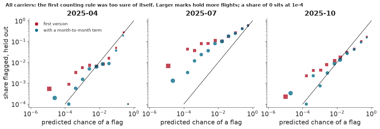
Perfect forecasts sit on the diagonal. Both versions sit above it at the low end, where the first version promised less than one flag in 10,000 flights and saw far more. The fix helps most in July, the worst month, lifting the mean log score from -0.329 to -0.270, and leaves April and October almost unchanged. It is not free: in the calm months the expected number of flags rises further above the truth, 156 against 85 in April and 325 against 195 in October, and July is still far short, 548 against 1,686. Neither version saw a month that bad coming.
Neither rule wins the national top 50. R0 caught 4, 36 and 20 flagged flights in the three months, R1 9, 35 and 9. With 0.4-8% of flights flagged, a random list of 50 would catch 0.2 to 3.9. That is the analyst's case, for under a second of machine time.
Those counts lean on the target month's own schedule. A real list has only last month's file, so it must rank last month's eligible flights at last month's operations. Built that way, R0 caught 4, 35 and 15 and R1 6, 31 and 6; up to 27 of R1's look-ahead 50 were flights a real list could not have named. Over all 12 months with a full window, the two are level when they can see the target month's schedule, 158 hits against 147, with R0 ahead in 5 months and R1 in 6. From last month's file alone R0 leads, 130 against 103, ahead in 7 months against 4. Yet R1 has the better log score in 11 of 12. R0 ranks a list better, and R1 states a chance better.
6 · R2 on one carrier
R2 models each flight x month cell. On the logit scale, a flight's late rate is a carrier level plus effects for origin, destination, flight and month, and a beta-binomial concentration $\phi$ carries the variation that is left:
$$\text{late}_{ft} \sim \text{BetaBinomial}\big(n_{ft},\ p_{ft}\phi,\ (1-p_{ft})\phi\big), \quad \text{logit}\, p_{ft} = a + \sigma_o z_{o[f]} + \sigma_d z_{d[f]} + \sigma_f z_f + m_t .$$
The flight, origin and destination effects are written non-centred, the scales get LogNormal priors
(E86 saw half-normal priors on scales run away under MEADS), and the month effect is a
pm.ZeroSumNormal. We sample with nutpie, 4 chains of 1,000 tuning steps and 1,000 draws, rather
than nutpie's default of 400 tuning steps. The centred form was not compared.
A national R2 does not fit in a reader's run: on 2 CPU cores it prices in hours (part 8), and on the card here a national run would break a 60-second limit on GPU jobs, with no way to checkpoint warmup. So we fit one carrier, the 8th of 15 by eligible cells, chosen by size alone, with every eligible flight it ran in the window. A prior predictive check in NumPy comes first.
sizes = np.bincount(cells.loc[window(TARGETS[0]), "carrier"], minlength=15)
CARRIER = int(np.argsort(-sizes)[7])  # 8th of 15 by eligible cells before the first target: chosen by size alone
print(f"The carrier holds {sizes[CARRIER] / sizes.sum():.1%} of the eligible cells in the first window.")
typical = []
for t in TARGETS:
    seen = cells[window(t)]
    for name, part, group in (("this carrier", targets_of(t, CARRIER), seen[seen["carrier"] == CARRIER]), ("all carriers", targets_of(t), seen)):
        typical.append({"target": TARGET_NAMES[t], "group": name, "window cells per flight": len(group) / group["flight"].nunique(),
                        "target flights with no history": 1 - part["flight"].isin(group["flight"]).mean(),
                        "flags on flights not eligible last month": f"{int((part['flagged'] & (part['state'] == -1)).sum())} of {int(part['flagged'].sum())}"})
print(pd.DataFrame(typical).set_index(["target", "group"]).round(2).to_string())


def r2_cells(target, carrier=CARRIER):
    w = cells[window(target) & (cells["carrier"] == carrier)]
    return w["flight"].to_numpy(), w["month"].to_numpy() - (target - WINDOW), w["n"].to_numpy(), w["late"].to_numpy()


def r2_model(f, m, n, k):
    """R2: late or cancelled in a flight x month cell, beta-binomial, flight effects written non-centred."""
    flights, fi = np.unique(f, return_inverse=True)
    origins, oi = np.unique(flight_origin[flights], return_inverse=True)
    dests, di = np.unique(flight_dest[flights], return_inverse=True)
    coords = {"flight": np.arange(flights.size), "origin": np.arange(origins.size), "dest": np.arange(dests.size),
              "month": np.arange(WINDOW)}
    with pm.Model(coords=coords) as model:
        a = pm.Normal("a", -1.7, 1.0)
        s_o = pm.LogNormal("s_o", np.log(0.2), 0.6)
        s_d = pm.LogNormal("s_d", np.log(0.2), 0.6)
        s_f = pm.LogNormal("s_f", np.log(0.3), 0.6)
        s_m = pm.LogNormal("s_m", np.log(0.3), 0.6)
        z_o = pm.Normal("z_o", 0.0, 1.0, dims="origin")
        z_d = pm.Normal("z_d", 0.0, 1.0, dims="dest")
        z_f = pm.Normal("z_f", 0.0, 1.0, dims="flight")
        month_effect = pm.ZeroSumNormal("m", sigma=s_m, dims="month")
        phi = pm.LogNormal("phi", np.log(30.0), 1.0)
        base = a + s_o * z_o[oi] + s_d * z_d[di] + s_f * z_f
        p = pm.math.invlogit(base[fi] + month_effect[m])
        pm.BetaBinomial("y", n=n, alpha=p * phi, beta=(1 - p) * phi, observed=k)
    return model, flights, origins, dests, oi, di


# Prior predictive, in NumPy on the first window: do these priors allow what this carrier really did?
f_, m_, n_, k_ = r2_cells(TARGETS[0])
flights_, fi_ = np.unique(f_, return_inverse=True)
oi_ = np.unique(flight_origin[flights_], return_inverse=True)[1]
di_ = np.unique(flight_dest[flights_], return_inverse=True)[1]
draws = 400
prior_rng = np.random.default_rng(RANDOM_SEED)
scale = lambda mean: prior_rng.lognormal(np.log(mean), 0.6, size=(draws, 1))
eta = (prior_rng.normal(-1.7, 1.0, size=(draws, 1))
       + (scale(0.2) * prior_rng.normal(size=(draws, oi_.max() + 1)))[:, oi_]
       + (scale(0.2) * prior_rng.normal(size=(draws, di_.max() + 1)))[:, di_]
       + scale(0.3) * prior_rng.normal(size=(draws, flights_.size)))
eta = eta[:, fi_] + (scale(0.3) * prior_rng.normal(size=(draws, WINDOW)))[:, m_]
phi_prior = prior_rng.lognormal(np.log(30.0), 1.0, size=(draws, 1))
mean_prior = expit(eta)
y_prior = prior_rng.binomial(n_, prior_rng.beta(mean_prior * phi_prior, (1 - mean_prior) * phi_prior))
share_prior, flagged_prior = (y_prior.sum(1) / n_.sum()), ((y_prior / n_) > 0.5).mean(1)
print(f"Prior predictive: late share {np.quantile(share_prior, 0.05):.2f}-{np.quantile(share_prior, 0.95):.2f} "
      f"(observed {k_.sum() / n_.sum():.2f}); flagged cells {np.quantile(flagged_prior, 0.05):.1%}-{np.quantile(flagged_prior, 0.95):.1%} "
      f"(observed {(k_ / n_ > 0.5).mean():.1%})")
del eta, mean_prior, y_prior


def fit_r2(target, carrier=CARRIER, tune=TUNE, draws=DRAWS, seed=None):
    """One fit, with real gradient counts, and checks on a stand-in for the list as well as on parameters."""
    f, m, n, k = r2_cells(target, carrier)
    model, flights, origins, dests, oi, di = r2_model(f, m, n, k)
    began = time.perf_counter()
    compiled = nutpie.compile_pymc_model(model)
    trace = nutpie.sample(compiled, chains=4, cores=CHAINS_AT_ONCE, tune=tune, draws=draws, progress_bar=False, save_warmup=True,
                          store_mass_matrix=False, seed=RANDOM_SEED + target if seed is None else seed)
    seconds = time.perf_counter() - began
    post = trace.posterior
    keep = {v: post[v].values.reshape(-1, *post[v].shape[2:]) for v in ("a", "s_o", "s_d", "s_f", "s_m", "phi", "z_o", "z_d", "z_f")}
    base = keep["a"][:, None] + keep["s_o"][:, None] * keep["z_o"][:, oi] + keep["s_d"][:, None] * keep["z_d"][:, di] + keep["s_f"][:, None] * keep["z_f"]
    ranked = np.argsort(-base.mean(0))[:50]
    logit_mean = xr.Dataset({"x": (("chain", "draw", "flight"), base[:, ranked].reshape(4, draws, 50))})
    hyper = xr.Dataset({v: (("chain", "draw"), post[v].values) for v in ("a", "s_o", "s_d", "s_f", "s_m", "phi")})
    out = {"target": target, "flights": flights, "origins": origins, "dests": dests, "fi": np.unique(f, return_inverse=True)[1],
           "month": m, "n": n, "late": k, "keep": keep, "seconds": seconds,
           "stats": {"cells": n.size, "flights": flights.size, "d": sum(v.size for v in model.initial_point().values()),
                     "seconds": seconds, "gradients warmup": int(trace.warmup_sample_stats["n_steps"].values.sum()),
                     "gradients draws": int(trace.sample_stats["n_steps"].values.sum()),
                     "divergences": int(trace.sample_stats["diverging"].values.sum()),
                     "max r_hat top 50": float(np.asarray(az.rhat(logit_mean)["x"]).max()),
                     "min ESS top 50": float(np.asarray(az.ess(logit_mean, method="bulk")["x"]).min()),
                     "max r_hat hyper": max(float(az.rhat(hyper)[v]) for v in hyper.data_vars),
                     "min ESS hyper": min(float(az.ess(hyper, method="bulk")[v]) for v in hyper.data_vars)}}
    del trace, compiled, post, model, base, logit_mean
    gc.collect()
    return out


def effect(rng_, scale_, z, codes, known_codes):
    """Posterior effect for codes seen in training; a new draw from the same sd for those that were not."""
    position = np.searchsorted(known_codes, codes).clip(0, known_codes.size - 1)
    known = known_codes[position] == codes
    out = scale_[:, None] * rng_.normal(size=(scale_.size, codes.size))
    out[:, known] = scale_[:, None] * z[:, position[known]]
    return out


def r2_forecast(fit, carrier=CARRIER, seed=None):
    """Flag probabilities for next month's flights: the plain version, and the one that redraws the month."""
    target, keep = fit["target"], fit["keep"]
    part = targets_of(target, carrier)
    flight, n = part["flight"].to_numpy(), part["n"].to_numpy()
    rng_ = np.random.default_rng([RANDOM_SEED, target] if seed is None else [RANDOM_SEED, target, 1000 + seed])
    base = (keep["a"][:, None] + effect(rng_, keep["s_o"], keep["z_o"], flight_origin[flight], fit["origins"])
            + effect(rng_, keep["s_d"], keep["z_d"], flight_dest[flight], fit["dests"])
            + effect(rng_, keep["s_f"], keep["z_f"], flight, fit["flights"]))
    plain = stats.binom.sf(n // 2, n, expit(base))
    month_shock = keep["s_m"][:, None] * rng_.normal(size=(keep["s_m"].size, 1))
    mean = expit(base + month_shock)
    rate = rng_.beta(mean * keep["phi"][:, None], (1 - mean) * keep["phi"][:, None])
    redrawn = stats.binom.sf(n // 2, n, rate)
    count = (rng_.binomial(n, rate) / n > 0.5).sum(1)
    half = redrawn.shape[0] // 2
    return {"table": part, "plain": plain.mean(0), "R2": redrawn.mean(0), "count": count, "plain_count": (rng_.binomial(n, expit(base)) / n > 0.5).sum(1),
            "half_a": redrawn[:half].mean(0), "half_b": redrawn[half:].mean(0), "sum_by_draw": redrawn.sum(1)}


def replicated_checks(fit, sims=400):
    """Training-window checks that redraw every month and all overdispersion. Flights keep their fitted effects."""
    keep, rng_ = fit["keep"], np.random.default_rng([RANDOM_SEED, fit["target"], 1])
    sims = min(sims, keep["a"].size)
    pick = rng_.choice(keep["a"].size, sims, replace=False)
    oi = np.unique(flight_origin[fit["flights"]], return_inverse=True)[1]
    di = np.unique(flight_dest[fit["flights"]], return_inverse=True)[1]
    base = (keep["a"][pick, None] + keep["s_o"][pick, None] * keep["z_o"][pick][:, oi] + keep["s_d"][pick, None] * keep["z_d"][pick][:, di]
            + keep["s_f"][pick, None] * keep["z_f"][pick])
    mean = expit(base[:, fit["fi"]] + (keep["s_m"][pick, None] * rng_.normal(size=(sims, WINDOW)))[:, fit["month"]])
    phi = keep["phi"][pick, None]
    y = rng_.binomial(fit["n"], rng_.beta(mean * phi, (1 - mean) * phi))
    monthly = lambda late, flag: (np.array([late[..., fit["month"] == t].sum(-1) / fit["n"][fit["month"] == t].sum() for t in range(WINDOW)]),
                                  np.array([flag[..., fit["month"] == t].mean(-1) for t in range(WINDOW)]))
    rep_late, rep_flag = monthly(y, y / fit["n"] > 0.5)
    obs_late, obs_flag = monthly(fit["late"], fit["late"] / fit["n"] > 0.5)
    checks = {"month-to-month sd of late share": (rep_late.std(0), obs_late.std()), "worst month's flagged share": (rep_flag.max(0), obs_flag.max()),
              "mean flagged share": (rep_flag.mean(0), obs_flag.mean())}
    return {name: {"observed": o, "replicated 5%": np.quantile(r, 0.05), "replicated 95%": np.quantile(r, 0.95), "P(rep >= obs)": (r >= o).mean()}
            for name, (r, o) in checks.items()}, obs_flag


with stage("R2, one carrier, 3 fits"):
    forecasts, other_seeds, diagnostics, ppc, training_months = {}, {}, {}, {}, {}
    for t in TARGETS:
        fit = fit_r2(t)
        forecasts[t] = r2_forecast(fit)
        other_seeds[t] = [r2_forecast(fit, seed=s)["R2"] for s in range(12)]  # the same draws, other forecast noise
        diagnostics[TARGET_NAMES[t]] = fit["stats"]
        ppc[TARGET_NAMES[t]], training_months[t] = replicated_checks(fit)
        del fit
        gc.collect()
print(pd.DataFrame(diagnostics).round(3).to_string())
print(pd.concat({k: pd.DataFrame(v).T for k, v in ppc.items()}).round(3).to_string())
The carrier holds 3.9% of the eligible cells in the first window.
                      window cells per flight  target flights with no history flags on flights not eligible last month
target  group
2025-04 this carrier                     1.91                            0.50                                  8 of 11
        all carriers                     3.41                            0.22                                 40 of 85
2025-07 this carrier                     1.73                            0.66                                 31 of 39
        all carriers                     3.20                            0.11                              297 of 1686
2025-10 this carrier                     1.65                            0.41                                   1 of 3
        all carriers                     3.31                            0.25                                94 of 195
Prior predictive: late share 0.04-0.47 (observed 0.16); flagged cells 0.0%-42.9% (observed 3.2%)
                     2025-04     2025-07     2025-10
cells               9627.000    9313.000    8485.000
flights             5042.000    5398.000    5131.000
d                   5180.000    5535.000    5274.000
seconds              239.760     236.805     211.478
gradients warmup  121034.000  124592.000  119902.000
gradients draws   123248.000  124000.000  124000.000
divergences            0.000       0.000       0.000
max r_hat top 50       1.005       1.006       1.006
min ESS top 50      6120.818    6461.162    6251.626
max r_hat hyper        1.007       1.005       1.010
min ESS hyper        723.364     616.727     610.497
                                         observed  replicated 5%  replicated 95%  P(rep >= obs)
2025-04 month-to-month sd of late share     0.057          0.028           0.080          0.305
        worst month's flagged share         0.151          0.031           0.226          0.120
        mean flagged share                  0.030          0.012           0.046          0.230
2025-07 month-to-month sd of late share     0.055          0.026           0.081          0.268
        worst month's flagged share         0.151          0.032           0.210          0.115
        mean flagged share                  0.031          0.012           0.043          0.180
2025-10 month-to-month sd of late share     0.028          0.017           0.047          0.510
        worst month's flagged share         0.066          0.019           0.078          0.098
        mean flagged share                  0.018          0.009           0.022          0.128
This carrier is not typical, and its size did not show it. It holds 3.9% of the eligible cells, but its flights are short-lived: 1.7-1.9 window cells a flight against 3.2-3.4 nationally. 41-66% of its target flights have no history in the window, and so no fitted effect of their own, against 11-25% nationally, and 31 of July's 39 flags fell on flights that were not eligible the month before. What follows is therefore less a test of flight history than of how R2 treats new flights.
The priors allow a late share of 4-47% and flagged cells up to 43%, wide around the observed 16% and 3%. The fits are clean: no divergences, $\hat R$ at most 1.01 (1.0104 on one October hyperparameter), and bulk ESS above 6,000 on the logit means of the 50 flights ranked highest in training and above 600 on the hyperparameters. Each fit takes about 4 minutes and spends about 60,000 gradients a chain, warmup and sampling together.
The checks on the training window redraw all 12 month effects and all the overdispersion, keeping the flights' fitted effects. Observed values sit inside the 5-95% range on all three measures in all three windows, with $P(\text{rep} \ge \text{obs})$ from 0.10 to 0.51. Keeping the flight effects makes this a weak test: it says the spread between months is plausible, not that the forecasts are good. Only held-out months can say that.
Failure 3: forecasting an average month
The obvious forecast takes each flight's fitted effects, sets the month effect to its mean of zero, and reads off the chance of passing 50%. But next month is a new month. The right forecast draws a new month effect from the fitted spread $\sigma_m$, new overdispersion from $\phi$, and, for flights and airports the window never saw, new effects from the fitted scales.
for t, f in forecasts.items():
    part = f["table"]
    f["R0"] = r0_forecast(t, CARRIER)
    f["R1"] = r1_forecast(t, CARRIER)
    f["tie"] = tie_break(part, t)
rows = []
for t, f in forecasts.items():
    flagged = f["table"]["flagged"].to_numpy()
    rows.append({"target": TARGET_NAMES[t], "flights": flagged.size, "flagged": int(flagged.sum()),
                 "first version, expected": f["plain"].sum(), "first version, score": log_score(f["plain"], flagged).mean(),
                 "redrawn, expected": f["R2"].sum(), "redrawn, 5%": np.quantile(f["count"], 0.05), "redrawn, 95%": np.quantile(f["count"], 0.95),
                 "redrawn, score": log_score(f["R2"], flagged).mean(),
                 "list overlap, two halves of the draws": len(set(top(f["half_a"], LIST_SIZE)) & set(top(f["half_b"], LIST_SIZE)))})
print(pd.DataFrame(rows).set_index("target").T.round(3).to_string())

fig, ax = plt.subplots(figsize=(10.5, 4.6), layout="constrained")
for row, (t, f) in enumerate(forecasts.items()):
    y = 2 - row
    total = len(f["table"])
    for shift, counts, colour in ((0.15, f["count"], MEASURED), (-0.15, f["plain_count"], ALARM)):
        low, mid, high = np.quantile(counts, [0.05, 0.5, 0.95])
        ax.plot([low + 0.5, high + 0.5], [y + shift] * 2, color=colour, lw=6, alpha=0.75, solid_capstyle="butt")
        ax.scatter([mid + 0.5], [y + shift], s=45, color="w", edgecolor=colour, lw=1.6, zorder=3)
    ax.scatter([f["table"]["flagged"].sum() + 0.5], [y], marker="D", s=70, color="k", zorder=4)
    ax.plot(training_months[t] * total + 0.5, np.full(WINDOW, y + 0.37), "|", color="#33424b", ms=9, mew=1.4)
ax.set(xscale="log", xlim=(0.4, 200), ylim=(-0.6, 2.6), yticks=[2, 1, 0], xlabel="flights flagged next month on this carrier (plotted at count + 0.5)")
ax.set_yticklabels(TARGET_NAMES.values())
ax.set_xticks([0.5, 1.5, 5.5, 10.5, 30.5, 100.5], ["0", "1", "5", "10", "30", "100"])
ax.xaxis.set_minor_formatter(NullFormatter())
ax.legend(handles=[Line2D([], [], color=MEASURED, lw=6, alpha=0.75, label="90% interval, month and overdispersion redrawn"),
                   Line2D([], [], color=ALARM, lw=6, alpha=0.75, label="90% interval, an average month"),
                   Line2D([], [], marker="o", ls="", markerfacecolor="w", markeredgecolor="#33424b", markeredgewidth=1.6, ms=7,
                          label="median of either interval"),
                   Line2D([], [], marker="D", ls="", color="k", label="what happened"),
                   Line2D([], [], marker="|", ls="", color="#33424b", ms=9, mew=1.4, label="the 12 training months, scaled to this list")],
          loc="lower right", fontsize=8.5)
ax.set_title("A forecast that keeps an average month cannot see a bad one", loc="left", fontsize=11);
target                                 2025-04  2025-07  2025-10
flights                                675.000  593.000  500.000
flagged                                 11.000   39.000    3.000
first version, expected                  6.753    6.577    3.364
first version, score                    -0.078   -0.257   -0.030
redrawn, expected                       16.061   13.723    6.223
redrawn, 5%                              0.000    0.000    0.000
redrawn, 95%                            58.000   46.000   18.000
redrawn, score                          -0.077   -0.217   -0.033
list overlap, two halves of the draws    9.000   10.000   10.000
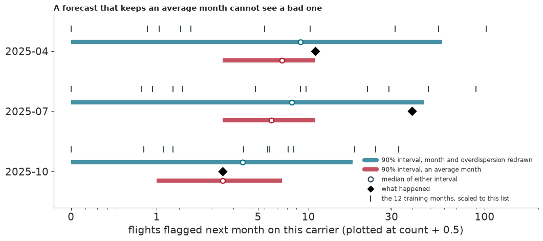
The first version is sure of a narrow count and misses July: it expects about 7 flags where 39 happened. The redrawn forecast admits what it does not know, with 90% intervals from 0 to 18-58 flags, and July's 39 falls inside. Its mean is still only about 14, because a new month is drawn from all months alike: the model does not know July is a bad month, though its window held July 2024 with 1,562 flags and June 2025 with 1,312. A seasonal month effect is the obvious next step, and R2 does not have one. Honesty also has a price in the score: the redrawn forecast is better by 0.040 in July, level in April and 0.003 worse in October.
Two halves of the posterior draws give lists of 10 that share 9-10 flights, so the list is steady under Monte Carlo noise. That does not settle a rule that can turn on one flight, which part 7 tests.
7 · Does the bigger model change the list?
For the carrier's list we use 10 flights, not the charity's 50: 50 of about 600 flights is far less selective than 50 of 20,000 nationally. To choose between R0, R1 and R2 in each test month we take the cheapest model whose mean log score is within one bootstrap standard error of the best (resampling origin airports). It must also share at least 8 of its 10 flights with the next model up. Where the months disagree, two of three decide. The list of 50 is printed too, but it decides nothing.
The rule was fixed before any score was read, but not blind. The flag counts of the test months had already been seen as data checks, and along the way the list it judges was shortened from 50 to 10. The length matters: 10 is the only length we tried where R1 wins any month. A list of 20 gives R2 in all three months, and at 50 R1's overlap of 20-28 misses the 80% bar.
def decide(list_size=LIST_SIZE, needed=NEEDED, resamples=2000):
    """The rung rule, written down before any score was read, applied to each origin in turn."""
    rows, picks = [], {}
    for t, f in forecasts.items():
        part = f["table"]
        flagged = part["flagged"].to_numpy()
        airports = flight_origin[part["flight"].to_numpy()]
        codes, inverse = np.unique(airports, return_inverse=True)
        scores = {r: log_score(f[r], flagged) for r in ("R0", "R1", "R2")}
        means = {r: s.mean() for r, s in scores.items()}
        best = max(means, key=means.get)
        count = np.bincount(inverse)
        boot = np.random.default_rng([RANDOM_SEED, t]).integers(codes.size, size=(resamples, codes.size))
        se = {}
        for r, s in scores.items():
            gap = np.bincount(inverse, s - scores[best])
            se[r] = (gap[boot].sum(1) / count[boot].sum(1)).std()
        lists = {"R0": top(f["R0"], list_size, f["tie"]), "R1": top(f["R1"], list_size), "R2": top(f["R2"], list_size)}
        shared = {"R0": len(set(lists["R0"]) & set(lists["R1"])), "R1": len(set(lists["R1"]) & set(lists["R2"])), "R2": list_size}
        passes = {r: (means[best] - means[r] <= se[r]) and shared[r] >= needed for r in ("R0", "R1", "R2")}
        pick = next((r for r in ("R0", "R1", "R2") if passes[r]), None)
        picks[t] = pick or best
        for r in ("R0", "R1", "R2"):
            rows.append({"target": TARGET_NAMES[t], "rung": r, "log score": means[r], "gap to best": means[best] - means[r], "one SE": se[r],
                         f"hits in top {list_size}": int(flagged[lists[r]].sum()), "shared with next rung": shared[r], "passes": passes[r]})
        rows[-1]["picked"] = picks[t] if pick else f"{best} (none passed)"
    return pd.DataFrame(rows).set_index(["target", "rung"]), picks


with stage("scores"):
    verdict, picks = decide()
print(verdict.round(4).to_string())
print("Picks by origin:", {TARGET_NAMES[t]: r for t, r in picks.items()})
print("With a list of 50, which decides nothing:")
print(decide(list_size=50, needed=40)[0][["hits in top 50", "shared with next rung"]].unstack("rung").to_string())


def hit_gap(t, k=50, resamples=2000):
    """R2's extra hits over R1 in a list of k, with a 5-95% range from resampling origin airports."""
    f = forecasts[t]
    part, flagged = f["table"], f["table"]["flagged"].to_numpy(float)
    gain = np.zeros(flagged.size)
    gain[top(f["R2"], k)] += flagged[top(f["R2"], k)]
    gain[top(f["R1"], k)] -= flagged[top(f["R1"], k)]
    codes, inverse = np.unique(flight_origin[part["flight"].to_numpy()], return_inverse=True)
    boot = np.random.default_rng([RANDOM_SEED, t, 2]).integers(codes.size, size=(resamples, codes.size))
    low, high = np.quantile(np.bincount(inverse, gain)[boot].sum(1), [0.05, 0.95])
    return {"R2 less R1 hits": int(gain.sum()), "5%": low, "95%": high}


print("Top 50, airports resampled:", {TARGET_NAMES[t]: hit_gap(t) for t in TARGETS})
overlaps = {TARGET_NAMES[t]: [len(set(top(forecasts[t]["R1"], LIST_SIZE)) & set(top(p, LIST_SIZE))) for p in other_seeds[t]] for t in TARGETS}
print("R1 and R2 lists of 10 shared, on 12 other forecast seeds:", overlaps)
print("R2 hits in the top 50 on those seeds:", {TARGET_NAMES[t]: sorted({int(forecasts[t]["table"]["flagged"].to_numpy()[top(p, 50)].sum()) for p in other_seeds[t]})
                                                for t in TARGETS})
history = pd.DataFrame([{"target": TARGET_NAMES[t], "R1 12 months, all carriers": national_table.loc[TARGET_NAMES[t], "R1 score"],
                         "R1 3 months, all carriers": log_score(r1_forecast(t, months=3), national[t]["table"]["flagged"].to_numpy()).mean(),
                         "R1 12 months, this carrier": log_score(forecasts[t]["R1"], forecasts[t]["table"]["flagged"].to_numpy()).mean(),
                         "R1 3 months, this carrier": log_score(r1_forecast(t, CARRIER, months=3), forecasts[t]["table"]["flagged"].to_numpy()).mean(),
                         "R2, this carrier": log_score(forecasts[t]["R2"], forecasts[t]["table"]["flagged"].to_numpy()).mean()} for t in TARGETS]).set_index("target")
print(history.T.round(4).to_string())

fig, axes = plt.subplots(1, 3, figsize=(12.4, 6.3), sharey=True, layout="constrained")
LIMIT_RANK = 30
for ax, (t, f) in zip(axes, forecasts.items()):
    flagged = f["table"]["flagged"].to_numpy()
    ranks = {r: np.argsort(np.lexsort((-f["tie"] if r == "R0" else np.zeros(flagged.size), -f[r]))) + 1 for r in ("R0", "R1", "R2")}
    chosen = sorted(set().union(*(np.flatnonzero(v <= LIST_SIZE) for v in ranks.values())), key=lambda i: flagged[i])
    for i in chosen:
        y = [min(ranks[r][i], LIMIT_RANK) for r in ("R0", "R1", "R2")]
        hit = flagged[i]
        ax.plot(range(3), y, "-o", ms=5 if hit else 3.5, lw=2.2 if hit else 1, color=ALARM if hit else "#a9b7bf", alpha=0.95 if hit else 0.8, zorder=3 if hit else 2)
    ax.axhline(LIST_SIZE + 0.5, color="k", lw=0.8, ls=":")
    ax.set(xticks=range(3), xticklabels=["R0", "R1", "R2"], title=f"{TARGET_NAMES[t]}: {int(flagged.sum())} of {flagged.size} flagged", xlim=(-0.25, 2.25))
axes[0].set(ylim=(LIMIT_RANK + 1, 0), ylabel=f"rank on the carrier's list ({LIMIT_RANK} means {LIMIT_RANK} or lower)")
axes[-1].annotate("list\nends\nhere", (1, LIST_SIZE + 0.5), xycoords=("axes fraction", "data"), xytext=(5, 0),
                  textcoords="offset points", va="center", fontsize=9, annotation_clip=False)
fig.legend(handles=[Line2D([], [], color=ALARM, lw=2.2, marker="o", label="flagged, held out"),
                    Line2D([], [], color="#a9b7bf", lw=1, marker="o", label="not flagged")], loc="outside lower center", ncols=2, fontsize=9)
fig.suptitle("Every flight on any rung's list. Red lines are the flights that really were flagged", x=0.01, ha="left", fontsize=11);
              log score  gap to best  one SE  hits in top 10  shared with next rung  passes picked
target  rung
2025-04 R0      -0.0829       0.0057  0.0066               0                      1   False    NaN
        R1      -0.0840       0.0068  0.0094               0                      8    True    NaN
        R2      -0.0772       0.0000  0.0000               0                     10    True     R1
2025-07 R0      -0.2655       0.0488  0.0115               2                      4   False    NaN
        R1      -0.2481       0.0314  0.0091               4                      8   False    NaN
        R2      -0.2167       0.0000  0.0000               4                     10    True     R2
2025-10 R0      -0.0427       0.0098  0.0038               0                      0   False    NaN
        R1      -0.0358       0.0029  0.0049               0                      7   False    NaN
        R2      -0.0329       0.0000  0.0000               0                     10    True     R2
Picks by origin: {'2025-04': 'R1', '2025-07': 'R2', '2025-10': 'R2'}
With a list of 50, which decides nothing:
        hits in top 50         shared with next rung
rung                R0  R1  R2                    R0  R1  R2
target
2025-04              0   0   3                     4  20  50
2025-07              4  10  17                     9  25  50
2025-10              0   0   2                     7  28  50
Top 50, airports resampled: {'2025-04': {'R2 less R1 hits': 3, '5%': np.float64(0.0), '95%': np.float64(7.0)}, '2025-07': {'R2 less R1 hits': 7, '5%': np.float64(0.0), '95%': np.float64(14.0)}, '2025-10': {'R2 less R1 hits': 2, '5%': np.float64(0.0), '95%': np.float64(5.0)}}
R1 and R2 lists of 10 shared, on 12 other forecast seeds: {'2025-04': [8, 8, 8, 8, 7, 8, 8, 8, 8, 8, 8, 8], '2025-07': [8, 8, 8, 8, 8, 8, 8, 8, 8, 8, 8, 8], '2025-10': [7, 7, 7, 7, 7, 7, 7, 7, 7, 7, 7, 7]}
R2 hits in the top 50 on those seeds: {'2025-04': [3], '2025-07': [17], '2025-10': [2]}
target 2025-04 2025-07 2025-10 R1 12 months, all carriers -0.0258 -0.2704 -0.0479 R1 3 months, all carriers -0.0278 -0.2404 -0.0552 R1 12 months, this carrier -0.0840 -0.2481 -0.0358 R1 3 months, this carrier -0.0940 -0.2390 -0.0397 R2, this carrier -0.0772 -0.2167 -0.0329
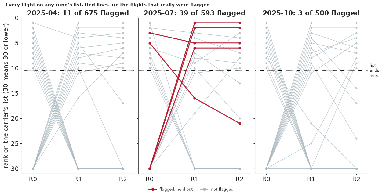
The rule picks R1 in April and R2 in July and October, so R2 for this carrier, but the margins are thin. Only in July is R2's gain larger than its noise: a gap of 0.031 in mean log score against a standard error of 0.009. In April and October R1 is within one standard error, and in October it fails only on overlap, by one flight: 7 shared where 8 are needed. Had one flight moved in October, the answer on this carrier would be R1.
April's pick is fragile too: R1 sits right on the overlap bar, and a few other seeds move it to R2, so R2 for this carrier holds either way.
Only July is evidence that R2 is better, and part of that may be R1's slow 12-month window: a 3-month R1 scores -0.239 against R2's -0.217 on this carrier, where the 12-month R1 scores -0.248. The overlap test measures difference, not benefit, so in October R2 is bought with a score gap inside one standard error and 0 hits against 0. A short window is no free gain either: it is worse in the calm months (-0.055 against -0.048 nationally in October).
So yes, the list changes: R1 and R2 share 7-8 of 10 flights and 20-28 of 50. Whether that helps depends on the length. In a list of 10 both catch the same 0, 4 and 0 flagged flights, and the 11 flags of April and 3 of October fall outside every list of 10. In a list of 50 R2 catches 3, 17 and 2 against R1's 0, 10 and 0. July's gain of 7 is noisy: resampling airports gives a 5-95% range of about 0 to 14. On this carrier 50 is about a tenth of all flights, so the gain does not carry over to a national list of 50.
On the chart R0 barely overlaps anything, because it lists last month's flags. About half the lines run from R0's floor up into R1's list: going from one month of history to twelve is the largest change of rank on the page, for a tenth of a second. It is not the largest change in what the list catches, which comes from R1 to R2.
fig, axes = plt.subplots(1, 3, figsize=(12, 4.3), sharex=True, layout="constrained")
fit_seconds = {t: diagnostics[TARGET_NAMES[t]]["seconds"] for t in TARGETS}
for ax, (t, f) in zip(axes, forecasts.items()):
    seconds = [national[t]["seconds"]["R0"], national[t]["seconds"]["R1"], fit_seconds[t]]
    means = verdict.loc[TARGET_NAMES[t], "log score"].to_numpy()
    ax.step(seconds + [1e4], np.r_[np.maximum.accumulate(means), np.maximum.accumulate(means)[-1]], where="post", color="#b9c6cd", lw=2, zorder=1)
    for x, y, r in zip(seconds, means, ("R0", "R1", "R2")):
        ax.scatter([x], [y], s=95, color=RUNG_COLOUR[r], zorder=3)
        ax.annotate(r, (x, y), xytext=(0, 9), textcoords="offset points", ha="center", fontsize=10)
    ax.set(xscale="log", title=TARGET_NAMES[t])
    ax.margins(y=0.2)
axes[0].set_ylabel("held-out log score")
fig.supxlabel("machine seconds for this rung, 2 cores", fontsize=11)
fig.suptitle("Value for money, one carrier. R0 and R1 timed on all carriers, R2 on this one: a staircase climbs only when a rung pays", x=0.01, ha="left", fontsize=11);
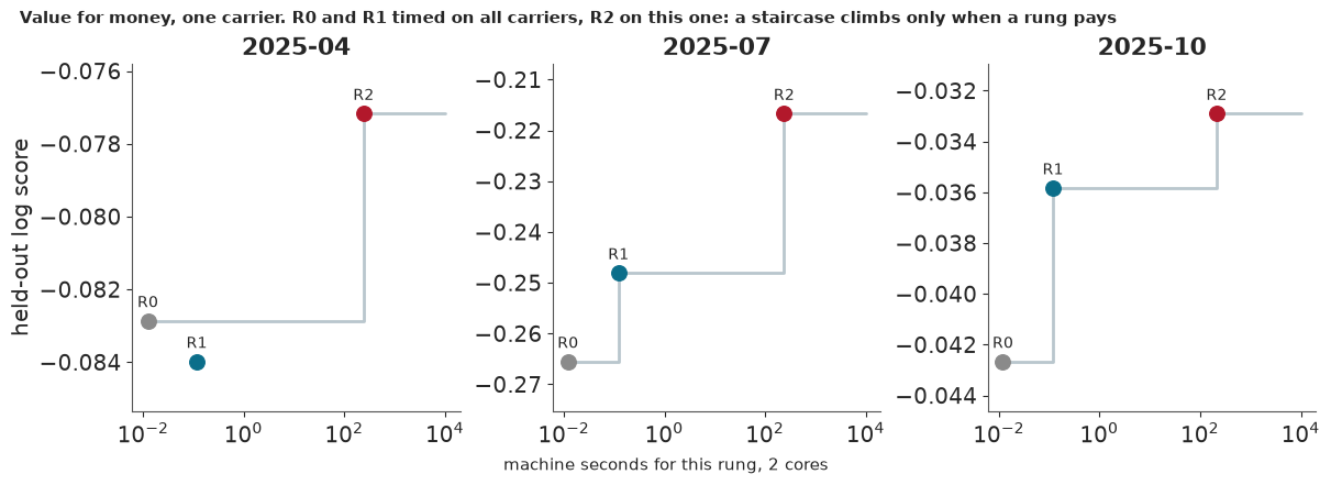
Each step up the staircase is a purchase, and a higher score is better. R1 costs about a tenth of a second on every carrier, and R2 about 4 minutes on this one. Each panel has its own vertical scale, because the months cannot be compared. In April R1 sits below R0 and buys nothing on score. Note the horizontal axis: R0 and R1 are timed on all carriers and R2 on one carrier, which flatters R2 by about 26x. Its national price is in the next table.
8 · What this run cost, and what to tell the charity
The last cell adds up what this run spent and prices every model, for one forecast and for the three test months. Each extrapolated line says what it rests on.
price = pd.Series(PRICE, name="seconds").round(0).astype(int)
print(price.to_string())
print(f"Total in stages: {price.sum() / 60:.1f} min on {CORES} cores")
assert {d.platform for d in jax.devices()} == {"cpu"}, "a reader's run must not start a GPU"
print("JAX saw CPU devices only, so this run used no GPU.")

r2_mean_s = np.mean([d["seconds"] for d in diagnostics.values()])
r2_cells_share = sizes.sum() / sizes[CARRIER]
gpu_three = f"{hours(r2_gpu_ms, 60_000, 3) * 60:.0f}-{hours(r2_gpu_ms, 160_000, 3) * 60:.0f} min"
window_three = [sum(hours(ms_14m * r / ROWS, g) for r in fit_rows["12-month window"]) for g in GRADIENTS]
ladder_of_prices = pd.DataFrame(
    [("R0, all carriers", f"{np.mean([f['seconds']['R0'] for f in national.values()]):.2f} s",
      f"{np.mean([f['seconds']['R0'] for f in national.values()]) * 3:.2f} s", "measured", "CPU, 2 cores"),
     ("R1, all carriers", f"{np.mean([f['seconds']['R1'] for f in national.values()]):.2f} s",
      f"{np.mean([f['seconds']['R1'] for f in national.values()]) * 3:.2f} s", "measured", "CPU, 2 cores"),
     ("R2, one carrier, nutpie", f"{r2_mean_s / 60:.1f} min", f"{r2_mean_s * 3 / 60:.0f} min", "measured", "CPU, 2 cores"),
     ("R2, all carriers, nutpie, every flight", f"{r2_mean_s * r2_cells_share / 3600:.1f} h or more", f"{r2_mean_s * r2_cells_share * 3 / 3600:.1f} h or more",
      "extrapolated", f"{r2_cells_share:.0f}x the cells, same gradient count; d about 14x larger"),
     ("R2, all carriers, 3-cell cut, ChEES", f"{hours(r2_gpu_ms, 60_000) * 60:.0f}-{hours(r2_gpu_ms, 160_000) * 60:.0f} min, plus extra restarts",
      f"{gpu_three}, plus extra restarts", "extrapolated", "measured gradient x assumed count; ChEES never run on R2"),
     ("R3, all rows, ChEES", f"{hours(ms_14m, 60_000):.1f}-{hours(ms_14m, 160_000):.1f} h, plus extra restarts",
      f"{window_three[0]:.1f}-{window_three[1]:.1f} h on the 12-month window", "extrapolated",
      "no float32 test, gradient count unmeasured, E86's recipe needs a 2,080 GiB table")],
    columns=["rung", "one forecast", "three test months", "label", "basis"]).set_index("rung")
print(ladder_of_prices.to_string())
print(f"One more tree doubling would make nutpie's three months about {r2_mean_s * r2_cells_share * 6 / 3600:.0f} h.")
timing_free = {k: {name: value for name, value in v.items() if name != "seconds"} for k, v in diagnostics.items()}
store.save_json("decide", {"verdict": verdict.reset_index().to_dict("list"), "picks": {TARGET_NAMES[t]: r for t, r in picks.items()},
                           "diagnostics": timing_free, "national": national_table.reset_index().to_dict("list")});
timing rows 1-5              9
row 5 ladder                 9
R0 and R1, all carriers      1
R2, one carrier, 3 fits    725
scores                       0
Total in stages: 12.4 min on 2 cores
JAX saw CPU devices only, so this run used no GPU.
                                                          one forecast                  three test months         label                                                                             basis
rung
R0, all carriers                                                0.01 s                             0.04 s      measured                                                                      CPU, 2 cores
R1, all carriers                                                0.12 s                             0.36 s      measured                                                                      CPU, 2 cores
R2, one carrier, nutpie                                        3.8 min                             11 min      measured                                                                      CPU, 2 cores
R2, all carriers, nutpie, every flight                   1.6 h or more                      4.9 h or more  extrapolated                            26x the cells, same gradient count; d about 14x larger
R2, all carriers, 3-cell cut, ChEES      5-14 min, plus extra restarts     16-43 min, plus extra restarts  extrapolated                          measured gradient x assumed count; ChEES never run on R2
R3, all rows, ChEES                     2.6-7.0 h, plus extra restarts  3.9-10.5 h on the 12-month window  extrapolated  no float32 test, gradient count unmeasured, E86's recipe needs a 2,080 GiB table
One more tree doubling would make nutpie's three months about 10 h.
The run took about 12 minutes, 725 seconds of it in the three fits of R2. R3's one forecast uses all 24 months, and its three test months the 12-month window. Both national versions of R2 are extrapolations, and neither is the R2 fitted here. ChEES on the cut model is a measured gradient times an assumed count, on a sampler never run on R2. Nutpie with every flight scales this carrier's time by 26x the cells at the same gradient count, with about 14x as many parameters. Timings vary between runs, hence the ranges, and a result as thin as part 7's can move on another machine.
How to write a price someone can check
A quote is a sentence with five parts: what is bought, on what hardware, measured from what, the range, and what would make it wrong. Compare
"Two hours on one GPU."
with
"One fit of the row-level model for one forecast month costs 2.6-7.0 hours on an RTX 3090 Ti at 32 chains, scaled 1.41x from a measured 10-million-row gradient of 112 ms, for 60,000-160,000 gradients. It takes longer if warmup must restart more than E86's did, if R3 needs more gradients than E86, or if float32 fails at 14 million rows. It needs a sampler that fits in memory at 747,000 parameters, which E86's recipe does not. Nobody has shown what it does to the list."
The second can be checked, argued with and refused. It is also the pattern for the rest of the large-model series: each notebook opens with its price and the smallest model that could answer the question, and says whether the big model changed the decision.
What to tell the charity
So the research lead should not sign the quote as written. A price they could check would give a measured gradient count, warmup included, a float32 test at 14 million rows, a sampler that fits in memory at this size, and three test months. Meanwhile the counting rules make a list tonight: rank by R0, print R1's chance beside each flight, and call it "likely to be flagged". Months, not models, will decide how good that list looks, since flags ran from 25 to 1,686 a month and nothing here saw July coming.
The one purchase worth making next is R2 on all carriers for the same three months, about 16-43 minutes on the GPU for the cut model or about 5 hours on 2 cores with every flight. That fits a night, though the CPU version has little room to spare: one more tree doubling makes it about 10 hours. If its national list adds nothing to R1's, the row-level question goes away.
The plain order of work is the lesson: price before you buy, measure before you claim, and let the smallest model that answers the question go first. It may be the answer.
Summary
- A price has three factors and two walls. Time is time per gradient x gradients x fits, and memory and precision must hold. The contractor's 0.15 s a gradient is right by accident, a rate 5x too slow per lookup applied to 5x too few lookups, but two hours holds only below about 46,000 gradients. One fit of R3 prices at 2.6-7.0 hours for 60,000-160,000 gradients, and a test on three months at 3.9-10.5 hours on a 12-month window. These are extrapolated from a gradient measured at 10M rows, both gradient counts are assumed, and R3 was never fitted.
- A rate belongs to a cost shape. The same card is about 30-35x cheaper than 2 CPU threads on
matched rows and about 200x dearer on a
scan. The CPU side is 2 threads of one Ryzen 5950X and the GPU one RTX 3090 Ti, so this is neither a GPU against a well-run CPU nor a speed for your laptop. - Collapse first, then measure. Collapsing rows into flight x month cells is worth about 15x a gradient. Sorting rows by flight, the planned fix, made one lookup at 10M rows 1.6-1.9x slower on the card, and a power law from small subsets hit the month only by straddling a step in the CPU timings.
- The walls a rate cannot see. Gradient memory is modest (about 5.7 GiB at 32 chains and 14M rows, scaled), but E86's ChEES warmup keeps a d x d table of about 2,080 GiB at R3's 747,000 parameters. Near R3's log density, float32 numbers are 0.5 nats apart; whether that harms a fit was not tested.
- The counting rules make a usable list today. Built from last month's file, R0's national top 50 caught 4, 35 and 15 flagged flights in the three test months and R1's 6, 31 and 6, against 0.2-3.9 for a random list. Over 12 months R0 ranks better (130 hits against 103) and R1 states chances better (11 of 12 log scores).
- Forecast a new month, not an average one. R2 with the month redrawn gives 90% intervals of 0 to 18-58 flags that cover July's 39, where the average-month version expected 7. It still cannot tell that July is a bad month.
- R2 changes the list, and helps a little. On one mid-size carrier (3.9% of the cells; no national R2 has run) with unusually many new flights, R1 and R2 share 7-8 of 10 flights and catch the same 0, 4 and 0 flags; in a list of 50 R2 catches 3, 17 and 2 against 0, 10 and 0. The rule fixed before scoring buys R2, but only July shows a clear gain, October turns on one flight and April's pick moves with the seed.
Try it yourself
Each of these runs as printed at the end of the notebook on 2 cores. The first two take under a second, the third about 75 seconds.
- A cost law from less.
predict_month(fit_days=(3, 7))andpredict_month(fit_days=(7, 14), chains=1)fit the law of part 3 on other sizes. One sits across the step and overshoots the month several times over; the other sits above it and lands within about 10%. Which is which, and could you have known in advance? - A longer list.
decide(list_size=20, needed=16)[1]reruns the rule with a list of 20 and the same 80% overlap, and it gives R2 in all three months. Printdecide(list_size=20, needed=16)[0]to see what changed for April. Why should a rule be fixed before reading the scores, list length included? - Another carrier. Take the 10th of 15 with
other = int(np.argsort(-sizes)[9]), fit it with fewer draws usingsmall_fit = fit_r2(TARGETS[1], carrier=other, tune=400, draws=300), then comparelog_score(r2_forecast(small_fit, other)["R2"], targets_of(TARGETS[1], other)["flagged"]).mean()withlog_score(r1_forecast(TARGETS[1], other), targets_of(TARGETS[1], other)["flagged"]).mean(). Readsmall_fit["stats"]first: at these short settings the hyperparameters' $\hat R$ is about 1.06, which fails the usual bar. One more carrier is one more story, not a national answer.