Hardware. The stored outputs come from one desktop: an NVIDIA RTX 3090 Ti and a 16-core Ryzen 5950X running on 15 cores. Without a GPU the notebook fits a coarser 20 m lattice and skips the GPU comparisons, so your numbers will differ from the prose. GPU runs are not bit-reproducible even with a fixed seed, so the prose gives rounded values, or ranges over repeated runs.
The setting
Barro Colorado Island in Panama holds one of the best-studied pieces of tropical forest in the world. In its 50-hectare plot, 1000 by 500 metres, every free-standing tree has been mapped and measured (Hubbell & Foster 1983; Condit et al. 1996). One species, Beilschmiedia pendula, is a classic of spatial statistics (Møller & Waagepetersen 2007): its 3,604 trees bunch into clumps and seem to favour some kinds of ground over others.
Suppose a forest ecologist asks two questions about it. Does the species' link to terrain hold across the whole plot, or only in parts of it? And which five hectares should a recruitment survey use, if the aim is the best habitat rather than wherever a clump of trees happens to stand?
The first question needs effects that vary over space. Both need us to separate habitat from the fine clustering of a species whose seeds fall near their parents. The natural model is a log-Gaussian Cox process (Møller, Syversveen & Waagepetersen 1998): a Poisson count in every cell of a lattice, with a log intensity built from Gaussian random fields. With four latent fields on a 5 m lattice, that is 20,000 cells and 24,810 parameters.
The model is also a fair test of a GPU, which is the second subject of this notebook, because every gradient is a stack of dense matrix products. A GPU does thousands of identical operations at once. One NUTS chain cannot use that, since each step depends on the one before it. Many chains can: a gradient for 128 chains is one big batched matrix product. With many chains, effective sample size is plentiful, and the limit moves to how fast the chains reach the posterior and mix through it (Hoffman, Radul & Sountsov 2021). ChEES-HMC and MEADS are built for that regime. They tune their settings from the ensemble itself, so that all chains take the same number of steps in lock-step. We pit them against a well-configured NUTS run on the CPU.
The plan
| part | question | tool |
|---|---|---|
| 1 | What do the trees look like, and what model fits them? | variance-to-mean ratios, Hilbert-space GPs |
| 2 | How fast is a good CPU sampler? | nutpie in float64 |
| 3 | Where does the time go on a GPU? | batched gradients: chains, size, precision |
| 4 | Can ChEES-HMC sample the model? | blackjax.chees_adaptation, culling stragglers |
| 5 | Why not just run NUTS on the GPU? | vectorised blackjax.nuts |
| 6 | What does MEADS add? | blackjax.meads_adaptation, a warm start |
| 7 | How large is the speed-up, and how much is hardware? | worst-case ESS per second |
| 8 | Is single precision safe? | float32 against float64 log densities |
| 9 | What does the model say about the forest? | posterior fields, a predictive check, hectare ranks |
| 10 | Which steps does a GPU speed up? | timing each stage |
import os

os.environ.setdefault("OPENBLAS_NUM_THREADS", "1")  # before NumPy: one BLAS thread per nutpie chain

import contextlib
import importlib.util
import logging
import tempfile
import time
import warnings

import arviz as az
import jax
import jax.numpy as jnp
import matplotlib.pyplot as plt
import numpy as np
import nutpie
import pandas as pd
import pymc as pm
import pytensor
import pytensor.tensor as pt
import xarray as xr
from jax.flatten_util import ravel_pytree
from pymc.sampling.jax import get_jaxified_graph, get_jaxified_logp

from pymc_challenges import data

RANDOM_SEED = 86
rng = np.random.default_rng(RANDOM_SEED)
az.style.use("arviz-variat")
warnings.filterwarnings("ignore", message=".*Explicitly requested dtype.*")
warnings.filterwarnings("ignore", message=".*truncated to dtype float32.*")
logging.getLogger("pymc").setLevel(logging.WARNING)

# Asking JAX for its backend would start CUDA, and the CPU baseline comes first. So does importing blackjax, which
# touches a JAX array when it loads: its import waits until after the baseline, against the usual first-cell habit.
HAS_GPU = (importlib.util.find_spec("jax_cuda13_plugin") is not None
           and any(os.path.exists(d) for d in ("/dev/nvidia0", "/dev/nvidiactl", "/dev/dxg"))
           and os.environ.get("JAX_PLATFORMS") != "cpu")
CORES = len(os.sched_getaffinity(0)) if hasattr(os, "sched_getaffinity") else os.cpu_count()
NUTS_CHAINS = min(8, max(4, CORES // 2 - 1))  # one on each physical core, capped to keep the build under 5 GB
NUTS_DRAWS = 4000 // NUTS_CHAINS               # 4,000 draws in total
L_SMOOTH = 800.0  # half-width of the box for the smooth fields: far enough from the plot for their lengthscales
# The full problem on a GPU; a coarser lattice on a CPU, which keeps the same code within budget.
if HAS_GPU:
    CELL, M_FINE, M_SMOOTH = 5.0, (100, 200), (40, 40)
    CHAINS, WARMUP, SNAPS, KEEP = 128, 1000, 30, 10
    MEADS_WARMUP, MEADS_KEEP, MEADS_THIN = 20_000, 13, 100
else:
    CELL, M_FINE, M_SMOOTH = 20.0, (25, 50), (20, 20)
    CHAINS, WARMUP, SNAPS, KEEP = 64, 500, 20, 5  # MEADS needs at least 16 chains per fold here: see section 6
    MEADS_WARMUP, MEADS_KEEP, MEADS_THIN = 10_000, 10, 100
print(f"GPU build of JAX: {HAS_GPU}; lattice {CELL:.0f} m, {CHAINS} chains")
GPU build of JAX: True; lattice 5 m, 128 chains
The configuration above picks the problem size. Note how the GPU is detected: calling
jax.default_backend() would start CUDA, which takes about 1.5 GB of memory, and about 2 GB after
the first compile. Importing blackjax starts it too, so that import waits until after the CPU
baseline. The precision helper below switches PyTensor and JAX together, because the two must
agree; importing PyMC turns JAX's x64 mode on, so we set it explicitly.
1 · The trees, the terrain and the model
@contextlib.contextmanager
def precision(floatX):
    """Build and run a model in one precision: PyTensor's floatX and JAX's x64 must agree."""
    old = pytensor.config.floatX
    pytensor.config.floatX = floatX
    jax.config.update("jax_enable_x64", floatX == "float64")
    try:
        yield
    finally:
        pytensor.config.floatX = old
        jax.config.update("jax_enable_x64", old == "float64")


pytensor.config.floatX = "float32"
jax.config.update("jax_enable_x64", False)  # importing PyMC switches x64 on

data.describe("bei_trees")
raw = np.load(data.path("bei_trees"))
n_trees = raw["x"].size
print(f"{n_trees:,} trees; elevation grid {raw['elev'].shape}")


def lattice(cell):
    """Counts and standardised terrain on a lattice of `cell` metres."""
    nx, ny = int(1000 / cell), int(500 / cell)
    y = np.histogram2d(raw["y"], raw["x"], bins=[ny, nx], range=[[0, 500], [0, 1000]])[0]
    k = int(cell / 5)

    def to_cells(v):
        c = 0.25 * (v[:-1, :-1] + v[1:, :-1] + v[:-1, 1:] + v[1:, 1:])  # corners to 5 m centres
        return c.reshape(ny, k, nx, k).mean((1, 3))

    standard = lambda a: (a - a.mean()) / a.std()
    return y, standard(to_cells(raw["elev"])), standard(to_cells(np.log(raw["grad"]))), ny, nx


y5, elev5, grad5, _, _ = lattice(5.0)
fig, axes = plt.subplots(2, 1, figsize=(9, 8.2), sharex=True, layout="constrained")
extent = (0, 1000, 0, 500)
grid_y, grid_x = (np.linspace(0, size, n) for size, n in zip((500, 1000), raw["elev"].shape))
levels = np.arange(np.floor(raw["elev"].min() / 2) * 2, raw["elev"].max() + 2, 2)  # every 2 m

im = axes[0].imshow(raw["elev"], origin="lower", extent=extent, cmap="YlOrBr", alpha=0.75)
lines = axes[0].contour(grid_x, grid_y, raw["elev"], levels=levels, colors="#5b3a1a")
lines.set_linewidths([1.3 if level % 10 == 0 else 0.5 for level in lines.levels])  # index contours
axes[0].clabel(lines, levels=[level for level in levels if level % 10 == 0], fmt="%d m", fontsize=8)
axes[0].scatter(raw["x"], raw["y"], s=4, c="#0b3d2e", linewidths=0)
axes[0].set(title=f"{n_trees:,} Beilschmiedia pendula trees on the terrain, contours every 2 m", ylabel="y (m)",
            aspect="equal", xlim=(0, 1000), ylim=(0, 500))
fig.colorbar(im, ax=axes[0], shrink=0.8, label="elevation (m)")

im = axes[1].imshow(np.log(raw["grad"]), origin="lower", extent=extent, cmap="viridis")
axes[1].contour(grid_x, grid_y, raw["elev"], levels=levels, colors="w", linewidths=0.4, alpha=0.6)
axes[1].set(title="log terrain gradient, with the same contours", xlabel="x (m)", ylabel="y (m)")
fig.colorbar(im, ax=axes[1], shrink=0.8)
plt.show()


def trees_per_ha(terrain):
    """Mean tree density in the four quartiles of a terrain variable, on the 5 m cells."""
    quartile = pd.qcut(terrain.ravel(), 4, labels=["lowest quarter", "second", "third", "highest quarter"])
    return (pd.Series(y5.ravel()).groupby(quartile, observed=True).mean() * 400).round(1)  # 400 cells a hectare


print("Trees per hectare, by quarter of the plot:")
print(pd.DataFrame({"elevation": trees_per_ha(elev5), "log gradient": trees_per_ha(grad5)}).to_string());
bei_trees: Exact positions (x, y in metres) of the Beilschmiedia pendula trees in the 1000 x 500 m plot, with elevation (elev, m) and its gradient norm (grad) on a 5 m grid (yrow x xcol). Not a table: open data.path() with np.load.
  source: Hubbell & Foster (1983), Condit, Hubbell & Foster (1996) and Condit (1998), Barro Colorado Island forest dynamics plot, Panama; as shipped with the R package `spatstat.data` 3.1-9 (GPL >= 2), analysed by Moller & Waagepetersen (2007). CONVERTED from the R file by tools/build_e86_bei.py - keep the cached file.
  url:    https://raw.githubusercontent.com/cran/spatstat.data/master/data/bei.rda
3,604 trees; elevation grid (101, 201)
Trees per hectare, by quarter of the plot:
                 elevation  log gradient
lowest quarter        60.6          20.4
second                68.3          78.2
third                108.0          83.2
highest quarter       51.4         106.6
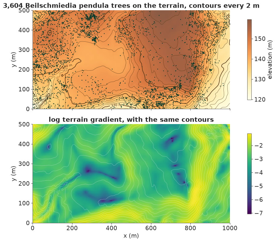
Trees avoid the centre of the plot and bunch into tight clumps. The contours show what that centre is: a flat hollow, with a western rise, a higher plateau to the east and steep edges running between them. Density climbs steadily with gradient, from 20 to 107 trees per hectare across the quarters of the plot. Elevation shows no steady trend: density rises from about 60 to 108 trees per hectare over the first three quarters, then the highest quarter holds the fewest trees of all. That is a first hint that the link to elevation is not the same everywhere. (The R documentation says 3,605 trees; the file holds 3,604.)
For a homogeneous Poisson process, counts across quadrats have variance equal to their mean, whatever the quadrat size. Here:
def vmr(counts, block):
    """Variance-to-mean ratio of counts summed over blocks of `block` x `block` cells."""
    ny, nx = counts.shape
    b = counts.reshape(ny // block, block, nx // block, block).sum((1, 3))
    return b.var() / b.mean()


print(pd.Series({f"{5 * b} m": vmr(y5, b) for b in (1, 2, 4, 10, 20)}, name="variance / mean of counts").round(1).to_string())
5 m       2.1
10 m      4.2
20 m      9.0
50 m     24.1
100 m    51.7
The ratio climbs from 2 at 5 m to 52 at 100 m: clustering at every scale, far more than the terrain alone can produce (a Poisson fit with only the terrain covariates gives about 1 at 5 m and 10-14 at 100 m). This table will be our posterior predictive check in part 9.
The model
Counts in each cell $i$ of area $a$ are Poisson with
$$\log \lambda_i = \alpha + \big(b_e + g_e(s_i)\big)\,\text{elev}_i + \big(b_g + g_g(s_i)\big)\,\text{grad}_i + f_{\text{broad}}(s_i) + f_{\text{fine}}(s_i) + \log a .$$
The fields $g_e$ and $g_g$ are spatially varying effects of elevation and of log gradient (Matern 3/2, sharing one lengthscale), so the species' response to terrain can change across the plot. $f_{\text{broad}}$ is large-scale variation that the terrain does not explain (Matern 3/2). $f_{\text{fine}}$ holds the clumps left by local seed dispersal. It uses a much rougher Matern 1/2 kernel with 100 x 200 modes, reaching about 80% of the lattice's Nyquist frequency.
Each field is a Hilbert-space GP (Solin & Särkkä 2020; as in E05), written non-centred. On a grid the basis factorises, so a field is
$$f = \Phi_y \,\big(\sqrt{S} \circ z\big)\, \Phi_x^\top,$$
two dense matrix products per field per gradient. This is the operation a GPU likes best.
Two choices in the fields matter. With a smoother Matern 3/2 kernel and 64 x 128 modes, the fine
field's lengthscale comes out near 6 m, against a 20 m prior and below what those modes can
resolve. The rougher kernel with more modes fits better, though its lengthscale, about 7 m, stays
close to the 5 m resolution. The basis realises about 75% of the nominal variance of such a field,
so s_fine is a nominal scale and the realised sd is about 0.95.
The smooth fields need room. In a box only 1.25 times the plot's size, the boundary pulls their variance down to about 40% at the north and south edges, and they are no longer stationary. They use a box of half-width 800 m instead, with modes to match, which is why the count reaches 24,810.
Priors. Field sds are LogNormal rather than half-normal. The reason is sampling, not ecology, and part 6 shows why it matters. One consequence to remember: these priors rule out exactly zero variation.
def basis(n, cell, half_width, m):
    """Laplacian eigenfunctions on [-L, L] at `n` cell centres, and their frequencies."""
    centres = (np.arange(n) + 0.5) * cell
    x = centres - centres.mean()
    w = np.pi * np.arange(1, m + 1) / (2 * half_width)
    return np.sqrt(1 / half_width) * np.sin(w[None, :] * (x[:, None] + half_width)), w


def matern_sqrt_density(w2, ell, nu):
    """Square root of the 2-D Matern spectral density, nu = 1/2 or 3/2."""
    constant = {0.5: 2 * np.pi / ell, 1.5: 6 * np.pi * 3**1.5 / ell**3}[nu]
    return pt.sqrt(constant) * ((2 * nu) / ell**2 + w2) ** (-(nu + 1) / 2)


def make_model(cell=CELL, m_fine=M_FINE, m_smooth=M_SMOOTH):
    y, elev, grad, ny, nx = lattice(cell)
    fx = pytensor.config.floatX
    Ly, Lx = 1.25 * 250.0, 1.25 * 500.0
    Py, wy = basis(ny, cell, Ly, m_fine[0])
    Px, wx = basis(nx, cell, Lx, m_fine[1])
    Qy, vy = basis(ny, cell, L_SMOOTH, m_smooth[0])
    Qx, vx = basis(nx, cell, L_SMOOTH, m_smooth[1])
    w2 = (wy[:, None] ** 2 + wx[None, :] ** 2).astype(fx)
    v2 = (vy[:, None] ** 2 + vx[None, :] ** 2).astype(fx)
    Py, Px, Qy, Qx = Py.astype(fx), Px.astype(fx), Qy.astype(fx), Qx.astype(fx)
    elev, grad = elev.astype(fx), grad.astype(fx)
    log_area = np.log(cell**2 / 1e4)  # intensity is per hectare

    with pm.Model() as model:
        alpha = pm.Normal("alpha", np.log(30.0), 1.0)
        b_elev = pm.Normal("b_elev", 0.0, 1.0)
        b_grad = pm.Normal("b_grad", 0.0, 1.0)
        s_broad = pm.LogNormal("s_broad", np.log(0.7), 0.5)
        ell_broad = pm.LogNormal("ell_broad", np.log(120.0), 0.4)
        s_fine = pm.LogNormal("s_fine", np.log(0.7), 0.5)
        ell_fine = pm.LogNormal("ell_fine", np.log(20.0), 0.6)
        s_slope_elev = pm.LogNormal("s_slope_elev", np.log(0.5), 0.5)
        s_slope_grad = pm.LogNormal("s_slope_grad", np.log(0.5), 0.5)
        ell_slope = pm.LogNormal("ell_slope", np.log(200.0), 0.4)
        z_broad = pm.Normal("z_broad", 0.0, 1.0, shape=m_smooth)
        z_fine = pm.Normal("z_fine", 0.0, 1.0, shape=m_fine)
        z_elev = pm.Normal("z_elev", 0.0, 1.0, shape=m_smooth)
        z_grad = pm.Normal("z_grad", 0.0, 1.0, shape=m_smooth)

        smooth = lambda z, sd: Qy @ (sd * z) @ Qx.T
        broad = smooth(z_broad, s_broad * matern_sqrt_density(v2, ell_broad, 1.5))
        fine = Py @ (s_fine * matern_sqrt_density(w2, ell_fine, 0.5) * z_fine) @ Px.T
        sd_slope = matern_sqrt_density(v2, ell_slope, 1.5)
        slope_elev = b_elev + smooth(z_elev, s_slope_elev * sd_slope)
        slope_grad = b_grad + smooth(z_grad, s_slope_grad * sd_slope)
        habitat = alpha + slope_elev * elev + slope_grad * grad + broad
        eta = habitat + fine + log_area
        pm.Poisson("y", pt.exp(eta), observed=y)
    outputs = {"eta": eta, "habitat": habitat, "slope_elev": slope_elev, "slope_grad": slope_grad}
    return model, y, outputs


model, y, outputs = make_model()
print(f"{y.size:,} cells, {sum(v.size for v in model.initial_point().values()):,} parameters")
20,000 cells, 24,810 parameters
A prior predictive check: the total number of trees should cover the observed 3,604 without being dominated by absurd forests.
HYPER = ["alpha", "b_elev", "b_grad", "s_broad", "ell_broad", "s_fine", "ell_fine",
         "s_slope_elev", "s_slope_grad", "ell_slope"]
with model:
    prior = pm.sample_prior_predictive(200, var_names=["y"], random_seed=RANDOM_SEED)
prior_y = prior.prior_predictive["y"].values[0]
total = prior_y.sum((1, 2))
print("prior predictive trees in the plot, 5/50/95%:", np.percentile(total, [5, 50, 95]).round(-2))
print("cells with count above 1,000 in", f"{(prior_y.max((1, 2)) > 1000).mean():.0%} of prior draws")
del prior, prior_y
prior predictive trees in the plot, 5/50/95%: [   900.   9700. 217400.]
cells with count above 1,000 in 14% of prior draws
The prior is generous: a 90% interval of about 900 to 220,000 trees, and 14% of draws put more than 1,000 trees in a single 25 square metre cell. That upper tail is unrealistic, but 20,000 cells of data will overwhelm it, and the observed total sits comfortably inside.
2 · The baseline: NUTS on the CPU
A speed-up is only as honest as its baseline. nutpie is a very good NUTS sampler, so we run it in
double precision on the same model and configure it well, in three ways. First, one BLAS thread
per chain, set at the very top of the notebook. Left alone, each chain's matrix products compete
for a 30-thread pool, and the run is about 2-3x slower for that reason alone. Second, more chains
than the default: 8, one per physical core, sharing 4,000 draws. Third, memory: nutpie stores every
free variable, because var_names only filters derived ones, so the trace goes to a temporary zarr
store on disk, a GB or so, and only the hyperparameters come back.
with precision("float64"):
    model64, _, _ = make_model()
    t0 = time.perf_counter()
    # nutpie stores every free variable (var_names only filters derived ones): the trace goes to disk and only
    # the hyperparameters come back into memory
    with tempfile.TemporaryDirectory() as trace_dir:
        idata_nuts = nutpie.sample(nutpie.compile_pymc_model(model64, var_names=HYPER), draws=NUTS_DRAWS, tune=400,
                                   chains=NUTS_CHAINS, cores=NUTS_CHAINS, seed=RANDOM_SEED, progress_bar=False,
                                   save_warmup=False, store_mass_matrix=False,
                                   zarr_store=nutpie.zarr_store.LocalStore(trace_dir))
        nuts_wall = time.perf_counter() - t0
        draws_nuts = np.stack([idata_nuts.posterior[n].values for n in HYPER], -1)
        n_steps = float(idata_nuts.sample_stats["n_steps"].mean())
        diverging = int(idata_nuts.sample_stats["diverging"].sum())
    del model64, idata_nuts
tuning = 400

ds_nuts = xr.Dataset({n: (("chain", "draw"), draws_nuts[..., i]) for i, n in enumerate(HYPER)})
rhat_nuts, ess_nuts = az.rhat(ds_nuts), az.ess(ds_nuts)
summary_nuts = pd.DataFrame({"mean": draws_nuts.mean((0, 1)), "sd": draws_nuts.std((0, 1)),
                             "r_hat": [float(rhat_nuts[n]) for n in HYPER],
                             "ess": [float(ess_nuts[n]) for n in HYPER]}, index=HYPER)
print(f"nutpie on the CPU: {NUTS_CHAINS} chains, {nuts_wall:.0f} s, {diverging} divergences, {n_steps:.0f} leapfrog steps per draw, {tuning} tuning steps")
print(summary_nuts.round(3).to_string())
nutpie on the CPU: 8 chains, 121 s, 0 divergences, 63 leapfrog steps per draw, 400 tuning steps
                 mean      sd  r_hat       ess
alpha           3.412   0.375  1.031   231.645
b_elev          0.613   0.342  1.037   268.006
b_grad          0.534   0.250  1.028   344.495
s_broad         1.091   0.190  1.036   320.751
ell_broad     112.076  26.022  1.055   136.325
s_fine          1.103   0.036  1.005  1460.784
ell_fine        7.014   0.788  1.014   770.687
s_slope_elev    0.779   0.243  1.034   292.868
s_slope_grad    0.554   0.170  1.009   654.378
ell_slope     164.480  47.197  1.022   442.345
It works: about 120 s, no divergences, and only about 63 leapfrog steps per draw, because the
non-centred posterior is well conditioned. The weakness is effective sample size. The worst
parameter, ell_broad, reaches an ESS of only about 140 with r_hat 1.05, the usual trouble with
the hyperparameters of a latent Gaussian model. Are 8 chains too few? A separate run with 14
chains took 139 s and reached a worst ESS of 187 with r_hat 1.10: about 20% more ESS per second,
so the choice of 8 hides little.
3 · Where the time goes: chains, problem size and precision
Now JAX starts. get_jaxified_logp turns the PyMC model into a JAX function, so the model stays
in PyMC. Beware of its flag: negative_logp=True, the default, returns +logp, and False
flips the sign. We check it against PyMC on a small lattice, because compile_logp is
memory-hungry at full size.
We time value_and_grad under vmap, the unit of all gradient-based sampling. block_until_ready
matters: JAX dispatches work asynchronously, and without it we would time the queueing rather than
the arithmetic.
import blackjax  # CUDA starts here, not before
import optax
from blackjax.adaptation.base import get_filter_adapt_info_fn

key = jax.random.key(RANDOM_SEED)
if (jax.default_backend() == "gpu") != HAS_GPU:
    raise RuntimeError(f"expected GPU={HAS_GPU} but JAX chose {jax.default_backend()}: if your GPU is not usable, "
                       "run with JAX_PLATFORMS=cpu")
print("JAX backend:", jax.default_backend(), jax.devices())


def jaxify(m):
    """One flat parameter vector -> log density, plus the unravel function."""
    logp = get_jaxified_logp(m)  # NB: the default negative_logp=True returns +logp
    start = m.initial_point()
    names = [v.name for v in m.value_vars]
    q0, unravel = ravel_pytree([jnp.asarray(start[n]) for n in names])
    return (lambda q: logp(unravel(q))), q0, unravel, names


logdensity, q0, unravel, names = jaxify(model)
print("value variables:", names[:10], "...")
small, _, _ = make_model(25.0, (20, 40), (16, 16))  # the check on a small lattice: compile_logp is heavy
f_small, q_small, _, _ = jaxify(small)
print(f"25 m lattice: PyMC logp {small.compile_logp()(small.initial_point()):.2f}, JAX logp {float(f_small(q_small)):.2f}")
del small, f_small, q_small
NH = len(HYPER)
value_is_log = np.array([n.endswith("_log__") for n in names[:NH]])


def timed(fn, *args, repeat=5):
    """(compile seconds, best-of-`repeat` run seconds). block_until_ready defeats async dispatch."""
    t0 = time.perf_counter()
    jax.block_until_ready(fn(*args))
    compile_s = time.perf_counter() - t0
    runs = []
    for _ in range(repeat):
        t0 = time.perf_counter()
        jax.block_until_ready(fn(*args))
        runs.append(time.perf_counter() - t0)
    return compile_s, min(runs)


def batch_gradient(f, q, chains, device):
    Q = jax.device_put(q + 0.1 * jnp.asarray(rng.normal(size=(chains, q.size)), q.dtype), device)
    result = timed(jax.jit(jax.vmap(jax.value_and_grad(f))), Q)
    jax.clear_caches()  # every chain count is a new compiled program, kept alive otherwise
    return result


cpu = jax.devices("cpu")[0]
gpu = jax.devices("gpu")[0] if HAS_GPU else None
chain_grid = sorted({1, 8, 32, 128, 512, CHAINS}) if HAS_GPU else sorted({1, 8, CHAINS})
rows = []
for chains in chain_grid:
    compile_cpu, cpu_s = batch_gradient(logdensity, q0, chains, cpu) if chains <= 128 else (np.nan, np.nan)
    row = {"chains": chains, "CPU float32": cpu_s * 1e3, "compile CPU s": compile_cpu}
    if HAS_GPU:
        compile_gpu, gpu_s = batch_gradient(logdensity, q0, chains, gpu)
        row |= {"GPU float32": gpu_s * 1e3, "compile GPU s": compile_gpu}
    rows.append(row)
timing = pd.DataFrame(rows).set_index("chains")

if HAS_GPU:  # the same model in double precision
    with precision("float64"):
        model64, _, _ = make_model()
        f64, q64, _, _ = jaxify(model64)
        timing["GPU float64"] = [batch_gradient(f64, q64, c, gpu)[1] * 1e3 for c in chain_grid]
    del model64, f64, q64
    timing["GPU speed-up"] = timing["CPU float32"] / timing["GPU float32"]
    timing["float32 speed-up on GPU"] = timing["GPU float64"] / timing["GPU float32"]
print(timing.round(2).to_string())
JAX backend: gpu [CudaDevice(id=0)]
value variables: ['alpha', 'b_elev', 'b_grad', 's_broad_log__', 'ell_broad_log__', 's_fine_log__', 'ell_fine_log__', 's_slope_elev_log__', 's_slope_grad_log__', 'ell_slope_log__'] ...
25 m lattice: PyMC logp -6321.62, JAX logp -6321.62
        CPU float32  compile CPU s  GPU float32  compile GPU s  GPU float64  GPU speed-up  float32 speed-up on GPU
chains
1              0.71           0.39         0.13           1.88         0.34          5.41                     2.59
8              2.25           0.39         0.18           1.92         1.13         12.71                     6.40
32             5.62           0.42         0.34           2.19         3.95         16.72                    11.75
128           44.73           0.46         0.85           2.00        14.34         52.80                    16.93
512             NaN            NaN         2.95           2.13        50.50           NaN                    17.11
Read the table in three directions.
Down the columns: chains. On the GPU, cost grows slowly at first: 128 chains cost about 6.5 times what one chain costs, not 128 times. The GPU's advantage grows from about 5x with one chain to more than 50x with 128. The CPU, with a fixed number of cores, falls behind: from 32 to 128 chains its time rises about eightfold, not fourfold, which suggests the work no longer fits in cache.
Across: precision. This is the surprise, and it is specific to consumer cards. The double-precision hardware on this GPU is a small fraction of its single-precision hardware, so float32 is about 17x faster at 128 chains. On this card float64 alone would throw away most of the GPU's gain. Data-centre GPUs do not have this penalty.
Compile time goes the other way: about 2 s on the GPU against 0.4 s on the CPU. That is negligible here, but it would dominate a workflow that recompiles for thousands of small fits.
Next, what happens as the problem shrinks?
sizes = []
if HAS_GPU:
    for cell, mf, ms in ((25.0, (20, 40), (16, 16)), (20.0, (25, 50), (20, 20)), (10.0, (50, 100), (30, 30)), (5.0, M_FINE, M_SMOOTH)):
        m_, y_, _ = make_model(cell, mf, ms)
        f_, q_, _, _ = jaxify(m_)
        for chains in (1, 128):
            sizes.append({"cell m": cell, "cells": y_.size, "parameters": q_.size, "chains": chains,
                          "cpu ms": batch_gradient(f_, q_, chains, cpu)[1] * 1e3,
                          "gpu ms": batch_gradient(f_, q_, chains, gpu)[1] * 1e3})
        del m_, f_, q_
    sizes = pd.DataFrame(sizes)
    sizes["speed-up"] = sizes["cpu ms"] / sizes["gpu ms"]
    print(sizes.round(2).to_string(index=False))

fig, axes = plt.subplots(1, 2 if HAS_GPU else 1, figsize=(11 if HAS_GPU else 5.5, 4), layout="constrained", squeeze=False)
axes = axes[0]
per_chain = timing.filter(regex="(CPU|GPU) float").div(timing.index, axis=0).dropna(how="all")
for label in per_chain:
    axes[0].plot(per_chain.index, per_chain[label], "o-", label=label)
axes[0].set(xscale="log", yscale="log", xlabel="chains", ylabel="ms per chain per gradient", title="More chains: cheaper per chain")
axes[0].legend(loc="lower left")
if HAS_GPU:
    for chains, group in sizes.groupby("chains"):
        axes[1].plot(group["parameters"], group["speed-up"], "o-", label=f"{chains} chain(s)")
    axes[1].axhline(1, color="k", lw=1, ls=":")
    axes[1].set(xscale="log", yscale="log", xlabel="parameters", ylabel="CPU time / GPU time", title="Bigger problems: larger GPU advantage")
    axes[1].legend();
 cell m  cells  parameters  chains  cpu ms  gpu ms  speed-up
   25.0    800        1578       1    0.07    0.11      0.61
   25.0    800        1578     128    2.19    0.14     15.10
   20.0   1250        2460       1    0.09    0.12      0.79
   20.0   1250        2460     128    2.40    0.19     12.98
   10.0   5000        7710       1    0.21    0.12      1.72
   10.0   5000        7710     128    7.19    0.33     21.52
    5.0  20000       24810       1    0.74    0.13      5.79
    5.0  20000       24810     128   45.99    0.85     54.09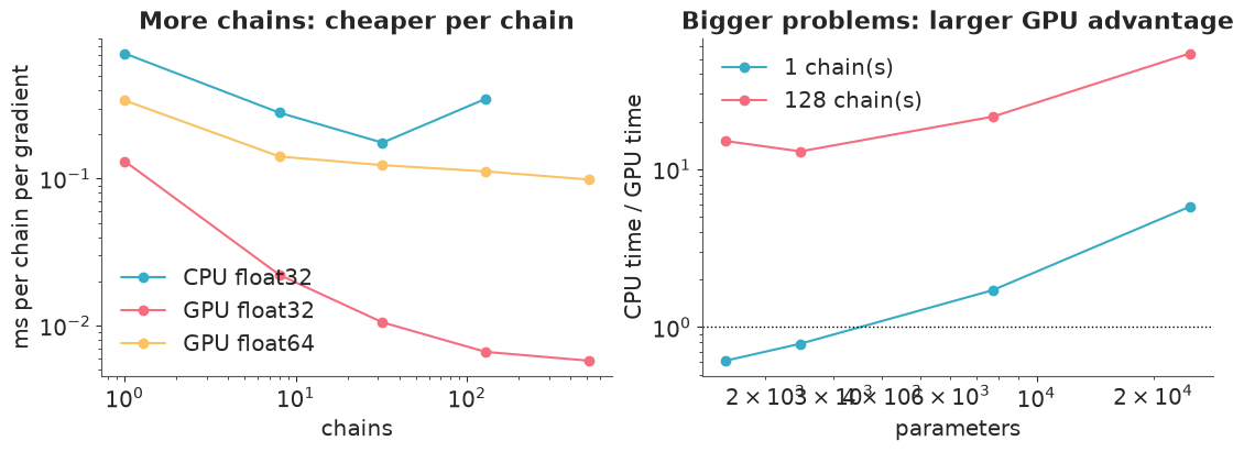
The left panel shows the cost per chain falling as chains are added on the GPU, and the right panel gives the decision rule. The GPU does not help a small problem with one chain: at 1,578 parameters it runs at 0.6x the CPU's speed here (0.5-0.8x across runs), probably because every call pays a fixed cost to reach the card. With 128 chains it wins at every size, by 13x to 54x, and by more as the problem grows. So a GPU is not simply faster. It is faster at large batches of large array operations.
4 · ChEES-HMC: two ways to fail, and a fix
HMC has two settings, step size and trajectory length. NUTS picks the length separately for each
chain at each iteration. ChEES (Hoffman, Radul & Sountsov 2021) instead picks one length for all
chains during warmup, by maximising the Change in the Estimator of the Expected Square: how much
a trajectory moves each chain's squared distance from the ensemble mean. Every chain then runs the
same number of leapfrog steps, jittered from one iteration to the next, so no chain waits for
another. The L printed below is the maximum: each iteration draws a count that averages about L/2.
All chains start from dispersed points, so that r_hat can detect problems. With the default settings, this happens:
key, init_key = jax.random.split(key)
spread = jnp.concatenate([jnp.full(NH, 0.3), jnp.ones(q0.size - NH)]).astype(q0.dtype)
cold_start = q0 + spread * jax.random.normal(init_key, (CHAINS, q0.size), q0.dtype)


def summarise(draws):
    """Posterior summary of hyperparameters, draws of shape (chain, draw, NH) on the value scale."""
    d = np.asarray(draws, float).copy()
    d[..., value_is_log] = np.exp(d[..., value_is_log])
    ds = xr.Dataset({n: (("chain", "draw"), d[..., i]) for i, n in enumerate(HYPER)})
    rhat, ess = az.rhat(ds), az.ess(ds)
    return pd.DataFrame({"mean": d.mean((0, 1)), "sd": d.std((0, 1)),
                         "r_hat": [float(rhat[n]) for n in HYPER],
                         "ess": [float(ess[n]) for n in HYPER]}, index=HYPER)


def sample(step, state, k, snaps, keep, thin):
    """Run the vectorised kernel; every `thin` steps keep hyperparameters, every `keep * thin` all of q."""
    def one(s, ki):
        s, info = jax.vmap(step)(jax.random.split(ki, CHAINS), s)
        steps = jnp.mean(getattr(info, "num_integration_steps", jnp.ones(())))
        return s, (info.acceptance_rate, info.is_divergent, steps)

    def keep_block(s, ki):
        s, (acc, div, steps) = jax.lax.scan(one, s, jax.random.split(ki, thin))
        return s, (s.position[:, :NH], acc.mean(), div.sum(), steps.sum())

    def snap_block(s, ki):
        s, out = jax.lax.scan(keep_block, s, jax.random.split(ki, keep))
        return s, (s.position, out)

    state, (positions, (kept, acc, div, steps)) = jax.lax.scan(snap_block, state, jax.random.split(k, snaps))
    kept = np.asarray(kept).reshape(snaps * keep, CHAINS, NH).transpose(1, 0, 2)
    return state, positions, kept, {"acceptance": float(acc.mean()), "divergences": int(div.sum()),
                                    "gradients per chain": float(steps.sum())}


def warm_chees(k, start, steps, **options):
    warmup = blackjax.chees_adaptation(logdensity, CHAINS, adaptation_info_fn=get_filter_adapt_info_fn(), **options)
    (state, params), _ = warmup.run(k, start, step_size=0.01, optim=optax.adam(0.05), num_steps=steps)
    return jax.block_until_ready(state), params


def run_chees(k, start, **options):
    """Plain ChEES: one warmup, then sampling."""
    k1, k2 = jax.random.split(k)
    t0 = time.perf_counter()
    state, params = warm_chees(k1, start, WARMUP, **options)
    t1 = time.perf_counter()
    state, positions, kept, stats = sample(blackjax.dynamic_hmc(logdensity, **params).step, state, k2, SNAPS, KEEP, 1)
    jax.block_until_ready(positions)
    t2 = time.perf_counter()
    stats |= {"step size": float(params["step_size"]), "L": float(params["integration_steps_params"][0]),
              "warmup s": t1 - t0, "sampling s": t2 - t1}
    return state, params, positions, kept, stats


key, k = jax.random.split(key)
_, _, positions, kept_id, stats_id = run_chees(k, cold_start)
del positions
summary_id = summarise(kept_id)
print({a: round(b, 4) for a, b in stats_id.items()})
print(summary_id.round(3).to_string())
{'acceptance': 0.8894, 'divergences': 1, 'gradients per chain': 23073.0, 'step size': 0.0101, 'L': 153.2255, 'warmup s': 27.7556, 'sampling s': 21.5041}
                 mean      sd  r_hat       ess
alpha           3.404   0.368  1.013  7700.653
b_elev          0.626   0.345  1.014  8493.493
b_grad          0.514   0.245  1.012  9158.615
s_broad         1.100   0.200  1.013  8208.039
ell_broad     114.739  28.097  1.063  1513.397
s_fine          1.104   0.036  1.018  5770.107
ell_fine        7.065   0.815  1.047  2187.840
s_slope_elev    0.785   0.243  1.041  2391.765
s_slope_grad    0.559   0.170  1.033  2735.062
ell_slope     165.009  45.175  1.041  2524.059
Failure 1: no metric. At first sight the run is healthy: acceptance is about 0.89 and there is one divergence (identical runs give anything from none to a few hundred). But the largest r_hat, 1.06, is well above the 1.01 we want, and the worst ESS, about 1,500, is roughly seven times lower than after the fix below (six to twenty times across runs). With the default identity metric nothing corrects for the different scales of the parameters, so the step size stays small, near 0.010.
The fix is mass_matrix_estimation="diagonal", which estimates a diagonal metric from the ensemble
and adds a floor on the trajectory length. The floor needs a d x d covariance accumulator: 2.3 GB
of GPU memory in float32 at this size, and 4.6 GB in float64.
Failure 2: one straggler. With the metric on, most seeds are fine, but not all. Over complete runs with different seeds, the maximum trajectory length came out at 181, 246, 265, 661 and 728 steps, and the high values went with bad results: the run at 728 had 452 divergences and an expected total of 4,428 trees, against 3,604 observed. The cause is a chain that gets stuck early. Its log density sits hundreds of robust sds from the rest, and the floor scales with the spread of the ensemble, so one straggler can inflate the trajectory for every chain. In a test of four seeds, two had stragglers after 300 warmup steps, with lengths of 885 and 978, against 473 and 545 for the other two.
The fix is to warm up in two stages: flag chains far from the ensemble, restart them from copies of healthy ones, then run a second, fresh warmup. With it, all four seeds settled at 105-115 steps. The restart does part of the work by itself, because blackjax starts its adaptation again. Copies separate at once, because their momenta differ, and all of this happens only during warmup, so the target distribution is untouched. The risk is real, though: culling would hide a true minor mode. In the seeds with stragglers, the flagged chains had far lower log density than the rest, so they were stuck rather than exploring. Check that before you reuse this recipe.
log_density_batch = jax.jit(jax.vmap(logdensity))


def stragglers(state, threshold=6.0):
    """Chains more than `threshold` robust sds from the ensemble in log density or any hyperparameter."""
    h = np.c_[np.asarray(log_density_batch(state.position)), np.asarray(state.position[:, :NH])]
    median = np.median(h, 0)
    z = np.abs(h - median) / (1.4826 * np.median(np.abs(h - median), 0))
    return (z > threshold).any(1), z


def cull(state, bad):
    """Warmup only: restart flagged chains from copies of healthy ones (their paths separate at once)."""
    source = np.arange(CHAINS)
    source[bad] = rng.choice(np.flatnonzero(~bad), bad.sum())
    return jax.tree.map(lambda leaf: leaf[source], state)


key, k1, k2, k3 = jax.random.split(key, 4)
options = {"mass_matrix_estimation": "diagonal"}
t0 = time.perf_counter()
state, params = warm_chees(k1, cold_start, int(0.3 * WARMUP), **options)
bad, z = stragglers(state)
print(f"stage 1 ({int(0.3 * WARMUP)} steps): step size {float(params['step_size']):.4f}, L = {float(params['integration_steps_params'][0]):.0f}, {bad.sum()} straggler(s); "
      f"worst log density z = {z[:, 0].max():.1f}; stragglers' log density {np.asarray(log_density_batch(state.position))[bad].round(0)}, "
      f"median {np.median(np.asarray(log_density_batch(state.position))):.0f}")
state = cull(state, bad)
state, params_chees = warm_chees(k2, state.position, WARMUP - int(0.3 * WARMUP), **options)
bad, z = stragglers(state)
print(f"stage 2 ({WARMUP - int(0.3 * WARMUP)} steps): step size {float(params_chees['step_size']):.4f}, L = {float(params_chees['integration_steps_params'][0]):.0f}, {bad.sum()} straggler(s) culled")
state = cull(state, bad)
t1 = time.perf_counter()
state_chees, pos_chees, kept_chees, stats_chees = sample(blackjax.dynamic_hmc(logdensity, **params_chees).step, state, k3, SNAPS, KEEP, 1)
jax.block_until_ready(pos_chees)
stats_chees |= {"step size": float(params_chees["step_size"]), "L": float(params_chees["integration_steps_params"][0]),
                "warmup s": t1 - t0, "sampling s": time.perf_counter() - t1}
summary_chees = summarise(kept_chees)
print({a: round(b, 4) for a, b in stats_chees.items()})
print(summary_chees.round(3).to_string())

fig, axes = plt.subplots(1, 2, figsize=(10, 3.6), sharex=True, sharey=True, layout="constrained")
i = HYPER.index("s_fine")
means = [np.exp(kept[..., i]).mean(1) for kept in (kept_id, kept_chees)]
bins = np.linspace(min(m.min() for m in means), max(m.max() for m in means), 40)
for ax, m, title in zip(axes, means, ("ChEES, default settings", "ChEES, diagonal metric + floor")):
    ax.hist(m, bins=bins, color="C0")
    ax.set(title=title, xlabel="per-chain mean of s_fine")
axes[0].set_ylabel("chains");
stage 1 (300 steps): step size 0.0213, L = 606, 0 straggler(s); worst log density z = 2.7; stragglers' log density [], median -42347
stage 2 (700 steps): step size 0.0262, L = 180, 0 straggler(s) culled
{'acceptance': 0.8983, 'divergences': 2, 'gradients per chain': 27161.0, 'step size': 0.0262, 'L': 179.9161, 'warmup s': 112.9551, 'sampling s': 24.6254}
                 mean      sd  r_hat        ess
alpha           3.398   0.371  1.005  30698.661
b_elev          0.617   0.343  1.004  31183.001
b_grad          0.510   0.248  1.006  30839.353
s_broad         1.102   0.203  1.004  22690.534
ell_broad     114.256  28.052  1.009  10210.765
s_fine          1.104   0.036  1.005  16416.239
ell_fine        7.069   0.810  1.008  11046.686
s_slope_elev    0.781   0.241  1.004  17539.094
s_slope_grad    0.557   0.171  1.005  17063.921
ell_slope     165.953  45.763  1.006  14452.420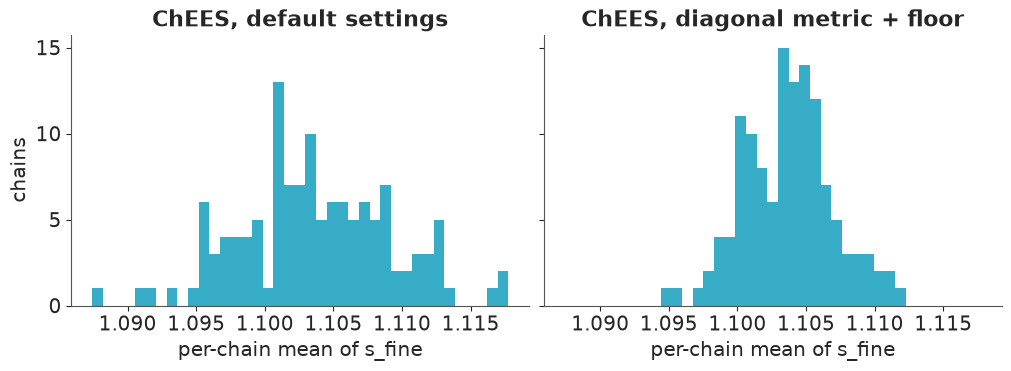
This seed has no stragglers, though the check stays, because nobody can know that in advance. Notice that L still falls from about 600 to 180 with nothing culled: a high early L alone is not proof of a straggler, and the second warmup does that work. The run has 2 divergences, r_hat at most 1.01 and a worst ESS of about 10,000 (8,000-10,000 across runs), some seventy-five times nutpie's, in about 140 s. Warmup takes over 80% of that time. In the figure, the default run's chains are spread more widely than the fixed run's, which is what a high r_hat looks like.
5 · Why not just run NUTS on the GPU?
The usual explanation is that NUTS trees differ between chains, so under vmap every chain waits
for the largest tree. Let us measure that, on the same model with the same metric and step size.
steps_nuts = 30 if HAS_GPU else 10
nuts = blackjax.nuts(logdensity, step_size=params_chees["step_size"], inverse_mass_matrix=params_chees["inverse_mass_matrix"])
nuts_state = jax.vmap(nuts.init)(state_chees.position)


def nuts_iteration(s, ki):
    s, info = jax.vmap(nuts.step)(jax.random.split(ki, CHAINS), s)
    return s, info.num_integration_steps


nuts_run = jax.jit(lambda k: jax.lax.scan(nuts_iteration, nuts_state, jax.random.split(k, steps_nuts))[1])
key, k = jax.random.split(key)
tree_sizes = np.asarray(jax.block_until_ready(nuts_run(k)))   # compiles
key, k = jax.random.split(key)
t0 = time.perf_counter()
tree_sizes = np.asarray(jax.block_until_ready(nuts_run(k)))
nuts_s = time.perf_counter() - t0

chees_step = blackjax.dynamic_hmc(logdensity, **params_chees).step


def chees_iteration(s, ki):
    s, info = jax.vmap(chees_step)(jax.random.split(ki, CHAINS), s)
    return s, (info.num_integration_steps, s.position.mean())  # the sizes alone are a fixed sequence: without
    #                                                             the position XLA deletes the whole sampler


chees_run = jax.jit(lambda k: jax.lax.scan(chees_iteration, state_chees, jax.random.split(k, steps_nuts))[1])
key, k = jax.random.split(key)
jax.block_until_ready(chees_run(k))
key, k = jax.random.split(key)
t0 = time.perf_counter()
chees_sizes = np.asarray(jax.block_until_ready(chees_run(k))[0])
chees_s = time.perf_counter() - t0
bare = timing.loc[CHAINS, "GPU float32" if HAS_GPU else "CPU float32"]
print(f"vectorised NUTS: {tree_sizes.mean():.0f} leapfrog steps per iteration, largest tree per iteration {tree_sizes.max(1).mean():.0f}; "
      f"tree sizes seen {np.unique(tree_sizes)}; {tree_sizes.sum() / (tree_sizes.max(1).sum() * CHAINS):.0%} of the work needed")
print(pd.DataFrame({"gradients per iteration": [tree_sizes.max(1).mean(), chees_sizes.max(1).mean()],
                    "ms per gradient": [1e3 * nuts_s / tree_sizes.max(1).sum(), 1e3 * chees_s / chees_sizes.max(1).sum()]},
                   index=["NUTS", "ChEES"]).round(2).to_string())
print(f"a bare batched gradient costs {bare:.2f} ms")
del nuts_run, chees_run
jax.clear_caches()
vectorised NUTS: 127 leapfrog steps per iteration, largest tree per iteration 127; tree sizes seen [ 38 127]; 100% of the work needed
       gradients per iteration  ms per gradient
NUTS                    127.00             3.59
ChEES                    92.17             0.86
a bare batched gradient costs 0.85 ms
The usual explanation does not apply here. Almost every tree has 127 steps, with the odd smaller one, so no work is wasted: this posterior is so homogeneous that the chains stop at the same depth. On a model with more varied geometry the trees would differ, and that cost would appear.
The cost that does appear is bookkeeping. Each NUTS gradient costs about 3.6 ms, against
0.86 ms for ChEES, which matches a bare batched gradient. Building trees under vmap means saving
and masking states, and while_loops that XLA cannot flatten. ChEES has almost no overhead: its
time is its gradients.
The benchmark has a trap of its own. num_integration_steps is a fixed sequence, so timing it
alone lets XLA delete the entire sampler as dead code. We return a statistic of the positions to
keep the work alive.
6 · MEADS: fragile from a cold start, excellent from a warm one
MEADS (Hoffman & Sountsov 2022) goes further and removes the trajectory altogether. It uses generalised HMC: a single leapfrog step per iteration, with momentum kept and only partly refreshed. During warmup the chains are split into folds. Each fold takes its step size and metric from a neighbouring fold and its damping from its own positions, one fold is frozen at each step, and the chains are reshuffled. Sampling then uses one fixed kernel with averaged settings. There is no trajectory length to tune, and no warmup optimiser.
Start it from the same dispersed points:
def run_meads(k, start, multiplier):
    k1, k2 = jax.random.split(k)
    t0 = time.perf_counter()
    warmup = blackjax.meads_adaptation(logdensity, CHAINS, num_folds=4, step_size_multiplier=multiplier,
                                       adaptation_info_fn=get_filter_adapt_info_fn())
    (state, params), _ = warmup.run(k1, start, MEADS_WARMUP)
    jax.block_until_ready(state)
    t1 = time.perf_counter()
    state, positions, kept, stats = sample(blackjax.ghmc(logdensity, **params).step, state, k2, SNAPS, MEADS_KEEP, MEADS_THIN)
    jax.block_until_ready(positions)
    t2 = time.perf_counter()
    scale = np.asarray(params["momentum_inverse_scale"])
    stats |= {"step size": float(params["step_size"]), "alpha": float(params["alpha"]), "delta": float(params["delta"]),
              "largest scale": float(scale.max()), "warmup s": t1 - t0, "sampling s": t2 - t1}
    return state, params, positions, kept, stats


key, k = jax.random.split(key)
_, _, positions, kept_cold, stats_cold = run_meads(k, cold_start, 0.25)
del positions
print("MEADS, cold start:", {a: round(b, 5) for a, b in stats_cold.items()})
print(summarise(kept_cold)[["r_hat", "ess"]].round(2).T.to_string())
MEADS, cold start: {'acceptance': 0.82452, 'divergences': 0, 'gradients per chain': 39000.0, 'step size': 0.0, 'alpha': 0.0001, 'delta': 5e-05, 'largest scale': 15.30351, 'warmup s': 39.11603, 'sampling s': 46.62223}
        alpha  b_elev  b_grad  s_broad  ell_broad  s_fine  ell_fine  s_slope_elev  s_slope_grad  ell_slope
r_hat  118.23   82.51   43.56    29.89     186.84   15.26     41.89         32.91         26.95      31.35
ess    130.02  130.11  130.07   130.15     130.01  130.58    130.08        130.13        130.20     130.15
Failure 3: a clean-looking catastrophe. Acceptance is about 0.8 and there are no divergences, yet r_hat runs from 15 to nearly 190, and ESS equals the number of chains. The step size has collapsed to zero, so the chains are frozen, and a frozen chain accepts its proposals. MEADS sets the step size from an estimate of the largest eigenvalue of the scaled gradients, and from a dispersed start one chain with a huge gradient can dominate that estimate.
A short Adam optimisation beforehand does not help. In an earlier run it overshot the typical set to a mode with log density near -23,000, where posterior draws sat near -37,700 in that run, and gradients in that funnel are larger still. What helps is a start in the typical set, which ChEES has already given us.
Three more settings matter. The first is step_size_multiplier=0.25: the default of 0.5 gives
acceptance of only 0.15-0.4 and r_hat from 1.2 to 2. The second is enough chains in each fold. On
the 20 m lattice, 32 chains (8 per fold) collapsed on one seed of three, while 64 chains (16 per
fold) held on all three, which is why the CPU configuration uses 64.
The third is the priors, and it is the instructive one. With half-normal and then Gamma priors on the field sds, MEADS blew up: a log-sd ran to about -44 million. float32 is the obvious suspect, since GHMC's one-step Metropolis test compares tiny energy differences, but the blow-up happens in float64 too. (float32 does bring far more divergences, 1,266 against 3 in one comparison, but rounding of this size cannot cause a divergence by itself, and the mechanism remains unknown.) The most likely reading is this: those priors have a linear tail in log sd, with a nearly constant gradient, so nothing limits the step in that direction. A chain wanders down the tail, the fold's scale estimate grows, and that makes the next step bigger. A LogNormal prior has a quadratic tail, whose gradient grows with distance. With it, MEADS converged on all three seeds tried at 128 chains.
key, k = jax.random.split(key)
_, params_meads, pos_meads, kept_meads, stats_meads = run_meads(k, state_chees.position, 0.25)
summary_meads = summarise(kept_meads)
print("MEADS, started from ChEES:", {a: round(b, 5) for a, b in stats_meads.items()})
print(summary_meads.round(3).to_string())
MEADS, started from ChEES: {'acceptance': 0.97654, 'divergences': 0, 'gradients per chain': 39000.0, 'step size': 0.016, 'alpha': 0.00617, 'delta': 0.00309, 'largest scale': 1.47273, 'warmup s': 31.96501, 'sampling s': 46.14637}
                 mean      sd  r_hat        ess
alpha           3.398   0.365  1.006  19962.562
b_elev          0.617   0.338  1.006  22825.406
b_grad          0.511   0.248  1.005  19914.657
s_broad         1.098   0.201  1.004  21491.688
ell_broad     113.541  27.718  1.011  10166.427
s_fine          1.102   0.037  1.007  14622.563
ell_fine        7.065   0.814  1.008  11803.045
s_slope_elev    0.776   0.241  1.005  15511.039
s_slope_grad    0.554   0.167  1.004  19062.212
ell_slope     166.002  45.878  1.006  16273.271
From a clean ensemble, MEADS is excellent: acceptance 0.98, no divergences, r_hat at most 1.01 and a worst ESS of about 10,000. It varies between identical runs (acceptance 0.94-0.98, worst ESS 10,000-19,000). Its step size is small, 0.016 here and up to 0.03 in other runs, and so is its damping, so momentum persists for a hundred steps or more: long trajectories, built one step at a time.
7 · The scorecard, and how much of it is the hardware
where = "GPU" if HAS_GPU else "CPU"
order = pd.DataFrame({
    f"ChEES ({where})": [stats_chees["warmup s"] + stats_chees["sampling s"], summary_chees.ess.min(), summary_chees.r_hat.max(), stats_chees["divergences"]],
    f"MEADS after ChEES ({where})": [stats_chees["warmup s"] + stats_chees["sampling s"] + stats_meads["warmup s"] + stats_meads["sampling s"], summary_meads.ess.min(), summary_meads.r_hat.max(), stats_meads["divergences"]],
    "NUTS, nutpie (CPU)": [nuts_wall, summary_nuts.ess.min(), summary_nuts.r_hat.max(), diverging],
}, index=["seconds", "worst ESS", "worst r_hat", "divergences"]).T
if HAS_GPU and CHAINS % 32 == 0 and np.isfinite(timing.loc[CHAINS, "CPU float32"]):
    # Same ESS, total GPU time scaled by a measured gradient-time ratio: estimates, not runs.
    gpu_ms = timing.loc[CHAINS, "GPU float32"]
    for label, cpu_ms in ((f"ChEES (CPU, one {CHAINS}-chain batch, estimated)", timing.loc[CHAINS, "CPU float32"]),
                          ("ChEES (CPU, 32-chain batches, estimated)", timing.loc[32, "CPU float32"] * CHAINS / 32)):
        order.loc[label] = order.loc[f"ChEES ({where})"]
        order.loc[label, "seconds"] *= cpu_ms / gpu_ms
order["worst ESS per second"] = order["worst ESS"] / order["seconds"]
order["ESS/s vs NUTS"] = order["worst ESS per second"] / order.loc["NUTS, nutpie (CPU)", "worst ESS per second"]
print(order.round(2).to_string())

fig, axes = plt.subplots(2, 5, figsize=(12, 4.8), layout="constrained")
for ax, name in zip(axes.flat, HYPER):
    for row, (label, s) in enumerate((("ChEES", summary_chees), ("MEADS", summary_meads), ("NUTS", summary_nuts))):
        ax.errorbar(s.loc[name, "mean"], row, xerr=s.loc[name, "sd"], fmt="o", color=f"C{row}")
    ax.set(title=name, yticks=[0, 1, 2], yticklabels=["ChEES", "MEADS", "NUTS"], ylim=(-0.6, 2.6))
    ax.locator_params(axis="x", nbins=4);
                                             seconds  worst ESS  worst r_hat  divergences  worst ESS per second  ESS/s vs NUTS
ChEES (GPU)                                   137.58   10210.76         1.01          2.0                 74.22          66.09
MEADS after ChEES (GPU)                       215.69   10166.43         1.01          0.0                 47.13          41.97
NUTS, nutpie (CPU)                            121.40     136.33         1.05          0.0                  1.12           1.00
ChEES (CPU, one 128-chain batch, estimated)  7264.12   10210.76         1.01          2.0                  1.41           1.25
ChEES (CPU, 32-chain batches, estimated)     3653.80   10210.76         1.01          2.0                  2.79           2.49
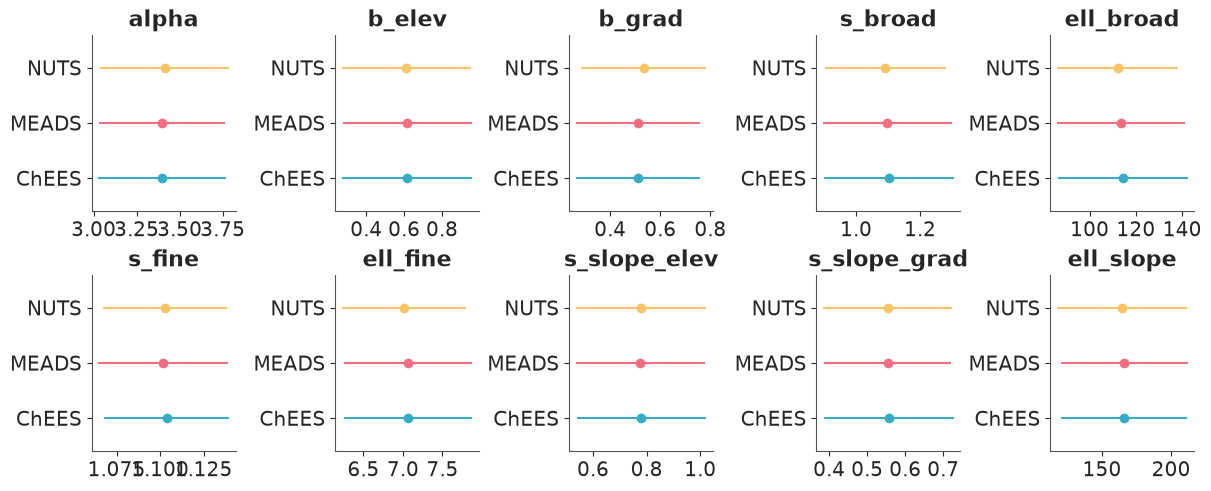
All three samplers agree on all ten hyperparameters, although ChEES and MEADS ran in float32 on a GPU and nutpie in float64 on a CPU. That independent agreement is what lets us trust the speed-up. In worst-case ESS per second, ChEES is about 65x NUTS in this run and MEADS about 40x (55-70x and 40-50x across runs). With 14 chains for nutpie, as measured in part 2, both would fall by about a fifth.
The baseline is half the story. Let nutpie's chains fight over a BLAS thread pool and give it only 4 chains, and the same GPU runs look about 200x faster. Nothing about the GPU changes.
Nor is the speed-up the GPU alone. The last two rows separate the effects. They scale ChEES's total time by a measured ratio of gradient times, so they are estimates, not runs. As one 128-chain batch on the CPU, ChEES would take about two hours and roughly match NUTS. In 32-chain batches, the CPU's better regime, it would take about an hour and reach about 2.5x NUTS, assuming ESS and adaptation hold. So the hardware gives roughly 25-30x and the algorithm roughly 2-2.5x. The two depend on each other: the GPU's advantage exists only because the algorithm can run 128 chains in lock-step. On the 20 m lattice, measured on 8 CPU cores without a GPU, nutpie simply wins: ChEES reaches about 0.75x and MEADS about 0.5x of its ESS per second. (MEADS's time includes the whole ChEES run it starts from.)
Two limits apply. The worst ESS is taken over ten hyperparameters, and says nothing about multimodal posteriors, where every ensemble method can agree confidently on the wrong answer. And ESS per second is not the whole cost: nutpie needed no culling, no metric options and no special priors.
8 · Is single precision safe?
float32 resolves log densities of this size to about 0.004. HMC needs energy differences to be right, so we compare directly against float64 at posterior draws.
t0 = time.perf_counter()
with precision("float64"):
    model64, _, _ = make_model()
    f64, _, _, _ = jaxify(model64)
    flat = jnp.asarray(np.asarray(pos_chees[-1]), jnp.float64)
    lp64 = np.asarray(jax.vmap(f64)(flat))
    del model64, f64
lp32 = np.asarray(jax.vmap(logdensity)(pos_chees[-1]))
print(f"log density float32 - float64 at {CHAINS} posterior draws: mean {np.mean(lp32 - lp64):+.3f}, sd {np.std(lp32 - lp64):.3f}, largest {np.abs(lp32 - lp64).max():.3f}")
log density float32 - float64 at 128 posterior draws: mean -0.012, sd 0.039, largest 0.122
The error has an sd of about 0.04 and is at most about 0.12 (0.1-0.15 across runs). A ChEES trajectory has an energy error of order 1, so this is negligible for a sampler with long trajectories, and the agreement of the posteriors in part 7 confirms it. It matters more for MEADS's one-step test, where the energy differences are tiny, so there we rely on that agreement rather than on this number. Two warnings. float32 has no margin for extreme states: a stuck chain in another run had an error of 16.7, so a sudden jump here is a symptom worth checking. And float32 sums of millions of terms can fail outright, so repeat this check whenever the data grow.
9 · Back to the forest
We have 30 snapshots of 128 chains. jax.vmap turns each draw into four 20,000-cell fields, and
this post-processing is one more thing a GPU does well.
graph = get_jaxified_graph(inputs=model.value_vars, outputs=model.replace_rvs_by_values(list(outputs.values())))
fields = jax.jit(jax.vmap(lambda q: graph(*unravel(q))))
k_ha = int(100 / CELL)
ny_ha, nx_ha = y.shape[0] // k_ha, y.shape[1] // k_ha


def hectares(cellwise):
    n = cellwise.shape[0]
    return cellwise.reshape(n, ny_ha, k_ha, nx_ha, k_ha).sum((2, 4))


t0 = time.perf_counter()
sum_eta = sum_hab = 0.0
pos_elev, pos_grad = 0, 0
habitat_ha, contrast = [], []
sim_rng = np.random.default_rng(RANDOM_SEED)
cell_of = lambda x, y_m: (int(y_m / CELL), int(x / CELL))
WEST, PLATEAU = cell_of(200, 250), cell_of(680, 150)
for snapshot in pos_chees:
    eta, habitat, slope_elev, slope_grad = [np.asarray(a) for a in fields(snapshot)]
    sum_eta = sum_eta + np.exp(eta).sum(0)
    sum_hab = sum_hab + habitat.sum(0)
    pos_elev = pos_elev + (slope_elev > 0).sum(0)
    pos_grad = pos_grad + (slope_grad > 0).sum(0)
    habitat_ha.append(hectares(np.exp(habitat) * (CELL**2 / 1e4)))
    contrast.append(slope_elev[(slice(None), *WEST)] - slope_elev[(slice(None), *PLATEAU)])
n_draws = SNAPS * CHAINS
mean_lambda = sum_eta / n_draws
mean_habitat = sum_hab / n_draws
p_elev, p_grad = pos_elev / n_draws, pos_grad / n_draws
habitat_ha = np.concatenate(habitat_ha).reshape(n_draws, -1)
contrast = np.concatenate(contrast)
in_sample = sim_rng.poisson(np.exp(eta)).astype(float)   # the last snapshot: CHAINS independent draws
# In-sample replicates inherit the fitted clumps. A fair test draws NEW clumps: fresh z_fine, same hyperparameters.
z0 = NH + int(np.prod(M_SMOOTH))
z1 = z0 + int(np.prod(M_FINE))
key, k = jax.random.split(key)
fresh_clumps = pos_chees[-1].at[:, z0:z1].set(jax.random.normal(k, (CHAINS, z1 - z0), q0.dtype))
fresh = sim_rng.poisson(np.exp(np.asarray(fields(fresh_clumps)[0]))).astype(float)
postprocess_s = time.perf_counter() - t0
print(f"{n_draws:,} draws of four {y.shape} fields in {postprocess_s:.1f} s")
print(f"expected total trees: {mean_lambda.sum():,.0f} (observed {n_trees:,})")
print(f"elevation effect, west (200, 250) minus plateau (680, 150): mean {contrast.mean():.2f}, "
      f"90% interval {np.percentile(contrast, 5):.2f} to {np.percentile(contrast, 95):.2f}, P(> 0) = {(contrast > 0).mean():.3f}")

blocks = (1, 2, 4, 10, 20) if HAS_GPU else (1, 5)
ppc = pd.DataFrame({"block m": [b * CELL for b in blocks],
                    "observed": [vmr(y, b) for b in blocks],
                    "fitted clumps 5%": [np.percentile([vmr(r, b) for r in in_sample], 5) for b in blocks],
                    "fitted clumps 95%": [np.percentile([vmr(r, b) for r in in_sample], 95) for b in blocks],
                    "new clumps 5%": [np.percentile([vmr(r, b) for r in fresh], 5) for b in blocks],
                    "new clumps 95%": [np.percentile([vmr(r, b) for r in fresh], 95) for b in blocks]})
print(ppc.round(2).to_string(index=False))

fig, axes = plt.subplots(3, 1, figsize=(9, 11), sharex=True, layout="constrained")
panels = ((mean_habitat, "habitat: posterior mean log trees per hectare, without fine clusters", "viridis", {}),
          (p_elev, "P(local elevation effect > 0)", "RdBu_r", {"vmin": 0, "vmax": 1}),
          (p_grad, "P(local gradient effect > 0)", "RdBu_r", {"vmin": 0, "vmax": 1}))
for ax, (v, title, cmap, opts) in zip(axes, panels):
    im = ax.imshow(v, origin="lower", extent=extent, cmap=cmap, **opts)
    ax.set(title=title, ylabel="y (m)")
    fig.colorbar(im, ax=ax, shrink=0.8)
axes[2].set_xlabel("x (m)");
3,840 draws of four (100, 200) fields in 1.5 s
expected total trees: 3,604 (observed 3,604)
elevation effect, west (200, 250) minus plateau (680, 150): mean 2.14, 90% interval 0.58 to 4.01, P(> 0) = 0.992
 block m  observed  fitted clumps 5%  fitted clumps 95%  new clumps 5%  new clumps 95%
     5.0      2.14              1.90               2.20           1.57            2.14
    10.0      4.18              3.64               4.47           2.57            4.26
    20.0      9.02              7.89               9.76           5.47            9.79
    50.0     24.11             22.30              26.97          17.34           32.29
   100.0     51.67             48.33              58.26          42.21           76.97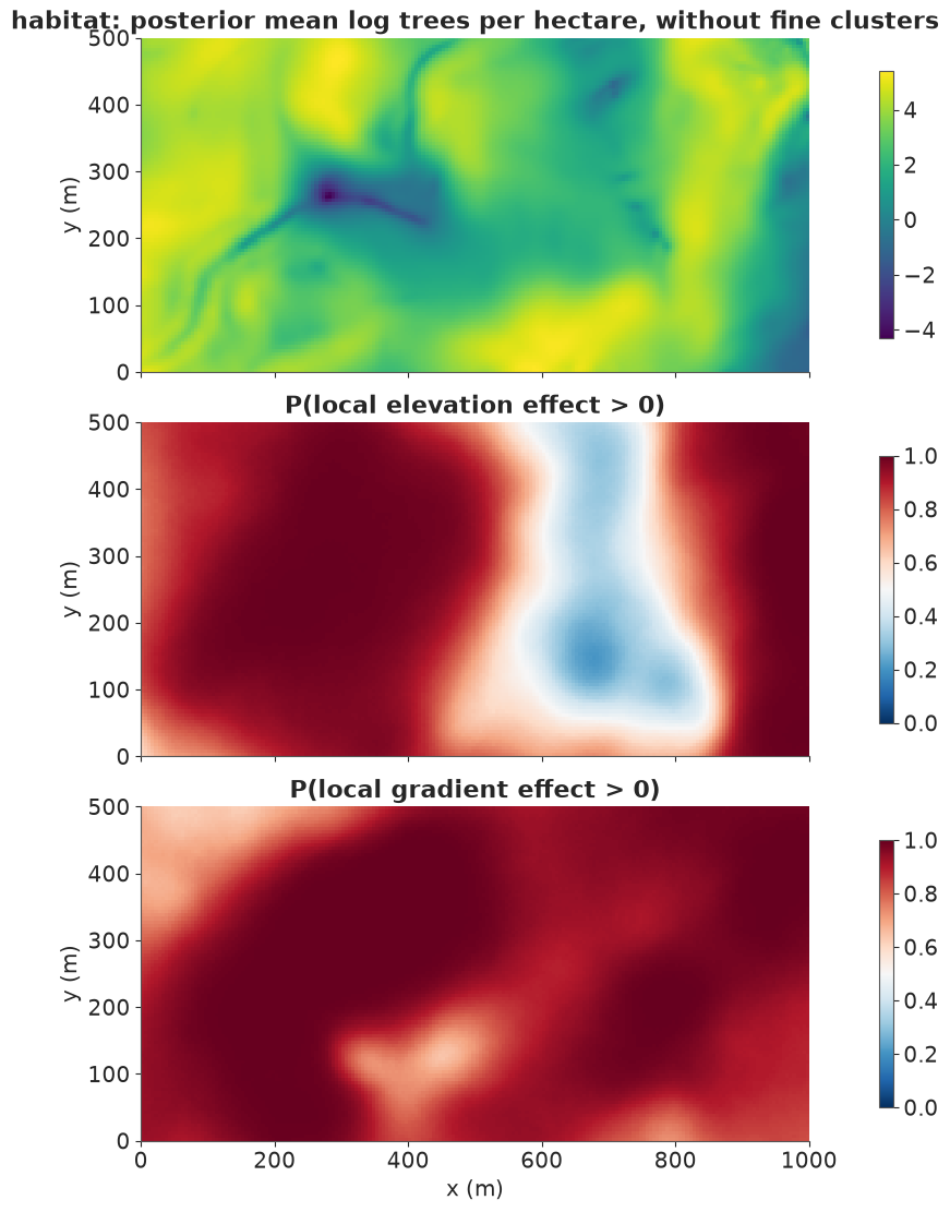
The clustering check. The table has two kinds of replicate. "Fitted clumps" keeps the fitted fine field, which has one coefficient for nearly every cell, so its match to the data is close to guaranteed: it is only an in-sample consistency check. "New clumps" keeps the hyperparameters and draws a fresh fine field, which is the fair test. The observed ratio sits inside that interval from 10 to 100 m, and right at its upper end at 5 m (at or just past the upper end at 5 and 10 m in other runs). So the model captures the clustering at most scales, and its clumps may be slightly too weak at the finest. The expected total matches the 3,604 observed, as a log link with a free intercept should give.
Does the terrain link hold everywhere? No. Averaged over the plot, the species prefers higher,
steeper ground (b_elev about 0.6 and b_grad about 0.5, per sd of elevation and of log
gradient). But the middle map shows the elevation effect changing across the plot. It is
confidently positive over much of the west (roughly x = 100-450) and in the far east, weaker along
the western edge, and on the central plateau, around x = 700 m, it is not clearly different from
zero and may reverse. The printed contrast tests this directly: the effect at (200, 250) exceeds the
effect at (680, 150) by about 2.1 (90% interval 0.6 to 4.0), with probability 0.99. The LogNormal
prior excludes exactly zero variation, but a contrast this size comes from the data. The elevation
link is local. The gradient link is more general: probably positive nearly everywhere, but
confidently so over only about half the plot, and weakest around (450, 130) and in the north-west.
These are associations in one census, not causes. Elevation here is also a proxy for drainage and
soil, and an ell_slope of about 165 m means that features much smaller than that cannot be
resolved.
The fine clumps are strong. s_fine is about 1.1 (a realised sd near 0.95) with a lengthscale
near 7 m, the footprint of a clump of siblings, which is why the habitat map above leaves them out.
Now the survey.
print(f"share of the plot: P(elevation effect > 0) > 0.95: {(p_elev > 0.95).mean():.0%}, < 0.05: {(p_elev < 0.05).mean():.0%}")
print(f"share of the plot: P(gradient effect > 0) > 0.95: {(p_grad > 0.95).mean():.0%}, < 0.05: {(p_grad < 0.05).mean():.0%}")
N_PICK = 5
ranks = (-habitat_ha).argsort(1).argsort(1)
p_top = (ranks < N_PICK).mean(0)
counts_ha = hectares(y[None])[0].ravel()
best = np.argsort(-p_top)[:N_PICK]
raw_best = np.argsort(-counts_ha)[:N_PICK]
table = pd.DataFrame({"hectare": best, "x m": (best % nx_ha) * 100 + 50, "y m": (best // nx_ha) * 100 + 50,
                      "P(top 5)": p_top[best], "habitat index": habitat_ha[:, best].mean(0), "trees counted": counts_ha[best]})
print(table.round(2).to_string(index=False))
print("top five by raw count:", sorted(raw_best.tolist()), "- in common with the model's five:", len(set(best) & set(raw_best)))
for h in sorted(set(raw_best) - set(best)):
    print(f"hectare {h}, raw top five only: {counts_ha[h]:.0f} trees counted, habitat index {habitat_ha[:, h].mean():.0f}, P(top 5) {p_top[h]:.2f}")

fig, ax = plt.subplots(figsize=(9, 3.5), layout="constrained")
im = ax.imshow(p_top.reshape(ny_ha, nx_ha), origin="lower", extent=extent, cmap="magma", vmin=0, vmax=1)
fig.colorbar(im, ax=ax, label=f"P(hectare in the top {N_PICK})", shrink=0.8)
ax.scatter((raw_best % nx_ha) * 100 + 50, (raw_best // nx_ha) * 100 + 50, marker="x", c="w", label="top by raw count")
ax.set(xlabel="x (m)", ylabel="y (m)")
ax.legend(loc="center", labelcolor="w", frameon=False);
share of the plot: P(elevation effect > 0) > 0.95: 39%, < 0.05: 0%
share of the plot: P(gradient effect > 0) > 0.95: 52%, < 0.05: 0%
 hectare  x m  y m  P(top 5)  habitat index  trees counted
       6  650   50      0.99     151.570007          226.0
      20   50  250      0.93     129.619995          210.0
      42  250  450      0.91     126.150002          247.0
       5  550   50      0.73     113.150002          181.0
      48  850  450      0.36      94.059998          134.0
top five by raw count: [5, 6, 20, 28, 42] - in common with the model's five: 4
hectare 28, raw top five only: 155 trees counted, habitat index 82, P(top 5) 0.13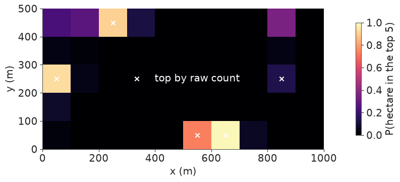
The elevation effect is confidently positive (posterior probability above 0.95) over about 39% of the plot, and the gradient effect over about 52%. Neither is confidently negative anywhere.
For the survey we rank hectares by a habitat index: the expected number of trees with the fine field set to zero, so that a hectare scores for its conditions and not for one lucky family of trees. The index sits below the count of every hectare in the table, by a factor of about 1.5-2. That is expected, since the clumps are where the counted trees stand, and it does not mean the model discounts half the trees.
The recommendation is hectares 6, 20, 42 and 5, with probabilities of being in the top five of about 0.99, 0.93, 0.91 and 0.7, plus hectare 48 as the fifth, with much less confidence (about 0.35).
Four of the five match the raw top counts. The disagreement is the interesting part. Hectare 28, near (850, 250), makes the raw top five but has a low model probability, 0.13 (the white cross on a dark cell), and hectare 48 replaces it despite a lower count. Clumping is part of the reason: 42% of hectare 28's trees stand in three of its 25 squares of 20 m, against 31% in hectare 48. It is not the whole reason, because hectare 42 is more clumped still (45%) and keeps its place. What decides is the habitat estimate, which uses the terrain and the surroundings as well as the count: an index of about 82 for hectare 28, on 155 counted, against 94 for hectare 48, on 134 counted. The fifth place is genuinely uncertain, and hectares along the northern edge compete for it, so a survey that can afford it should add a sixth.
10 · Which steps does a GPU speed up?
To close, we time each stage of the ChEES workflow, from warmup to moving draws off the card.
t0 = time.perf_counter()
_ = summarise(kept_chees)
diagnostics_s = time.perf_counter() - t0
t0 = time.perf_counter()
_ = np.asarray(pos_chees[0])
transfer_s = (time.perf_counter() - t0) * SNAPS  # one snapshot, scaled up to all of them
stages = pd.Series({"warmup (ChEES)": stats_chees["warmup s"], "sampling (ChEES)": stats_chees["sampling s"],
                    "posterior fields": postprocess_s, "diagnostics, on the host": diagnostics_s,
                    "draws, GPU to host": transfer_s}, name="seconds")
print(stages.round(2).to_string())
warmup (ChEES)              112.96
sampling (ChEES)             24.63
posterior fields              1.48
diagnostics, on the host      0.15
draws, GPU to host            0.10
Almost all the time is warmup and sampling: about 113 s and 25 s. Everything else, diagnostics included, takes a second or two at most. Putting together the numbers from every part:
| step | GPU helps? | why, with this notebook's numbers |
|---|---|---|
| Gradients, many chains, large arrays | Yes, by a lot | more than 50x at 128 chains and 24,810 parameters |
| Gradients, one chain, small model | No | 0.5-0.8x at 1,578 parameters |
| ChEES leapfrog steps | Yes | 0.86 ms per gradient, the same as a bare gradient: no overhead |
| NUTS tree building | Partly | about 3.6 ms per gradient: bookkeeping, even with equal trees |
| Warmup | Yes, but it is the main cost | over 80% of the ChEES run: a good start saves more than a faster GPU |
| Posterior fields, predictions | Yes | 3,840 draws of four 20,000-cell fields in about 1.5 s |
| Diagnostics (r_hat, ESS) | Not needed | a fraction of a second, on the CPU |
| Moving draws to the host | Not a bottleneck | a fraction of a second; keep only what you need, as memory adds up |
| Compilation | Worse | 2 s against 0.4 s, and each new shape recompiles |
| Python, I/O, data preparation | No | not array arithmetic |
Use a GPU for ensemble sampling when the gradient is dominated by large array operations, the
posterior is roughly unimodal, and you can use float32 or have a data-centre card. Stay with
nutpie on a CPU when the model is small, is full of scan and control flow, or has modes that a
shared tuning would hide, or when one reliable run in a few minutes already answers the question.
Summary
- The terrain link is local. The elevation effect is confidently positive over about 39% of the plot and confidently negative nowhere; between the western rise and the central plateau it differs by about 2.1 (90% interval 0.6 to 4.0). The gradient effect is more general, confidently positive over about half the plot. These are associations in one census, and the fields cannot resolve features much smaller than about 165 m.
- Clumps and habitat can be told apart. The fine field has a lengthscale near 7 m and a realised sd near 0.95. With fresh clumps, the model reproduces the variance-to-mean ratio from 10 to 100 m, and its clumps may be slightly too weak at 5 m.
- The survey should use hectares 6, 20, 42 and 5, each with a probability of 0.7 or more of being in the top five, plus hectare 48 (about 0.35). Hectare 28 has more trees than hectare 48 but a lower habitat index; the fifth place is uncertain, so a sixth hectare is worth adding.
- A GPU speeds up large batches of large arrays. A batched gradient is more than 50x faster at 128 chains and 24,810 parameters, but slower than the CPU for one chain on a small model. On a consumer card float32 is about 17x faster than float64, and its log-density error here (sd about 0.04) is negligible for ChEES.
- NUTS on a GPU pays for bookkeeping, not for uneven trees: almost every tree here had 127 steps, yet each NUTS gradient cost about 3.6 ms against 0.86 ms for ChEES.
- ChEES-HMC needs a metric and a check for stragglers. Without the diagonal metric, ESS is several times lower and r_hat too high; one stuck chain can inflate the trajectory for all of them, and restarting it from a healthy copy during warmup fixes that. The result is about 65x nutpie's worst-case ESS per second (55-70x across runs), with warmup taking over 80% of the time.
- MEADS fails quietly from a cold start (step size zero, r_hat in the hundreds, acceptance near 0.8) and is excellent from the ChEES ensemble, at about 40x nutpie. It needed a smaller step-size multiplier, 16 chains per fold, and LogNormal rather than half-normal priors on field sds.
- The speed-up is hardware and algorithm together: an estimated 25-30x from the GPU and 2-2.5x from ChEES, each useless without the other. On 8 CPU cores nutpie wins. A poorly configured baseline would have inflated the headline to about 200x.
- An ensemble is only as healthy as its worst chain. Acceptance looked fine in both failures run here, and the stragglers appeared on some seeds but not others. Trust r_hat from dispersed starts, per-chain plots and checks over several seeds.
Try it yourself
- Scale it up. With a GPU, set
CHAINSto 512 or 1024. (The CPU-estimate rows then drop out, as the CPU is not timed above 128 chains.) Does worst-case ESS per second keep rising, or does warmup, which does not get shorter, take over? - Pay for precision. Run ChEES in float64 inside
precision("float64"). How close does the time come to the 17x penalty, and does the posterior change? - Break it, then diagnose it. Remove the culling step and run four or five seeds, printing
Land the divergences each time. Then go back topm.HalfNormalfor the field sds and see what MEADS does.