The setting
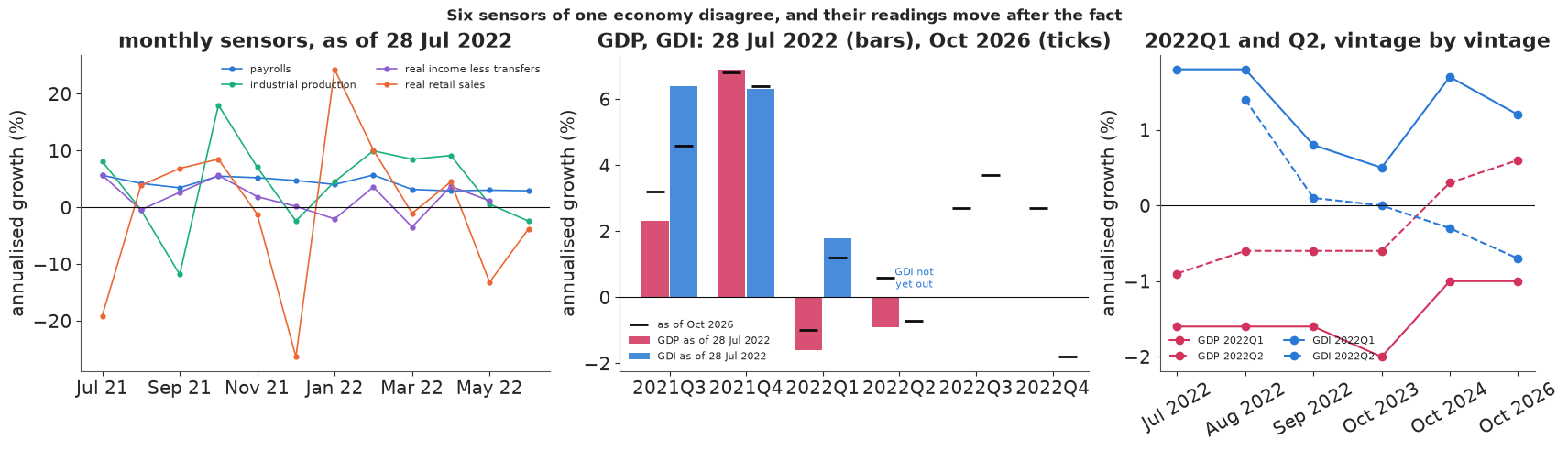
On 28 July 2022 the Bureau of Economic Analysis published its first ("advance") estimate of US output in the second quarter: real GDP had fallen at an annual rate of 0.9%, after falling 1.6% in the first quarter. Two quarters of falling GDP is the newspaper definition of a recession, and for a few weeks the question "is the US in a recession?" was everywhere. Other numbers disagreed. Employers had added about 2.7 million jobs in the first half of the year, industrial production was rising, and a month later the income-side measure of output, gross domestic income (GDI), said the economy had grown in both quarters. The NBER's Business Cycle Dating Committee, which dates US recessions, does not use the two-quarter rule; it looks at a set of monthly indicators of production, employment, income and sales, and it never declared a recession in 2022.
This is a textbook problem in disguise: several imperfect sensors measure one thing nobody observes. GDP adds up spending, GDI adds up incomes; in principle they are equal, in practice they differ by measurement error, and neither is the truth (Nalewaik 2010). Monthly indicators see the same economy more often, but each only partly tracks output. And every one of them is revised, sometimes for years: by October 2024 the second-quarter fall in GDP had become a rise, while second-quarter GDI had become a fall. Statistically, the right reading of all of this is a posterior for the latent output path given every sensor, with each sensor's noise learned from the data. Aruoba, Diebold, Nalewaik, Schorfheide & Song (2016) did this for GDP and GDI ("GDPplus", now published by the Philadelphia Fed); dynamic factor models that mix monthly and quarterly data go back to Stock & Watson (1989) and Mariano & Murasawa (2003), and became the standard tool for nowcasting (Giannone, Reichlin & Small 2008; Bańbura et al. 2013). Real-time data sets that keep every vintage (Croushore & Stark 2001) let us replay what was knowable on a given day.
We stand on 28 July 2022 and ask: what is the probability that US output actually fell in the first half of 2022? Then we ask it again on five later dates, once with GDP alone and once with all six sensors, and see which answer holds up. E90 covered vintages, nowcasts and the cost of waiting for revisions in detail; here revisions are a fact of life and the lesson is fusion: how sensors of different frequency, timing and quality combine in one likelihood, and what goes wrong when one of them is modelled too kindly.
| part | question | tool |
|---|---|---|
| A | What did each sensor say, and when? | ALFRED vintages, growth rates, revision sizes |
| B | How do six sensors measure one economy? | a monthly latent path, mixed-frequency loadings, correlated GDP-GDI errors; integrating the path out; prior predictive |
| C | What does GDP alone say in July 2022? | the one-sensor model; what it can and cannot learn about its own noise |
| D | What does fusion say, and what goes wrong first? | a naive fused model, a residual check, persistent sensor errors |
| E | How did the answer move as the data were revised? | replaying six vintages with GDP alone and fused |
| F | Which sensor carries the answer? | dropping sensors, fixing the GDP-GDI error correlation |
| G | Does the fused model fit, and was it right? | posterior predictive checks, a held-out GDP print, scoring July 2022 against 2026 |
| H | Should a forecaster have called a recession? | a decision threshold from the costs of the two errors |
import os

for _v in ("OPENBLAS_NUM_THREADS", "OMP_NUM_THREADS", "MKL_NUM_THREADS"):
    os.environ.setdefault(_v, "1")      # one BLAS thread per chain: four chains run in parallel

import logging
import sys
import time
import warnings

import arviz as az
import matplotlib.pyplot as plt
import numpy as np
import nutpie
import pandas as pd
import pymc as pm
import pytensor.tensor as pt
from scipy import stats

from pymc_challenges import data

# ArviZ registers a lazy placeholder module for jax that matplotlib would then try to import; remove it,
# but only if it is that placeholder (a real, imported jax has a __file__ and is left alone).
if "jax" in sys.modules and getattr(sys.modules["jax"], "__file__", None) is None:
    del sys.modules["jax"]
RANDOM_SEED = 98
rng = np.random.default_rng(RANDOM_SEED)
az.style.use("arviz-variat")
logging.getLogger("pymc").setLevel(logging.WARNING)
warnings.filterwarnings("ignore", category=RuntimeWarning, module="arviz")
warnings.filterwarnings("ignore", message=".*sample_stats.*")
warnings.filterwarnings("ignore", message=".*Potential.*")
pd.set_option("display.width", 170)
pd.set_option("display.max_columns", 20)
T_START = time.time()

BLUE, ORANGE, AQUA, PURPLE, RED = "#2a78d6", "#eb6834", "#1baf7a", "#8e5bd0", "#d2335c"
INK, MUTED, LIGHT = "#0b0b0b", "#8a8984", "#d9d8d3"
A. Six sensors, six vintages
ALFRED keeps every version of a FRED series: asking for a series "as of" a date returns exactly what a user downloading it that day would have seen. The cached file holds six of those snapshots for each sensor, plus the first published value of GDP and GDI growth for every quarter 2014Q3-2019Q4.
data.describe("e98_alfred_vintages")
raw = data.load("e98_alfred_vintages")
raw["date"] = pd.to_datetime(raw["date"])
VINTAGES = ["2022-07-28", "2022-08-25", "2022-09-29", "2023-10-01", "2024-10-01", "2026-10-01"]
VLABEL = {"2022-07-28": "Jul 2022", "2022-08-25": "Aug 2022", "2022-09-29": "Sep 2022",
          "2023-10-01": "Oct 2023", "2024-10-01": "Oct 2024", "2026-10-01": "Oct 2026"}
MSER = ["payrolls", "indpro", "income_ex_transfers", "retail_sales"]
MNAME = {"payrolls": "payrolls", "indpro": "industrial production",
         "income_ex_transfers": "real income less transfers", "retail_sales": "real retail sales"}
print(raw.groupby("series").size().to_string())
print("\nlast observation in each vintage:")
last = raw[raw.vintage.isin(VINTAGES)].groupby(["vintage", "series"]).date.max().unstack()
print(last.apply(lambda c: c.dt.strftime("%Y-%m")).to_string())
e98_alfred_vintages: US output indicators as they stood on given dates. Long format: series (gdp, gdi = annualised quarterly % growth of real GDP / real GDI, dated by the first day of the quarter; payrolls (thousands), indpro (index), income_ex_transfers (billions of chained dollars, SAAR), retail_sales (millions of 1982-84 dollars, deflated by the CPI), all seasonally adjusted monthly levels, dated by the first day of the month), vintage (the date at which the value stood; ALFRED serves the latest release on or before it), date, value. Six vintages hold complete histories 2011-10 to 2022-12 (2022-07-28, 2022-08-25, 2022-09-29, 2023-10-01, 2024-10-01, 2026-10-01; later observations dropped); the other rows are the FIRST published value of each quarter 2014Q3-2019Q4 of gdp and gdi, at the first monthly vintage (requested on the 15th) containing it.
  source: ALFRED (ArchivaL Federal Reserve Economic Data), Federal Reserve Bank of St. Louis (alfred.stlouisfed.org); the series are US government statistics in the public domain, compiled by BEA (real GDP growth A191RL1Q225SBEA, real GDI growth A261RL1Q225SBEA, real personal income excluding current transfer receipts W875RX1), BLS (total nonfarm payrolls PAYEMS), the Federal Reserve Board (industrial production INDPRO) and the Census Bureau (advance retail and food services sales RSAFS, which FRED deflates by the CPI, CPIAUCSL, to give real retail sales RRSFS). The URL is one of about 190 vintage requests (6 series x 6 dates, plus 75 monthly vintages of the two growth-rate series); SNAPSHOT assembled by tools/build_e98_data.py - keep the cached file in data/.
  url:    https://alfred.stlouisfed.org/graph/alfredgraph.csv?id=A191RL1Q225SBEA&vintage_date=2022-07-28
series
gdi                    285
gdp                    286
income_ex_transfers    792
indpro                 795
payrolls               795
retail_sales           795

last observation in each vintage:
series          gdi      gdp income_ex_transfers   indpro payrolls retail_sales
vintage
2022-07-28  2022-01  2022-04             2022-05  2022-06  2022-06      2022-06
2022-08-25  2022-04  2022-04             2022-06  2022-07  2022-07      2022-07
2022-09-29  2022-04  2022-04             2022-07  2022-08  2022-08      2022-08
2023-10-01  2022-10  2022-10             2022-12  2022-12  2022-12      2022-12
2024-10-01  2022-10  2022-10             2022-12  2022-12  2022-12      2022-12
2026-10-01  2022-10  2022-10             2022-12  2022-12  2022-12      2022-12
The snapshots end at different months for different sensors. On 28 July 2022 GDP already had a second-quarter number but GDI did not: BEA publishes GDI a month after GDP, with the second estimate. Payrolls, industrial production and retail sales were known through June, real income only through May. This uneven frontier is the ragged edge of real-time data. (The later vintages were cut at December 2022: our question is about the first half of 2022, and a window that ends in the same month for every vintage keeps the comparisons clean.)
All sensors go on one scale: annualised percentage growth. GDP and GDI arrive in that form. For a monthly level $L_t$ we use $x_t = 1200\,(\log L_t - \log L_{t-1})$, the monthly log change at an annual rate. The window is January 2012 to December 2022. The pandemic months March 2020 to June 2021 (and the quarters 2020Q1-2021Q2) are masked in every sensor: output fell by a third at an annual rate in 2020Q2 and rebounded as fast, and a model of ordinary fluctuations has nothing to learn from that. Masking is not deleting the months: the latent path still runs through them, just without readings.
MONTHS = pd.date_range("2012-01-01", "2022-12-01", freq="MS")
QUARTERS = pd.date_range("2012-04-01", "2022-10-01", freq="QS")   # quarters whose 5 weighted months are inside
T, NQ = len(MONTHS), len(QUARTERS)
COVID_M = (MONTHS >= "2020-03-01") & (MONTHS <= "2021-06-01")
COVID_Q = (QUARTERS >= "2020-01-01") & (QUARTERS <= "2021-04-01")
Q1, Q2 = QUARTERS.get_loc("2022-01-01"), QUARTERS.get_loc("2022-04-01")


def snapshot(vintage):
    """Monthly growth (T) per monthly sensor and quarterly growth (NQ) for GDP and GDI, as of a vintage."""
    d = raw[raw.vintage == vintage]
    monthly = {}
    for s in MSER:
        lev = d[d.series == s].set_index("date")["value"].sort_index()
        x = (1200 * np.log(lev).diff()).reindex(MONTHS).to_numpy().copy()
        x[COVID_M] = np.nan
        monthly[s] = x
    quarterly = {}
    for s in ("gdp", "gdi"):
        y = d[d.series == s].set_index("date")["value"].reindex(QUARTERS).to_numpy().copy()
        y[COVID_Q] = np.nan
        quarterly[s] = y
    return monthly, quarterly


SNAP = {v: snapshot(v) for v in VINTAGES}
rows = []
for v in VINTAGES:
    m, q = SNAP[v]
    h1 = slice(MONTHS.get_loc("2022-01-01"), MONTHS.get_loc("2022-06-01") + 1)
    row = {"vintage": VLABEL[v], "GDP Q1": q["gdp"][Q1], "GDP Q2": q["gdp"][Q2],
           "GDI Q1": q["gdi"][Q1], "GDI Q2": q["gdi"][Q2]}
    row.update({f"{s} H1": np.nanmean(m[s][h1]) for s in MSER})
    rows.append(row)
tab_a = pd.DataFrame(rows).set_index("vintage")
print("annualised growth (%) in the first half of 2022, as published at each vintage "
      "(monthly sensors: mean over the months then available)")
print(tab_a.round(1).to_string())
pre = (MONTHS >= "2012-01-01") & (MONTHS < "2020-01-01")
m26, q26 = SNAP["2026-10-01"]
print("\n2012-2019 (Oct 2026 vintage): mean and sd of each sensor's growth")
print(pd.DataFrame({s: [np.nanmean(m26[s][pre]), np.nanstd(m26[s][pre])] for s in MSER}
                   | {s: [np.nanmean(q26[s][QUARTERS < "2020-01-01"]), np.nanstd(q26[s][QUARTERS < "2020-01-01"])]
                      for s in ("gdp", "gdi")}, index=["mean", "sd"]).round(2).to_string())
annualised growth (%) in the first half of 2022, as published at each vintage (monthly sensors: mean over the months then available)
          GDP Q1  GDP Q2  GDI Q1  GDI Q2  payrolls H1  indpro H1  income_ex_transfers H1  retail_sales H1
vintage
Jul 2022    -1.6    -0.9     1.8     NaN          3.6        5.1                     0.6              3.5
Aug 2022    -1.6    -0.6     1.8     1.4          3.7        4.8                     0.1              4.1
Sep 2022    -1.6    -0.6     0.8     0.1          3.5        4.7                     0.0              4.5
Oct 2023    -2.0    -0.6     0.5     0.0          3.5        3.5                    -3.4              4.0
Oct 2024    -1.0     0.3     1.7    -0.3          3.4        3.2                    -3.1              3.4
Oct 2026    -1.0     0.6     1.2    -0.7          3.4        0.9                    -3.5              4.6

2012-2019 (Oct 2026 vintage): mean and sd of each sensor's growth
      payrolls  indpro  income_ex_transfers  retail_sales   gdp   gdi
mean      1.66    0.67                 2.67          2.07  2.49  2.24
sd        0.68    5.55                 9.26          6.86  1.47  1.91
The table is the whole controversy in numbers. In July 2022 GDP said -1.6 and -0.9, while every monthly sensor said growth: payrolls at 3.6% a year over the first half (their 2012-2019 average is 1.7%), industrial production at 5.1%, retail sales at 3.5%, real income at 0.6%. When GDI arrived in August it said +1.8 and +1.4, and the September annual update cut it to +0.8 and +0.1. By October 2024 GDP's second quarter had turned positive and GDI's negative: the two measures of output swapped sign.
The monthly sensors were revised as well, and two of them a lot. Industrial production's first-half growth fell from 5.1% in the July 2022 vintage to 0.9% in the October 2026 one; real income less transfers went from +0.6% to -3.5%. Payrolls (3.6 to 3.4) and retail sales (3.5 to 4.6) changed less. Keep this in mind: the model below will treat a monthly reading as final once published.
The second table shows why reading any single month is hopeless: real income growth has a standard deviation of about 9 points from month to month around a mean of 2.7, retail sales about 7 and industrial production about 5.5. Payrolls are smooth (sd 0.7); GDP and GDI quarterly growth have sds of about 1.5 and 1.9.
fig, axes = plt.subplots(1, 3, figsize=(17, 4.8), width_ratios=[1.25, 1.25, 1])
m0, q0 = SNAP["2022-07-28"]
win = (MONTHS >= "2021-07-01") & (MONTHS <= "2022-06-01")
ax = axes[0]
for s, c in zip(MSER, (BLUE, AQUA, PURPLE, ORANGE)):
    ax.plot(np.arange(win.sum()), m0[s][win], "o-", color=c, lw=1.2, ms=3.5, label=MNAME[s])
ax.axhline(0, color=INK, lw=0.8)
ax.set_xticks(np.arange(0, win.sum(), 2), [d.strftime("%b %y") for d in MONTHS[win][::2]])
ax.set(title="monthly sensors, as of 28 Jul 2022", ylabel="annualised growth (%)")
ax.legend(fontsize=8, ncols=2)
ax = axes[1]
qwin = QUARTERS >= "2021-07-01"
xq = np.arange(qwin.sum())
for j, (s, c) in enumerate((("gdp", RED), ("gdi", BLUE))):
    ax.bar(xq + (j - 0.5) * 0.38, q0[s][qwin], width=0.36, color=c, alpha=0.85,
           label=f"{s.upper()} as of 28 Jul 2022")
    ax.plot(xq + (j - 0.5) * 0.38, q26[s][qwin], "_", color=INK, ms=14, mew=2,
            label="as of Oct 2026" if j == 0 else None)
ax.axhline(0, color=INK, lw=0.8)
ax.set_xticks(xq, [f"{d.year}Q{(d.month - 1) // 3 + 1}" for d in QUARTERS[qwin]])
ax.set(title="GDP, GDI: 28 Jul 2022 (bars), Oct 2026 (ticks)", ylabel="annualised growth (%)")
ax.text(xq[Q2 - np.flatnonzero(qwin)[0]] + 0.19, 0.3, "GDI not\nyet out", ha="center", fontsize=8, color=BLUE)
ax.legend(fontsize=8)
ax = axes[2]
for s, c in (("GDP", RED), ("GDI", BLUE)):
    for qq, ls in (("Q1", "-"), ("Q2", "--")):
        ax.plot(np.arange(len(VINTAGES)), tab_a[f"{s} {qq}"].to_numpy(), ls, marker="o", color=c,
                label=f"{s} 2022{qq}")
ax.axhline(0, color=INK, lw=0.8)
ax.set_xticks(np.arange(len(VINTAGES)), [VLABEL[v] for v in VINTAGES], rotation=30)
ax.set(title="2022Q1 and Q2, vintage by vintage", ylabel="annualised growth (%)")
ax.legend(fontsize=8, ncols=2)
fig.suptitle("Six sensors of one economy disagree, and their readings move after the fact", fontsize=12);
How noisy is a fresh GDP print?
A number that has just been published will be revised; one that has been through several annual updates mostly will not. For the 22 quarters 2014Q3-2019Q4 we have the first published growth rate and the value in the October 2026 vintage. Their difference measures the revision noise of a fresh print, and we will add that much extra variance to every fresh GDP or GDI reading. The rule for "fresh" is deliberately simple: a quarter is fresh at a vintage if the vintage falls less than 245 days after the quarter's first day, that is, within about five months of the quarter's end. For 2022Q1 that switch happens between the August and September 2022 vintages, which roughly coincides with the annual update of 29 September 2022. It is cruder elsewhere: in the July and August 2022 vintages it counts 2021Q3 and 2021Q4 as mature, though neither had yet been through an annual update, and it treats a quarter as fully mature after one update, though 2022Q1 went on to move from -1.6 to -2.0 and then to -1.0 in later revisions.
Three more simplifications. The revision size is measured with hindsight, against the October 2026 vintage, which a forecaster in July 2022 could not have done (calibrating against the latest vintage before each replay date would remove that look-ahead). GDP's revisions also have a mean: on average they went up, by about half a point. We fold that into the variance by using the root mean square rather than modelling it as a bias, which would have pushed fresh negative prints up further. And we treat the revision variance as known, though 22 quarters pin a standard deviation down only to about ±15%.
first = raw[~raw.vintage.isin(VINTAGES)]
TAU = {}
for s in ("gdp", "gdi"):
    f = first[first.series == s].set_index("date")["value"]
    latest = raw[(raw.series == s) & (raw.vintage == "2026-10-01")].set_index("date")["value"].reindex(f.index)
    rev = latest - f
    TAU[s] = float(np.sqrt(np.mean(rev**2)))
    print(f"{s.upper()}: {len(rev)} quarters, revision first -> Oct 2026: mean {rev.mean():+.2f}, "
          f"sd {rev.std():.2f}, root mean square {TAU[s]:.2f} percentage points; "
          f"largest {rev.abs().max():.1f}")


def fresh_flags(vintage):
    return ((pd.Timestamp(vintage) - QUARTERS).days < 245).astype(float)
GDP: 22 quarters, revision first -> Oct 2026: mean +0.46, sd 1.38, root mean square 1.42 percentage points; largest 3.4
GDI: 22 quarters, revision first -> Oct 2026: mean +0.20, sd 1.49, root mean square 1.46 percentage points; largest 3.4
A fresh GDP growth rate moves by about 1.4 points on its way to the current vintage, GDI by about 1.5. That is as large as a typical quarter's growth, and on its own it says that -1.6 and -0.9 were weak evidence of falling output. How weak depends on everything else we know - which is what the model is for.
B. One economy, many sensors
The latent path
Let $g_t$ be the annualised growth of US output in month $t$, $t = 1, \dots, 132$ (January 2012 to December 2022). Nobody observes it. We give it the simplest dynamics that can work, a stationary AR(1) around a mean:
$$g_t - \mu = \phi\,(g_{t-1} - \mu) + s\,\varepsilon_t, \qquad \varepsilon_t \sim \mathcal N(0, 1),$$
with $\mu \sim \mathcal N(2, 1)$ (long-run US growth has been around 2% a year), $\phi \sim \mathrm{Beta}(2, 2)$ and $s \sim \mathrm{LogNormal}(\log 2.5, 0.5)$.
Quarterly sensors: GDP and GDI
A quarterly growth rate compares the average level of output in two quarters. Writing quarter levels as averages of three monthly log levels and expanding the difference gives the triangle weights of Mariano & Murasawa (2003): the annualised growth of quarter $q$ whose last month is $t$ is
$$\gamma_q = \tfrac19\left(g_t + 2g_{t-1} + 3g_{t-2} + 2g_{t-3} + g_{t-4}\right),$$
a weighted average of five monthly growth rates, two of them from the previous quarter. Collect the weights in a $43 \times 132$ matrix $A$, so $\gamma = Ag$. GDP and GDI both measure $\gamma$:
$$\begin{pmatrix} y^{\rm GDP}_q \\ y^{\rm GDI}_q \end{pmatrix} \sim \mathcal N\!\left( \begin{pmatrix} \gamma_q \\ \gamma_q \end{pmatrix}, \begin{pmatrix} \sigma_P^2 + \tau_P^2 f_q & \rho\,\sigma_P\sigma_I \\ \rho\,\sigma_P\sigma_I & \sigma_I^2 + \tau_I^2 f_q\end{pmatrix}\right),$$
where $f_q = 1$ for a fresh print. Both load on $\gamma_q$ with coefficient one: that fixes the scale of $g$. Their mature errors may be correlated, $\rho$ (they share source data, and Aruoba et al. (2016) found the correlation matters and is hard to pin down). Priors: $\sigma_P, \sigma_I \sim \mathrm{LogNormal}(0, 0.5)$ (median 1 point), $(\rho + 1)/2 \sim \mathrm{Beta}(2, 2)$.
Monthly sensors
Each monthly indicator $k$ is an affine, noisy reading of the same month's output growth,
$$x_{k,t} = a_k + \lambda_k g_t + u_{k,t}, \qquad u_{k,t} = \psi_k u_{k,t-1} + \sigma_k \eta_{k,t},$$
with its own intercept $a_k$ (payrolls grow slower than output because productivity grows), loading $\lambda_k > 0$ and an error that may persist from month to month ($\psi_k$). The first naive model will set $\psi_k = 0$. Priors: $a_k \sim \mathcal N(0, 3)$, $\lambda_k \sim \mathrm{LogNormal}(0, 0.75)$, $\sigma_k \sim \mathrm{LogNormal}(\log 3, 1)$, $\psi_k \sim \mathrm U(-0.99, 0.99)$.
The ragged edge costs nothing
A reading that does not exist - GDI for 2022Q2 on 28 July, real income for June, a masked pandemic month - is simply left out of the likelihood. There is nothing to impute: the latent path is defined for every month, and each sensor contributes where it has reported. "GDP alone" is the same model with every other sensor switched off, and "as of 28 July 2022" is the same model with the readings published after that date switched off.
Integrating the path out
Sampling 132 latent months jointly with the sensor parameters works, but the posterior has ridges (a smoother economy versus more persistent sensor errors) that cost NUTS thousands of gradient evaluations per draw. In prototype runs not shown in this notebook, sampling the path directly (centred or non-centred) gave r-hat of 1.05-1.14 and bulk ESS of 20-90 on the fused model, or hundreds of divergences; Try it yourself 1 asks for a model where you meet this for yourself. Given the parameters $\theta$, though, everything is linear and Gaussian, so the path can be integrated out exactly - the same thing a Kalman filter does (E13), done in one solve.
Write every reading, after a transformation with unit Jacobian, as $y_i = c_i + h_i^\top g + e_i$ with independent $e_i \sim \mathcal N(0, v_i)$: a monthly reading with AR(1) error becomes the quasi-difference $x_{k,t} - \psi_k x_{k,t-1} = a_k(1 - \psi_k) + \lambda_k(g_t - \psi_k g_{t-1}) + \sigma_k\eta_{k,t}$ (the first reading after a gap keeps its stationary variance), and GDI becomes its conditional distribution given GDP. With the AR(1) prior precision $Q_0$ (tridiagonal), the posterior precision of the path and the marginal likelihood are
$$Q = Q_0 + \sum_i \frac{h_i h_i^\top}{v_i}, \qquad b = \sum_i \frac{h_i r_i}{v_i}, \qquad \log p(y \mid \theta) = -\tfrac12\Bigl[n\log 2\pi + \sum_i \log v_i - \log|Q_0| + \log|Q| + \sum_i \frac{r_i^2}{v_i} - b^\top Q^{-1} b\Bigr],$$
with $r_i = y_i - c_i - \mu\,h_i^\top \mathbf 1$ (matrix determinant lemma plus Woodbury). Each monthly sensor adds a tridiagonal band to $Q$ and the quarterly sensors a band five months wide, so $Q$ is a narrow-band $132 \times 132$ matrix; one Cholesky factor gives everything. This is the "precision-based" state-space method of Rue & Held (2005) and Chan & Jeliazkov (2009). After sampling $\theta$, we draw the path from $g \mid y, \theta \sim \mathcal N(\mu\mathbf 1 + Q^{-1}b,\; Q^{-1})$, one exact draw per posterior draw.
The function below is written once for NumPy and PyTensor (the xp argument): the model uses it for the
likelihood, NumPy for the path draws and the checks.
A = np.zeros((NQ, T))
for j, qs in enumerate(QUARTERS):
    t_last = MONTHS.get_loc(qs) + 2
    A[j, t_last - np.arange(5)] = np.array([1, 2, 3, 2, 1]) / 9
EYE, SUP = np.eye(T), np.eye(T, k=1)
ALL = ("gdp", "gdi") + tuple(MSER)


def ar1_precision(phi, s):
    """Precision of a stationary AR(1) path with innovation sd s (tridiagonal)."""
    inner = np.r_[0.0, np.ones(T - 2), 0.0]
    return (EYE + phi**2 * np.diag(inner) - phi * (SUP + SUP.T)) / s**2


def sensor_algebra(p, d, xp):
    """Q_data, b, sum r^2/v, sum log v, n for parameters p and readings d (NumPy or PyTensor)."""
    mu, sp, si = p["mu"], p["sig_gdp"], p["sig_gdi"]
    vp = sp**2 + TAU["gdp"] ** 2 * d["fresh"]
    vi = si**2 + TAU["gdi"] ** 2 * d["fresh"]
    cov = p["rho"] * sp * si
    kap = cov / vp                                   # GDI given GDP: regression coefficient
    vic = vi - cov**2 / vp                           # ... and conditional variance
    rp = d["gdp_y"] - mu
    ri = d["gdi_y"] - kap * d["gdp_y"] - (1 - kap) * mu
    wq = d["gdp_ok"] / vp + d["gdi_ok"] * (1 - kap) ** 2 / vic
    Q = A.T @ (wq[:, None] * A)
    b = A.T @ (d["gdp_ok"] * rp / vp + d["gdi_ok"] * (1 - kap) * ri / vic)
    quad = xp.sum(d["gdp_ok"] * rp**2 / vp + d["gdi_ok"] * ri**2 / vic)
    logv = xp.sum(d["gdp_ok"] * xp.log(vp) + d["gdi_ok"] * xp.log(vic))
    n = xp.sum(d["gdp_ok"]) + xp.sum(d["gdi_ok"])
    diag, off = 0 * mu + np.zeros(T), 0 * mu + np.zeros(T - 1)
    for k in MSER:
        ic, i0, x, xl = d[f"ic_{k}"], d[f"i0_{k}"], d[f"x_{k}"], d[f"xl_{k}"]
        a, lam, sig = p[f"a_{k}"], p[f"lam_{k}"], p[f"sig_{k}"]
        psi = d["use_ar"] * p[f"psi_{k}"]
        w, w0 = lam**2 / sig**2, lam**2 * (1 - psi**2) / sig**2
        rc = ic * (x - psi * xl - (a + lam * mu) * (1 - psi))      # quasi-differenced readings
        r0 = i0 * (x - a - lam * mu)                               # first reading of a run
        diag = diag + w * ic + w * psi**2 * xp.concatenate([ic[1:], np.zeros(1)]) + w0 * i0
        off = off - w * psi * ic[1:]
        b = b + lam / sig**2 * (rc - psi * xp.concatenate([rc[1:], np.zeros(1)])) + w0 / lam * r0
        quad = quad + (xp.sum(rc**2) + (1 - psi**2) * xp.sum(r0**2)) / sig**2
        logv = logv + xp.sum(ic) * xp.log(sig**2) + xp.sum(i0) * xp.log(sig**2 / (1 - psi**2))
        n = n + xp.sum(ic) + xp.sum(i0)
    off_full = xp.concatenate([off, np.zeros(1)])
    Q = Q + diag[:, None] * EYE + off_full[:, None] * SUP + off_full[None, :] * SUP.T
    return Q, b, quad, logv, n


def readings(vintage, sensors=ALL, use_ar=1.0, rho=None, hide=()):
    """The data arrays for one fit: which readings exist at this vintage, for these sensors."""
    m, q = SNAP[vintage]
    d = {"fresh": fresh_flags(vintage)}
    gdp_ok = ~np.isnan(q["gdp"]) & ("gdp" in sensors)
    for qq in hide:                                  # readings held out on purpose (part G)
        gdp_ok[QUARTERS.get_loc(qq)] = False
    gdi_ok = ~np.isnan(q["gdi"]) & gdp_ok & ("gdi" in sensors)
    d |= {"gdp_y": np.nan_to_num(q["gdp"]), "gdp_ok": gdp_ok.astype(float),
          "gdi_y": np.nan_to_num(q["gdi"]), "gdi_ok": gdi_ok.astype(float)}
    for k in MSER:
        x = m[k]
        ok = ~np.isnan(x) & (k in sensors)
        ic = np.r_[False, ok[:-1]] & ok
        d |= {f"x_{k}": np.nan_to_num(x), f"xl_{k}": np.r_[0.0, np.nan_to_num(x[:-1])],
              f"ic_{k}": ic.astype(float), f"i0_{k}": (ok & ~ic).astype(float)}
    d |= {"use_ar": np.array(use_ar), "rho_free": np.array(float(rho is None)),
          "rho_value": np.array(0.0 if rho is None else float(rho))}
    return d
Before trusting 40 lines of algebra, we check them. For one parameter point (random sensor parameters) we compute the log-likelihood of the 28 July 2022 data two ways: with the banded formula above, and by brute force - stacking every raw reading into one vector and evaluating a multivariate normal with the full covariance $M\Sigma_g M^\top + \Sigma_e$ (AR(1) blocks within each run of a monthly sensor, 2 × 2 GDP-GDI blocks per quarter).
def loglik_banded(p, d):
    Qd, b, quad, logv, n = sensor_algebra(p, d, np)
    L = np.linalg.cholesky(ar1_precision(p["phi"], p["s"]) + Qd)
    w = np.linalg.solve(L, b)
    logdet_q0 = -2 * T * np.log(p["s"]) + np.log(1 - p["phi"] ** 2)
    return -0.5 * (n * np.log(2 * np.pi) + logv - logdet_q0 + 2 * np.log(np.diag(L)).sum() + quad - w @ w)


def loglik_brute(p, d):
    rows, M, mean = [], [], []
    for s in ("gdp", "gdi"):
        for j in np.flatnonzero(d[f"{s}_ok"]):
            rows.append((s, j)); M.append(A[j]); mean.append(p["mu"])
    for k in MSER:
        for t in np.flatnonzero(d[f"ic_{k}"] + d[f"i0_{k}"]):
            rows.append((k, t)); M.append(p[f"lam_{k}"] * EYE[t])
            mean.append(p[f"a_{k}"] + p[f"lam_{k}"] * p["mu"])
    M, mean = np.array(M), np.array(mean)
    y = np.array([d[f"{s}_y"][j] if s in ("gdp", "gdi") else d[f"x_{s}"][j] for s, j in rows])
    S = M @ np.linalg.inv(ar1_precision(p["phi"], p["s"])) @ M.T
    run = {k: np.cumsum(d[f"i0_{k}"]) for k in MSER}               # run id of each month
    for i, (si, ti) in enumerate(rows):
        for j, (sj, tj) in enumerate(rows):
            if si in ("gdp", "gdi") and sj in ("gdp", "gdi") and ti == tj:
                vp = p["sig_gdp"] ** 2 + TAU["gdp"] ** 2 * d["fresh"][ti]
                vi = p["sig_gdi"] ** 2 + TAU["gdi"] ** 2 * d["fresh"][ti]
                S[i, j] += vp if si == sj == "gdp" else vi if si == sj == "gdi" else p["rho"] * p["sig_gdp"] * p["sig_gdi"]
            elif si == sj and si in MSER and run[si][ti] == run[si][tj]:
                psi = d["use_ar"] * p[f"psi_{si}"]
                S[i, j] += p[f"sig_{si}"] ** 2 / (1 - psi**2) * psi ** abs(ti - tj)
    return stats.multivariate_normal(mean, S).logpdf(y), len(y)


p_test = {"mu": 2.1, "phi": 0.4, "s": 2.0, "sig_gdp": 1.2, "sig_gdi": 1.6, "rho": 0.35}
for k in MSER:
    p_test |= {f"a_{k}": rng.normal(), f"lam_{k}": rng.uniform(0.5, 1.5), f"sig_{k}": rng.uniform(0.5, 6),
               f"psi_{k}": rng.uniform(-0.5, 0.95)}
d_test = readings("2022-07-28")
brute, n_read = loglik_brute(p_test, d_test)
print(f"{n_read} readings on 28 July 2022; log-likelihood banded {loglik_banded(p_test, d_test):.6f}, "
      f"brute force {brute:.6f}")
508 readings on 28 July 2022; log-likelihood banded -4299.607948, brute force -4299.607948
The two agree to all printed digits on 508 readings, so the banded algebra (quasi-differencing, the conditional GDI term, the gaps) is the multivariate normal it claims to be.
The model, compiled once
Every quantity that changes between fits - the readings, which of them exist, whether sensor errors
persist, whether $\rho$ is free - is a pm.Data container. We compile the model once with nutpie and
swap the data for each of the fits that follow (compiled.with_data), so a new vintage or a dropped
sensor costs a sampling run but no new compilation. A parameter of a switched-off sensor is still
sampled, from its prior; it affects nothing.
def build_model(d0):
    with pm.Model() as model:
        D = {k: pm.Data(k, v) for k, v in d0.items()}
        p = {"mu": pm.Normal("mu", 2.0, 1.0), "phi": pm.Beta("phi", 2.0, 2.0),
             "s": pm.LogNormal("s", np.log(2.5), 0.5),
             "sig_gdp": pm.LogNormal("sig_gdp", 0.0, 0.5), "sig_gdi": pm.LogNormal("sig_gdi", 0.0, 0.5)}
        r = pm.Beta("r", 2.0, 2.0)
        p["rho"] = pm.Deterministic("rho", D["rho_free"] * (2 * r - 1) + (1 - D["rho_free"]) * D["rho_value"])
        for k in MSER:
            p[f"a_{k}"] = pm.Normal(f"a_{k}", 0.0, 3.0)
            p[f"lam_{k}"] = pm.LogNormal(f"lam_{k}", 0.0, 0.75)
            p[f"sig_{k}"] = pm.LogNormal(f"sig_{k}", np.log(3.0), 1.0)
            p[f"psi_{k}"] = pm.Uniform(f"psi_{k}", -0.99, 0.99)
        Qd, b, quad, logv, n = sensor_algebra(p, D, pt)
        L = pt.linalg.cholesky(ar1_precision(p["phi"], p["s"]) + Qd)
        w = pt.linalg.solve_triangular(L, b, lower=True)
        logdet_q0 = -2 * T * pt.log(p["s"]) + pt.log(1 - p["phi"] ** 2)
        pm.Potential("loglik", -0.5 * (n * np.log(2 * np.pi) + logv - logdet_q0
                                       + 2 * pt.sum(pt.log(pt.diag(L))) + quad - pt.sum(w**2)))
    return model


model = build_model(readings("2022-07-28"))
t0 = time.time()
COMPILED = nutpie.compile_pymc_model(model)
print(f"compiled in {time.time() - t0:.0f} s; free parameters: {len(model.free_RVs)}")
compiled in 29 s; free parameters: 22
Prior predictive check
Before any data: what does the prior say about quarterly output growth, about GDP prints, and about
our question? pm.sample_prior_predictive gives the parameter draws (the Potential has no generative
form, so it is skipped); we simulate paths and GDP prints from them in NumPy.
def simulate_paths(pp, rng, n_t=T):
    """Stationary AR(1) paths for arrays of mu, phi, s."""
    mu, phi, s = (np.asarray(pp[k])[:, None] for k in ("mu", "phi", "s"))
    eps = rng.standard_normal((len(mu), n_t))
    g = np.empty((len(mu), n_t))
    g[:, 0] = mu[:, 0] + s[:, 0] / np.sqrt(1 - phi[:, 0] ** 2) * eps[:, 0]
    for t in range(1, n_t):
        g[:, t] = mu[:, 0] + phi[:, 0] * (g[:, t - 1] - mu[:, 0]) + s[:, 0] * eps[:, t]
    return g


prior = pm.sample_prior_predictive(draws=2000, model=model, random_seed=RANDOM_SEED)
pp = {k: prior.prior[k].values.ravel() for k in ("mu", "phi", "s", "sig_gdp")}
g_prior = simulate_paths(pp, rng)
gq_prior = g_prior @ A.T
gdp_prior = gq_prior + pp["sig_gdp"][:, None] * rng.standard_normal(gq_prior.shape)
obs_gdp = q26["gdp"][~np.isnan(q26["gdp"])]
print(f"prior sd of quarterly output growth: median over draws {np.median(gq_prior.std(axis=1)):.2f} "
      f"(90% of draws between {np.quantile(gq_prior.std(axis=1), 0.05):.2f} and "
      f"{np.quantile(gq_prior.std(axis=1), 0.95):.2f}); sd of GDP prints 2012-2019: {np.std(obs_gdp[:31]):.2f}")
print(f"prior P(2022Q1 < 0 and 2022Q2 < 0) = {np.mean((gq_prior[:, Q1] < 0) & (gq_prior[:, Q2] < 0)):.2f}; "
      f"prior P(output fell over the half year, mean of Q1 and Q2 < 0) = "
      f"{np.mean(gq_prior[:, [Q1, Q2]].mean(axis=1) < 0):.2f}")

fig, axes = plt.subplots(1, 2, figsize=(13, 3.8))
ax = axes[0]
for i in range(40):
    ax.plot(QUARTERS, gdp_prior[i], color=MUTED, lw=0.6, alpha=0.6)
ax.plot(QUARTERS, q26["gdp"], "o-", color=RED, ms=3, lw=1.5, label="GDP (Oct 2026 vintage)")
ax.set(title="40 prior predictive GDP series against the real one", ylabel="annualised growth (%)", ylim=(-12, 16))
ax.legend(fontsize=8)
ax = axes[1]
bins = np.linspace(-8, 12, 61)
ax.hist(gq_prior[:, [Q1, Q2]].mean(axis=1), bins=bins, color=LIGHT, edgecolor="white", density=True)
ax.axvline(0, color=INK, lw=1)
ax.set(title="prior for output growth over 2022H1", xlabel="mean of 2022Q1 and Q2 growth (%)", yticks=[])
fig.suptitle("Prior predictive: ordinary fluctuations, recessions possible but not presumed", fontsize=11);
prior sd of quarterly output growth: median over draws 2.09 (90% of draws between 0.77 and 6.22); sd of GDP prints 2012-2019: 1.47
prior P(2022Q1 < 0 and 2022Q2 < 0) = 0.12; prior P(output fell over the half year, mean of Q1 and Q2 < 0) = 0.19
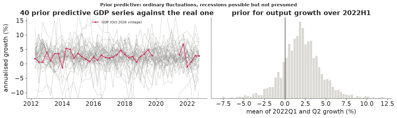
The prior puts quarterly output growth on roughly the scale of real GDP growth (a typical prior economy has a quarterly sd of 2.1 points against 1.5 for GDP in 2012-2019), allows much wilder ones, and does not rule a contraction in or out: about one chance in five that output fell over the first half of 2022, one in eight that both quarters were negative. These numbers are the baseline against which every posterior below should be read. Two quantities will carry the question from now on: P(both quarters negative), the two-quarter rule applied to latent output, and P(H1 contraction), the probability that output in 2022Q2 was below 2021Q4 (the mean of the two quarterly growth rates is negative).
C. GDP alone, 28 July 2022
The fitting machinery: swap in the readings, sample with nutpie (4 chains, 400 warm-up and 1,000 kept
draws each, the pm.sample defaults), then draw one exact latent path per posterior draw for 1,000 of
them.
ACTIVE_BASE = ["mu", "phi", "s", "sig_gdp"]


def active_vars(d):
    names = list(ACTIVE_BASE)
    if d["gdi_ok"].sum() > 0:
        names += ["sig_gdi"] + (["rho"] if d["rho_free"] > 0 else [])
    for k in MSER:
        if d[f"ic_{k}"].sum() > 0:
            names += [f"a_{k}", f"lam_{k}", f"sig_{k}"] + ([f"psi_{k}"] if d["use_ar"] > 0 else [])
    return names


def draw_paths(idata, d, n=1000, seed=0):
    """Exact draws of the latent path, one per posterior draw (n of them), plus those draws' parameters."""
    post = az.extract(idata, num_samples=n, random_seed=seed)
    P = {k: post[k].values for k in post.data_vars if post[k].ndim == 1}
    r = np.random.default_rng(seed)
    g = np.empty((n, T))
    for i in range(n):
        p = {k: v[i] for k, v in P.items()}
        Qd, b, _, _, _ = sensor_algebra(p, d, np)
        Qp = ar1_precision(p["phi"], p["s"]) + Qd
        L = np.linalg.cholesky(Qp)
        mean = np.linalg.solve(L.T, np.linalg.solve(L, b))
        g[i] = p["mu"] + mean + np.linalg.solve(L.T, r.standard_normal(T))
    return g, P


FITS = {}


def fit(key, vintage, seed, **kw):
    d = readings(vintage, **kw)
    t0 = time.time()
    idata = nutpie.sample(COMPILED.with_data(**d), chains=4, tune=400, draws=1000, seed=seed,
                          progress_bar=False, save_warmup=False)
    secs = time.time() - t0
    g, P = draw_paths(idata, d, seed=seed)
    gq = g @ A.T
    names = active_vars(d)
    rhat = max(float(az.rhat(idata.posterior[v]).max()) for v in names)
    ess = min(float(az.ess(idata.posterior[v]).min()) for v in names)
    div = int(idata.sample_stats["diverging"].sum())
    FITS[key] = {"idata": idata, "d": d, "g": g, "P": P, "gq": gq, "vintage": vintage,
                 "both": np.mean((gq[:, Q1] < 0) & (gq[:, Q2] < 0)),
                 "h1": np.mean(gq[:, [Q1, Q2]].mean(axis=1) < 0)}
    label = key if key.endswith(VLABEL[vintage]) else f"{key}, {VLABEL[vintage]}"
    print(f"{label:<28} {secs:3.0f} s, divergences {div}, max r_hat {rhat:.3f}, "
          f"min bulk ESS {ess:.0f} | 2022Q1 {gq[:, Q1].mean():+.2f} ± {gq[:, Q1].std():.2f}, "
          f"2022Q2 {gq[:, Q2].mean():+.2f} ± {gq[:, Q2].std():.2f} | P(both < 0) {FITS[key]['both']:.3f}, "
          f"P(H1 contraction) {FITS[key]['h1']:.3f}")
    return FITS[key]


f_gdp = fit("GDP alone", "2022-07-28", seed=RANDOM_SEED, sensors=("gdp",))
print(az.summary(f_gdp["idata"], var_names=ACTIVE_BASE, round_to=3).to_string())
GDP alone, Jul 2022            6 s, divergences 0, max r_hat 1.001, min bulk ESS 2560 | 2022Q1 +1.38 ± 1.05, 2022Q2 +1.00 ± 1.13 | P(both < 0) 0.047, P(H1 contraction) 0.104
          mean     sd  eti89_lb  eti89_ub  ess_bulk  ess_tail  r_hat  mcse_mean  mcse_sd
mu       2.212  0.321     1.699     2.733  9397.972  3038.865  1.001      0.003    0.006
phi      0.296  0.152     0.078     0.559  5168.182  2982.310  1.001      0.002    0.002
s        1.890  0.655     0.931     2.982  2560.122  2788.168  1.001      0.013    0.008
sig_gdp  1.139  0.334     0.577     1.649  2732.097  2128.925  1.001      0.006    0.005
The sampler is healthy (no divergences, r-hat 1.00, thousands of effective draws: integrating the path out removed the ridges). The answer may surprise anyone who took the two negative prints at face value: with GDP alone, the posterior mean of latent growth is about +1.4 in the first quarter and +1 in the second, and P(H1 contraction) is about 0.1 - lower than the prior's 0.19. Two things pull the estimate up from the prints. First, the history says growth averages about 2.2% ($\mu$) and that much of the quarter-to-quarter wobble in GDP is measurement noise. Second, both prints were fresh, so each carries 1.4 points of revision noise on top of $\sigma_P$. A reading of -1.6 with a standard deviation near 1.8 does not move a path that hovers around +2 very far.
What can one sensor learn about its own noise? Very little: GDP's variance is the sum of the economy's variance and the measurement noise, and a single series cannot split them except through the AR structure (smooth latent path, white noise).
fig, axes = plt.subplots(1, 2, figsize=(14, 4), width_ratios=[1.6, 1])
ax = axes[0]
gq = f_gdp["gq"]
lo, med, hi = np.quantile(gq, [0.055, 0.5, 0.945], axis=0)
qwin = QUARTERS >= "2016-01-01"
ax.fill_between(QUARTERS[qwin], lo[qwin], hi[qwin], color=RED, alpha=0.2, label="latent output growth, 89%")
ax.plot(QUARTERS[qwin], med[qwin], color=RED, lw=1.5)
ax.plot(QUARTERS[qwin], q0["gdp"][qwin], "o", color=INK, ms=4, label="GDP as of 28 Jul 2022")
ax.axhline(0, color=INK, lw=0.6)
ax.axvspan(pd.Timestamp("2019-12-01"), pd.Timestamp("2021-05-01"), color=LIGHT, alpha=0.6, lw=0)
ax.text(pd.Timestamp("2020-08-15"), 8.5, "masked", ha="center", fontsize=8, color=MUTED)
ax.set(ylim=(-5, 10), ylabel="annualised growth (%)", title="GDP alone: latent quarterly growth, 28 July 2022")
ax.legend(fontsize=8, loc="upper left")
ax = axes[1]
xs = np.linspace(0.01, 3.5, 300)
ax.plot(xs, stats.lognorm(0.5, scale=1.0).pdf(xs), color=MUTED, lw=1.5, label="prior")
ax.hist(f_gdp["idata"].posterior["sig_gdp"].values.ravel(), bins=60, density=True, color=RED, alpha=0.5,
        label="posterior, GDP alone")
ax.set(xlabel=r"$\sigma_P$, mature GDP measurement error (pp)", yticks=[],
       title="what GDP alone learns about its own noise")
ax.legend(fontsize=8);
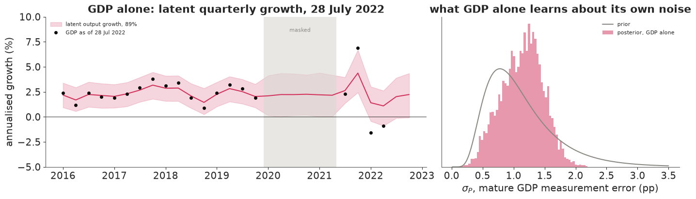
The latent band is wide - about ±1.2 points around each quarter before the pandemic and ±1.7 in 2022 - and in the masked quarters, where no sensor reports, the path simply returns to the long-run mean. The posterior for $\sigma_P$ (mean 1.1, sd 0.33) has moved only modestly from the prior (median 1, sd about 0.6), so the GDP-alone answer leans on that prior: how far the latent path follows the two negative prints depends on how noisy we believed GDP to be before seeing it. Fusion's first job is to let other sensors settle that instead.
D. Fusion, and a sensor that counts twice
Failure: errors that do not persist
The naive fused model takes all six sensors and treats each monthly sensor's error as independent from
month to month ($\psi_k = 0$, switched off through the use_ar data flag).
f_iid = fit("fused, iid errors", "2022-07-28", seed=RANDOM_SEED + 1, use_ar=0.0)
print(az.summary(f_iid["idata"], var_names=["mu", "phi", "s", "sig_gdp", "sig_gdi", "rho", "lam_payrolls",
                                            "sig_payrolls", "a_payrolls"], round_to=3).to_string())
fused, iid errors, Jul 2022   12 s, divergences 0, max r_hat 1.003, min bulk ESS 1472 | 2022Q1 +4.78 ± 0.55, 2022Q2 +3.69 ± 0.42 | P(both < 0) 0.000, P(H1 contraction) 0.000
               mean     sd  eti89_lb  eti89_ub  ess_bulk  ess_tail  r_hat  mcse_mean  mcse_sd
mu            2.459  0.410     1.820     3.103  3298.873  2769.165  1.000      0.007    0.008
phi           0.862  0.068     0.738     0.952  2692.634  2646.153  1.001      0.001    0.001
s             0.526  0.134     0.343     0.762  1759.355  2269.849  1.002      0.003    0.002
sig_gdp       1.536  0.212     1.237     1.902  4984.688  3113.874  1.000      0.003    0.004
sig_gdi       1.836  0.227     1.511     2.230  4252.843  2605.180  1.001      0.004    0.004
rho           0.186  0.162    -0.083     0.439  4721.730  3073.295  1.001      0.002    0.003
lam_payrolls  0.987  0.196     0.716     1.322  1471.954  1738.330  1.001      0.005    0.004
sig_payrolls  0.569  0.079     0.439     0.691  3188.640  2270.317  1.002      0.001    0.001
a_payrolls   -0.318  0.485    -1.154     0.360  1542.100  1719.832  1.002      0.013    0.010
The probability of a contraction has gone to zero, and the estimate of first-quarter growth is near +4.8 with a standard deviation around 0.55: the model is sure the economy was booming. Look at how it got there. The latent path became smooth (monthly persistence $\phi \approx 0.86$, innovation sd $s \approx 0.5$, against 0.3 and 1.9 with GDP alone), the payroll loading is about 1 and the payroll noise only about 0.6 points: the model has decided that the economy is payrolls. Payroll growth is very smooth from month to month; with independent errors, the only way the model can explain a smooth sensor is a smooth economy that the sensor reads almost perfectly. Payrolls grew at 3.6% in the first half of 2022, so the economy must have grown fast.
Can a check see this? If the model is right, a sensor's standardised innovations - here simply $(x_{k,t} - a_k - \lambda_k g_t)/\sigma_k$ - are white noise. For each posterior draw (with its own latent path) we compute their lag-1 autocorrelation and compare it with the same statistic on white noise of the same length: a posterior predictive check with a realised discrepancy (Gelman, Meng & Stern 1996). A second, blunter check asks how far the two GDP prints of 2022 sit from each model's latent quarterly growth, in units of their measurement sd.
def innovation_check(f, k, rng):
    """Lag-1 autocorrelation of standardised innovations: observed vs replicated, per posterior draw."""
    d, P, g = f["d"], f["P"], f["g"]
    ok = (d[f"ic_{k}"] > 0)
    x, xl = d[f"x_{k}"], d[f"xl_{k}"]
    psi = d["use_ar"] * P[f"psi_{k}"][:, None]
    e = x[None, :] - P[f"a_{k}"][:, None] - P[f"lam_{k}"][:, None] * g
    el = xl[None, :] - P[f"a_{k}"][:, None] - P[f"lam_{k}"][:, None] * np.c_[g[:, :1] * 0, g[:, :-1]]
    innov = (e - psi * el)[:, ok] / P[f"sig_{k}"][:, None]
    rep = rng.standard_normal(innov.shape)

    def ac1(z):
        z = z - z.mean(axis=1, keepdims=True)
        return (z[:, 1:] * z[:, :-1]).sum(axis=1) / (z**2).sum(axis=1)
    return ac1(innov), ac1(rep)


rows = []
for k in MSER:
    obs_ac, rep_ac = innovation_check(f_iid, k, rng)
    rows.append({"sensor": MNAME[k], "observed lag-1 autocorr (mean)": obs_ac.mean(),
                 "replicated (mean)": rep_ac.mean(), "P(replicated > observed)": np.mean(rep_ac > obs_ac)})
print("naive fused model, 28 July 2022:")
print(pd.DataFrame(rows).set_index("sensor").round(3).to_string())


def gdp_z(f, qi):
    """Posterior mean of (GDP print - latent growth) / measurement sd for quarter qi."""
    v = f["P"]["sig_gdp"] ** 2 + TAU["gdp"] ** 2 * f["d"]["fresh"][qi]
    return np.mean((f["d"]["gdp_y"][qi] - f["gq"][:, qi]) / np.sqrt(v))


print("\nGDP prints minus latent growth, in measurement sds:")
for f, lab in ((f_gdp, "GDP alone"), (f_iid, "fused, iid errors")):
    print(f"  {lab:<20} 2022Q1 {gdp_z(f, Q1):+.2f}, 2022Q2 {gdp_z(f, Q2):+.2f}")
naive fused model, 28 July 2022:
                            observed lag-1 autocorr (mean)  replicated (mean)  P(replicated > observed)
sensor
payrolls                                            -0.055             -0.009                     0.642
industrial production                                0.029             -0.008                     0.343
real income less transfers                          -0.125             -0.014                     0.882
real retail sales                                   -0.246             -0.011                     0.993

GDP prints minus latent growth, in measurement sds:
  GDP alone            2022Q1 -1.62, 2022Q2 -1.02
  fused, iid errors    2022Q1 -3.05, 2022Q2 -2.20
The check flags retail sales clearly (lag-1 autocorrelation about -0.25; 99% of white-noise replicates are above it): a strong month tends to be followed by a weak one, a sawtooth that independent errors cannot produce. Real income shows a hint of the same sawtooth (-0.12, with 88% of replicates above it, not enough to flag on its own). The check does not flag payrolls (-0.05, well inside the replicates). That is the blind spot of a residual check on a latent model: the model has bent the latent path to payrolls, so payrolls' residuals around that path look like white noise. The evidence is in the other sensors. Under the naive model the first-quarter GDP print sits about 3 measurement sds below latent output, against 1.6 for GDP alone; GDP has become an outlier to a path drawn by payrolls.
Fix: persistent sensor errors
Give every monthly sensor an AR(1) error, $u_{k,t} = \psi_k u_{k,t-1} + \sigma_k\eta_{k,t}$. A persistent deviation of payrolls from output - a stretch in which hiring runs ahead of output - is now one slow-moving error, not a dozen independent confirmations that output grew.
f_ar = fit("fused", "2022-07-28", seed=RANDOM_SEED + 2)
print(az.summary(f_ar["idata"], var_names=active_vars(f_ar["d"]), round_to=3).to_string())
rows = []
for k in MSER:
    obs_ac, rep_ac = innovation_check(f_ar, k, rng)
    rows.append({"sensor": MNAME[k], "observed lag-1 autocorr (mean)": obs_ac.mean(),
                 "replicated (mean)": rep_ac.mean(), "P(replicated > observed)": np.mean(rep_ac > obs_ac)})
print("\nfused model with AR(1) sensor errors, 28 July 2022:")
print(pd.DataFrame(rows).set_index("sensor").round(3).to_string())

print(f"GDP print minus latent growth, in measurement sds (fused, AR(1) errors): "
      f"2022Q1 {gdp_z(f_ar, Q1):+.2f}, 2022Q2 {gdp_z(f_ar, Q2):+.2f}")
fused, Jul 2022               11 s, divergences 0, max r_hat 1.003, min bulk ESS 913 | 2022Q1 +3.19 ± 0.60, 2022Q2 +1.24 ± 0.73 | P(both < 0) 0.000, P(H1 contraction) 0.003
                          mean     sd  eti89_lb  eti89_ub  ess_bulk  ess_tail  r_hat  mcse_mean  mcse_sd
mu                       2.325  0.264     1.906     2.746  4927.847  2924.546  1.001      0.004    0.004
phi                      0.190  0.100     0.050     0.364  3689.902  2034.217  1.000      0.002    0.002
s                        1.548  0.399     0.962     2.207  1013.834  1137.659  1.002      0.012    0.009
sig_gdp                  1.356  0.194     1.062     1.680  3600.020  2478.367  1.000      0.003    0.004
sig_gdi                  1.820  0.238     1.474     2.238  3280.417  2679.240  1.000      0.004    0.004
rho                      0.126  0.177    -0.160     0.401  2732.161  2143.743  1.001      0.003    0.003
a_payrolls               1.368  0.664     0.368     2.431  1976.241  2092.008  1.001      0.015    0.014
lam_payrolls             0.486  0.139     0.305     0.739   913.291  1149.789  1.002      0.005    0.004
sig_payrolls             0.248  0.097     0.135     0.416  1947.185  1592.142  1.001      0.003    0.005
psi_payrolls             0.963  0.039     0.901     0.989  1570.988  1663.881  1.002      0.001    0.004
a_indpro                -0.730  0.957    -2.346     0.662  2193.840  2043.076  1.000      0.021    0.017
lam_indpro               0.778  0.340     0.319     1.394  1875.785  2162.179  1.000      0.008    0.007
sig_indpro               5.833  0.404     5.227     6.518  4605.399  2859.230  1.001      0.006    0.007
psi_indpro               0.051  0.100    -0.109     0.211  4804.889  2529.061  1.000      0.001    0.002
a_income_ex_transfers    0.625  1.195    -1.449     2.353  2613.921  2398.722  1.003      0.024    0.022
lam_income_ex_transfers  0.857  0.416     0.314     1.635  2215.046  2155.556  1.001      0.009    0.009
sig_income_ex_transfers  8.684  0.598     7.805     9.684  5012.102  2819.516  1.001      0.009    0.012
psi_income_ex_transfers -0.103  0.094    -0.250     0.046  5383.087  2793.866  1.002      0.001    0.002
a_retail_sales           0.324  0.876    -1.138     1.625  2691.892  2432.284  1.000      0.017    0.015
lam_retail_sales         0.627  0.301     0.235     1.181  2330.884  2508.827  1.000      0.006    0.007
sig_retail_sales         7.509  0.523     6.727     8.400  5496.173  2827.645  1.001      0.007    0.010
psi_retail_sales        -0.244  0.096    -0.400    -0.093  5137.967  3016.639  1.002      0.001    0.002

fused model with AR(1) sensor errors, 28 July 2022:
                            observed lag-1 autocorr (mean)  replicated (mean)  P(replicated > observed)
sensor
payrolls                                            -0.078             -0.009                     0.695
industrial production                               -0.006             -0.006                     0.498
real income less transfers                          -0.031             -0.013                     0.571
real retail sales                                   -0.076             -0.011                     0.713
GDP print minus latent growth, in measurement sds (fused, AR(1) errors): 2022Q1 -2.45, 2022Q2 -1.09
The payroll error persistence is estimated at $\psi \approx 0.96$ (89% interval 0.90-0.99), far from the zero the naive model assumed: payrolls' deviation from output is nearly a random walk, so they inform the model about changes in growth, not its level. That estimate sits against the prior's upper edge of 0.99; the cap is what keeps the payroll error stationary, and since the first reading of a run has variance $\sigma_k^2/(1-\psi_k^2)$, how much the payroll level says depends on where that cap is. Their loading halves (to about 0.5) and their innovation sd drops to about 0.25. Retail sales gets $\psi \approx -0.25$ and real income $-0.10$, the sawtooth the check found. The latent path is no longer smooth ($\phi \approx 0.2$, $s \approx 1.5$, close to the GDP-alone values), and the GDP and GDI noise are now learned from the data rather than the prior: $\sigma_P \approx 1.4$ and $\sigma_I \approx 1.8$ with posterior sds of about 0.2. The innovation check passes for every sensor, and the first-quarter GDP print is now about 2.5 sds below latent output - still a large miss, which part G comes back to.
The answer to the question did not change - the contraction probability is still essentially zero - but its size did: first-quarter growth is now about +3.2 (sd 0.6) instead of +4.8, and second-quarter growth about +1.2 (sd 0.7) instead of +3.7.
fig, axes = plt.subplots(1, 2, figsize=(14, 4.2), width_ratios=[1.6, 1])
ax = axes[0]
mwin = MONTHS >= "2021-07-01"
for f, c, lab in ((f_gdp, RED, "GDP alone"), (f_iid, MUTED, "fused, iid errors"), (f_ar, BLUE, "fused, AR(1) errors")):
    lo, med, hi = np.quantile(f["g"], [0.055, 0.5, 0.945], axis=0)
    ax.fill_between(MONTHS[mwin], lo[mwin], hi[mwin], color=c, alpha=0.18)
    ax.plot(MONTHS[mwin], med[mwin], color=c, lw=1.8, label=lab)
ax.plot(MONTHS[mwin], m0["payrolls"][mwin], "s", color=PURPLE, ms=4, label="payroll growth (raw)")
ax.axhline(0, color=INK, lw=0.6)
ax.set(ylabel="annualised growth (%)", title="latent monthly output growth, 28 July 2022 (89% bands)",
       xlim=(MONTHS[mwin][0], pd.Timestamp("2022-07-01")), ylim=(-8, 12))
ax.legend(fontsize=8, ncols=2)
ax = axes[1]
for f, c, lab in ((f_gdp, RED, "GDP alone"), (f_iid, MUTED, "fused, iid"), (f_ar, BLUE, "fused, AR(1)")):
    ax.hist(f["gq"][:, [Q1, Q2]].mean(axis=1), bins=np.linspace(-4, 7, 70), density=True, color=c,
            alpha=0.45, label=f"{lab}: P(H1 contraction) = {f['h1']:.2f}")
ax.axvline(0, color=INK, lw=1)
ax.set(xlabel="mean growth of 2022Q1 and Q2 (%)", yticks=[], title="output growth over the first half of 2022")
ax.legend(fontsize=8)
for f, lab in ((f_gdp, "GDP alone"), (f_iid, "fused, iid"), (f_ar, "fused, AR(1)")):
    h1 = f["gq"][:, [Q1, Q2]].mean(axis=1)
    print(f"{lab:<13} first-half growth: mean {h1.mean():+.2f}, sd {h1.std():.2f}");
GDP alone     first-half growth: mean +1.19, sd 0.90
fused, iid    first-half growth: mean +4.23, sd 0.46
fused, AR(1)  first-half growth: mean +2.21, sd 0.54
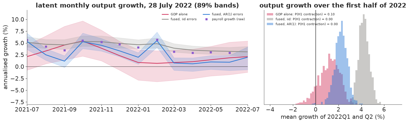
The left panel shows the failure: the iid model's latent path (grey) is a smoothed copy of payroll growth (purple squares). With persistent errors (blue) the path follows the month-to-month changes in payrolls (it jumps where payroll growth jumps, in late 2021 and early 2022) but not their level, and its band is about half as wide as the GDP-alone band (red). The right panel is our question, and the first visible effect of fusion: the GDP-alone posterior for first-half growth is wide (sd 0.9) and puts about a tenth of its mass below zero; the fused posterior is 40% narrower (sd 0.55) and sits entirely above zero.
E. Replaying the call
Now we repeat both fits - GDP alone, and fused with AR(1) errors - at the five later vintages. Nothing in the model changes; only the readings do.
for i, v in enumerate(VINTAGES[1:]):
    fit(f"GDP alone {VLABEL[v]}", v, seed=RANDOM_SEED + 10 + i, sensors=("gdp",))
    fit(f"fused {VLABEL[v]}", v, seed=RANDOM_SEED + 20 + i)
FITS["GDP alone Jul 2022"], FITS["fused Jul 2022"] = f_gdp, f_ar
GDP alone Aug 2022 6 s, divergences 0, max r_hat 1.001, min bulk ESS 2628 | 2022Q1 +1.48 ± 1.11, 2022Q2 +1.08 ± 1.10 | P(both < 0) 0.032, P(H1 contraction) 0.087
fused Aug 2022 12 s, divergences 0, max r_hat 1.002, min bulk ESS 937 | 2022Q1 +3.21 ± 0.59, 2022Q2 +1.21 ± 0.65 | P(both < 0) 0.000, P(H1 contraction) 0.000
GDP alone Sep 2022 6 s, divergences 0, max r_hat 1.001, min bulk ESS 2340 | 2022Q1 +0.57 ± 1.19, 2022Q2 +0.85 ± 1.22 | P(both < 0) 0.145, P(H1 contraction) 0.260
fused Sep 2022 12 s, divergences 0, max r_hat 1.005, min bulk ESS 880 | 2022Q1 +2.75 ± 0.62, 2022Q2 +1.28 ± 0.67 | P(both < 0) 0.001, P(H1 contraction) 0.003
GDP alone Oct 2023 6 s, divergences 0, max r_hat 1.003, min bulk ESS 2385 | 2022Q1 +0.23 ± 1.35, 2022Q2 +0.50 ± 1.09 | P(both < 0) 0.243, P(H1 contraction) 0.396
fused Oct 2023 11 s, divergences 0, max r_hat 1.004, min bulk ESS 912 | 2022Q1 +2.19 ± 0.68, 2022Q2 +0.58 ± 0.72 | P(both < 0) 0.002, P(H1 contraction) 0.018
GDP alone Oct 2024 6 s, divergences 0, max r_hat 1.001, min bulk ESS 2386 | 2022Q1 +0.86 ± 1.17, 2022Q2 +1.09 ± 0.99 | P(both < 0) 0.069, P(H1 contraction) 0.176
fused Oct 2024 10 s, divergences 0, max r_hat 1.008, min bulk ESS 950 | 2022Q1 +2.22 ± 0.60, 2022Q2 +1.17 ± 0.64 | P(both < 0) 0.000, P(H1 contraction) 0.003
GDP alone Oct 2026 6 s, divergences 0, max r_hat 1.003, min bulk ESS 2377 | 2022Q1 +0.88 ± 1.12, 2022Q2 +1.29 ± 0.88 | P(both < 0) 0.020, P(H1 contraction) 0.110
fused Oct 2026 10 s, divergences 0, max r_hat 1.003, min bulk ESS 968 | 2022Q1 +1.80 ± 0.57, 2022Q2 +1.20 ± 0.63 | P(both < 0) 0.003, P(H1 contraction) 0.006
rows = []
for v in VINTAGES:
    for kind in ("GDP alone", "fused"):
        f = FITS[f"{kind} {VLABEL[v]}"]
        rows.append({"vintage": VLABEL[v], "model": kind, "Q1 mean": f["gq"][:, Q1].mean(),
                     "Q1 sd": f["gq"][:, Q1].std(), "Q2 mean": f["gq"][:, Q2].mean(), "Q2 sd": f["gq"][:, Q2].std(),
                     "P(both < 0)": f["both"], "P(H1 contraction)": f["h1"]})
replay = pd.DataFrame(rows)
print(replay.round(3).to_string(index=False))
 vintage     model  Q1 mean  Q1 sd  Q2 mean  Q2 sd  P(both < 0)  P(H1 contraction)
Jul 2022 GDP alone    1.380  1.052    0.999  1.132        0.047              0.104
Jul 2022     fused    3.185  0.596    1.236  0.731        0.000              0.003
Aug 2022 GDP alone    1.476  1.107    1.079  1.097        0.032              0.087
Aug 2022     fused    3.212  0.587    1.211  0.648        0.000              0.000
Sep 2022 GDP alone    0.566  1.191    0.851  1.217        0.145              0.260
Sep 2022     fused    2.754  0.623    1.276  0.671        0.001              0.003
Oct 2023 GDP alone    0.231  1.354    0.499  1.087        0.243              0.396
Oct 2023     fused    2.192  0.681    0.584  0.720        0.002              0.018
Oct 2024 GDP alone    0.859  1.167    1.088  0.994        0.069              0.176
Oct 2024     fused    2.221  0.601    1.165  0.644        0.000              0.003
Oct 2026 GDP alone    0.876  1.120    1.292  0.883        0.020              0.110
Oct 2026     fused    1.803  0.573    1.195  0.635        0.003              0.006
fig, axes = plt.subplots(1, 3, figsize=(17, 4.6), width_ratios=[1.1, 1, 1])
x = np.arange(len(VINTAGES))
ax = axes[0]
for kind, c, mk in (("GDP alone", RED, "o"), ("fused", BLUE, "s")):
    pr = replay[replay.model == kind]["P(H1 contraction)"].to_numpy()
    ax.plot(x, pr, marker=mk, color=c, lw=2, ms=7, label=kind)
ax.axhline(0.2, color=INK, ls=":", lw=1)
ax.text(5.1, 0.205, "warning\nthreshold\n(part H)", fontsize=8, va="bottom", ha="right")
ax.set_xticks(x, [VLABEL[v] for v in VINTAGES], rotation=30)
ax.set(ylabel="P(output fell over 2022H1)", ylim=(-0.02, 0.6), title="the answer, vintage by vintage")
ax.legend(fontsize=9)
for ax, qi, qn in ((axes[1], Q1, "2022Q1"), (axes[2], Q2, "2022Q2")):
    for j, (kind, c) in enumerate((("GDP alone", RED), ("fused", BLUE))):
        lo, hi = [], []
        for v in VINTAGES:
            gqv = FITS[f"{kind} {VLABEL[v]}"]["gq"][:, qi]
            lo.append(np.quantile(gqv, 0.055)); hi.append(np.quantile(gqv, 0.945))
        mid = [FITS[f"{kind} {VLABEL[v]}"]["gq"][:, qi].mean() for v in VINTAGES]
        ax.errorbar(x + (j - 0.5) * 0.22, mid, yerr=[np.subtract(mid, lo), np.subtract(hi, mid)], fmt="os"[j],
                    color=c, capsize=3, lw=1.6, label=f"{kind}, 89% interval")
    ax.plot(x, tab_a[f"GDP {qn[-2:]}"], "x", color=RED, ms=9, mew=2, label="published GDP")
    ax.plot(x, tab_a[f"GDI {qn[-2:]}"], "+", color=BLUE, ms=11, mew=2, label="published GDI")
    ax.axhline(0, color=INK, lw=0.6)
    ax.set_xticks(x, [VLABEL[v] for v in VINTAGES], rotation=30)
    ax.set(title=f"latent growth in {qn}", ylabel="annualised growth (%)", ylim=(-3.5, 6))
    ax.legend(fontsize=7, loc="upper right")
fig.suptitle("GDP alone swings with every revision; the fused answer moves less and never comes near a contraction",
             fontsize=12);
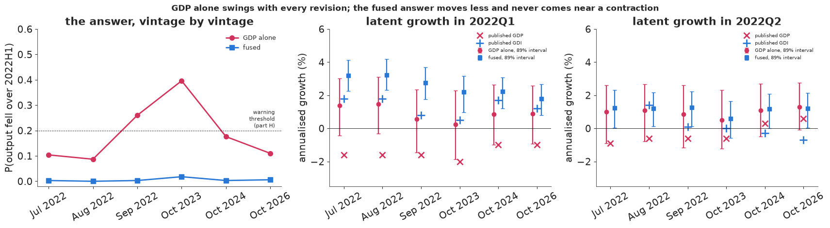
The left panel is the main result. With GDP alone, the probability that output fell over the first half of 2022 is about 0.1 in July and August 2022, about 0.26 after the September 2022 annual update and about 0.4 in October 2023, then back to 0.11-0.18 once the 2024 comprehensive revision lifted both quarters. The September jump is the model's own fresh/mature switch at work: the GDP prints barely changed (-1.6 and -0.6, as in August), but by the 245-day rule the first quarter stopped being fresh, so the model dropped its revision noise and trusted the same -1.6 more. The size of that jump is a property of our crude rule as much as of the data. October 2023 added a deeper first quarter (-2.0). The fused probability stays below 0.02 at every vintage.
The middle and right panels show the same story for each quarter. The GDP-alone intervals are 3-4 points wide and follow the GDP crosses; the fused intervals are about half as wide for 2022Q1 and about a third narrower for 2022Q2, and they sit above the GDP crosses and, for the first quarter in the 2022-2023 vintages, above the GDI pluses too - the monthly sensors pull them up. Across the six vintages the fused second-quarter estimate stays between about +0.6 and +1.3, while the GDP and GDI prints for that quarter cross zero in opposite directions.
But the fused first-quarter estimate did move, and in one direction: from about +3.2 in July 2022 to about +1.8 in October 2026. The July 89% interval, roughly +2.3 to +4.1, does not contain the October 2026 posterior mean. We return to this in part G.
F. Which sensor carries the answer?
Four more fits. The fused model without payrolls, as of July 2022. And GDP plus GDI with no monthly
sensors, as of August 2022 (when GDI first had a second-quarter reading), three times: with $\rho$ free,
and with $\rho$ fixed at 0 and at 0.8 through the rho_free / rho_value data switches.
fit("fused − payrolls", "2022-07-28", seed=RANDOM_SEED + 30,
    sensors=("gdp", "gdi", "indpro", "income_ex_transfers", "retail_sales"))
fit("GDP + GDI", "2022-08-25", seed=RANDOM_SEED + 31, sensors=("gdp", "gdi"))
for i, rho in enumerate((0.0, 0.8)):
    fit(f"GDP + GDI, rho={rho}", "2022-08-25", seed=RANDOM_SEED + 32 + i, sensors=("gdp", "gdi"), rho=rho)
f_gg = FITS["GDP + GDI"]
print(f"\nGDP + GDI, Aug 2022: posterior rho {f_gg['idata'].posterior['rho'].mean().item():+.2f} "
      f"± {f_gg['idata'].posterior['rho'].std().item():.2f} (prior sd 0.45); "
      f"fused, Jul 2022: {f_ar['idata'].posterior['rho'].mean().item():+.2f} ± "
      f"{f_ar['idata'].posterior['rho'].std().item():.2f}")
for key in ("GDP + GDI", "GDP + GDI, rho=0.0", "GDP + GDI, rho=0.8"):
    po = FITS[key]["idata"].posterior
    print(f"{key:<20} rho {float(po['rho'].mean()):+.2f}, sigma_P {float(po['sig_gdp'].mean()):.2f} "
          f"± {float(po['sig_gdp'].std()):.2f}, sigma_I {float(po['sig_gdi'].mean()):.2f} ± {float(po['sig_gdi'].std()):.2f}")
fused − payrolls, Jul 2022 9 s, divergences 0, max r_hat 1.005, min bulk ESS 1205 | 2022Q1 +1.98 ± 0.89, 2022Q2 +1.43 ± 1.03 | P(both < 0) 0.004, P(H1 contraction) 0.019
GDP + GDI, Aug 2022 6 s, divergences 0, max r_hat 1.001, min bulk ESS 1999 | 2022Q1 +1.54 ± 0.97, 2022Q2 +1.05 ± 1.01 | P(both < 0) 0.009, P(H1 contraction) 0.047
GDP + GDI, rho=0.0, Aug 2022 6 s, divergences 0, max r_hat 1.002, min bulk ESS 4275 | 2022Q1 +1.63 ± 0.94, 2022Q2 +1.09 ± 1.00 | P(both < 0) 0.017, P(H1 contraction) 0.047
GDP + GDI, rho=0.8, Aug 2022   7 s, divergences 0, max r_hat 1.008, min bulk ESS 261 | 2022Q1 +0.85 ± 1.24, 2022Q2 +0.57 ± 1.23 | P(both < 0) 0.122, P(H1 contraction) 0.248

GDP + GDI, Aug 2022: posterior rho -0.18 ± 0.32 (prior sd 0.45); fused, Jul 2022: +0.13 ± 0.18
GDP + GDI            rho -0.18, sigma_P 1.06 ± 0.29, sigma_I 1.64 ± 0.28
GDP + GDI, rho=0.0   rho +0.00, sigma_P 1.14 ± 0.24, sigma_I 1.71 ± 0.24
GDP + GDI, rho=0.8   rho +0.80, sigma_P 0.73 ± 0.63, sigma_I 2.52 ± 0.34
order = [("GDP alone", "GDP alone Jul 2022"), ("GDP + GDI (Aug)", "GDP + GDI"),
         ("GDP + GDI, ρ = 0 (Aug)", "GDP + GDI, rho=0.0"), ("GDP + GDI, ρ = 0.8 (Aug)", "GDP + GDI, rho=0.8"),
         ("GDP alone (Aug)", "GDP alone Aug 2022"), ("fused − payrolls", "fused − payrolls"),
         ("fused", "fused Jul 2022"), ("fused (Aug)", "fused Aug 2022")]
fig, axes = plt.subplots(1, 2, figsize=(14, 4.3), width_ratios=[1.3, 1])
ax = axes[0]
for j, (lab, key) in enumerate(order):
    h1 = FITS[key]["gq"][:, [Q1, Q2]].mean(axis=1)
    lo, q25, med, q75, hi = np.quantile(h1, [0.055, 0.25, 0.5, 0.75, 0.945])
    c = BLUE if "fused" in lab else (PURPLE if "GDI" in lab else RED)
    ax.plot([lo, hi], [j, j], color=c, lw=1.5)
    ax.plot([q25, q75], [j, j], color=c, lw=5)
    ax.plot(med, j, "o", color="white", mec=c, ms=6)
    ax.text(5.0, j, f"P = {FITS[key]['h1']:.3f}", va="center", fontsize=8)
ax.axvline(0, color=INK, lw=0.8)
ax.set_yticks(range(len(order)), [o[0] for o in order])
ax.invert_yaxis()
ax.set(xlim=(-3, 7.6), xlabel="mean growth of 2022Q1 and Q2 (%), 50% and 89% intervals",
       title="what each set of sensors says (July 2022 unless marked)")
ax = axes[1]
xs = np.linspace(-1, 1, 200)
ax.plot(xs, stats.beta(2, 2).pdf((xs + 1) / 2) / 2, color=MUTED, lw=1.5, label="prior")
for f, c, lab in ((f_gg, PURPLE, "GDP + GDI, Aug 2022"), (f_ar, BLUE, "fused, Jul 2022")):
    ax.hist(f["idata"].posterior["rho"].values.ravel(), bins=60, range=(-1, 1), density=True, color=c,
            alpha=0.45, label=lab)
ax.set(xlabel=r"$\rho$, correlation of GDP and GDI measurement errors", yticks=[],
       title="the GDP-GDI error correlation");
ax.legend(fontsize=8);
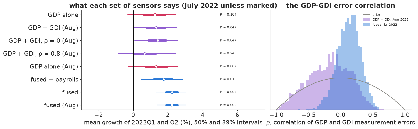
Reading the forest from the top. GDI matters once it exists: in August, GDP alone puts the probability of a first-half contraction at about 0.09, GDP plus GDI at about 0.05. The error correlation decides how much GDI counts. With $\rho = 0$ the answer is the same as with $\rho$ free (0.05), but with $\rho$ fixed at 0.8 it is about 0.25, worse than GDP alone. Two sensors with strongly correlated errors should rarely disagree by much, yet GDP and GDI differ with an sd of about 2 points; with $\rho = 0.8$ the model can only fit that gap by making GDI much noisier ($\sigma_I \approx 2.5$ against 1.6-1.7), so GDI is discounted and the latent growth estimate moves back towards the GDP prints and widens. The posterior for $\rho$ from GDP and GDI alone (right panel, purple) has a mean near -0.2 and an sd of 0.32 against the prior's 0.45: two series whose errors are both unobserved say little about how those errors co-move. The fused model, which has an independent view of output from the monthly sensors, narrows it to about 0.13 ± 0.18, a weak positive correlation.
Payrolls set the level: dropping them leaves the fused answer above zero (P about 0.02) but moves first-quarter growth from about +3.2 to +2.0 and widens it (sd 0.9 instead of 0.6). The monthly sensors carry the July call: before GDI's second-quarter number exists, the fused model is already as sure as it is in August.
G. Does the fused model fit, and was it right?
Posterior predictive check on GDP and GDI
Simulate GDP and GDI readings from the latest-vintage fused fit (latent path draw plus the bivariate measurement error) and compare with what was published.
f26 = FITS["fused Oct 2026"]
P26, gq26 = f26["P"], f26["gq"]
n_d = len(gq26)
z1, z2 = rng.standard_normal((2, n_d, NQ))
sp, si, rh = (P26[k][:, None] for k in ("sig_gdp", "sig_gdi", "rho"))
rep_gdp = gq26 + sp * z1
rep_gdi = gq26 + si * (rh * z1 + np.sqrt(1 - rh**2) * z2)
ok = ~np.isnan(q26["gdp"])
for s, rep in (("gdp", rep_gdp), ("gdi", rep_gdi)):
    lo, hi = np.quantile(rep, [0.055, 0.945], axis=0)
    inside = (q26[s] >= lo) & (q26[s] <= hi)
    pit = np.mean(rep < q26[s][None, :], axis=0)
    print(f"{s.upper()}: {inside[ok].mean():.0%} of {ok.sum()} quarters inside the 89% predictive interval; "
          f"PIT values: mean {pit[ok].mean():.2f}, sd {pit[ok].std():.2f} (uniform: 0.50, 0.29)")
gap = q26["gdp"] - q26["gdi"]
rep_gap = rep_gdp - rep_gdi
print(f"GDP - GDI gap: observed sd {np.nanstd(gap):.2f}; replicated sd {np.mean(np.std(rep_gap[:, ok], axis=1)):.2f} "
      f"(89%: {np.quantile(np.std(rep_gap[:, ok], axis=1), 0.055):.2f}-{np.quantile(np.std(rep_gap[:, ok], axis=1), 0.945):.2f})")
GDP: 92% of 37 quarters inside the 89% predictive interval; PIT values: mean 0.52, sd 0.26 (uniform: 0.50, 0.29)
GDI: 92% of 37 quarters inside the 89% predictive interval; PIT values: mean 0.49, sd 0.26 (uniform: 0.50, 0.29)
GDP - GDI gap: observed sd 2.06; replicated sd 2.08 (89%: 1.57-2.70)
A held-out GDP print
A sharper check: what did the other sensors predict for GDP in 2022Q1 and Q2 on 28 July 2022? We refit the fused model with those two GDP readings switched off (and with them GDI's first quarter, because the likelihood reads GDI given GDP), so that only the four monthly sensors speak for the first half of 2022, and ask what the fresh GDP prints, as published on 28 July, should have been (latent growth plus mature and revision noise). The tail probability of the published print is computed for each posterior draw exactly, from the normal measurement model, and then averaged; counting predictive draws below the print would rest on a handful of draws.
f_ho = fit("fused, GDP H1 hidden", "2022-07-28", seed=RANDOM_SEED + 40, hide=("2022-01-01", "2022-04-01"))
Pho = f_ho["P"]
sd_fresh = np.sqrt(Pho["sig_gdp"] ** 2 + TAU["gdp"] ** 2)
for qi, qn in ((Q1, "2022Q1"), (Q2, "2022Q2")):
    pred = f_ho["gq"][:, qi] + sd_fresh * rng.standard_normal(len(sd_fresh))
    p_low = stats.norm.cdf((q0["gdp"][qi] - f_ho["gq"][:, qi]) / sd_fresh)   # exact per draw, then averaged
    print(f"{qn}: predicted GDP print {pred.mean():+.2f}, 89% interval {np.quantile(pred, 0.055):+.2f} to "
          f"{np.quantile(pred, 0.945):+.2f}; published {q0['gdp'][qi]:+.1f}, "
          f"P(print this low or lower) = {p_low.mean():.4f}")
fused, GDP H1 hidden, Jul 2022  11 s, divergences 1, max r_hat 1.039, min bulk ESS 141 | 2022Q1 +4.32 ± 0.90, 2022Q2 +2.14 ± 0.90 | P(both < 0) 0.000, P(H1 contraction) 0.000
2022Q1: predicted GDP print +4.33, 89% interval +1.05 to +7.61; published -1.6, P(print this low or lower) = 0.0028
2022Q2: predicted GDP print +2.11, 89% interval -1.24 to +5.46; published -0.9, P(print this low or lower) = 0.0740
Scoring July 2022 against October 2026
for kind in ("GDP alone", "fused"):
    fj, fo = FITS[f"{kind} Jul 2022"], FITS[f"{kind} Oct 2026"]
    for qi, qn in ((Q1, "2022Q1"), (Q2, "2022Q2")):
        lo, hi = np.quantile(fj["gq"][:, qi], [0.055, 0.945])
        later = fo["gq"][:, qi].mean()
        avg_pub = (q26["gdp"][qi] + q26["gdi"][qi]) / 2
        print(f"{kind:<9} {qn}: July 2022 89% interval {lo:+.2f} to {hi:+.2f}; Oct 2026 posterior mean "
              f"{later:+.2f} ({'inside' if lo <= later <= hi else 'OUTSIDE'}); Oct 2026 mean of GDP and GDI "
              f"{avg_pub:+.2f} ({'inside' if lo <= avg_pub <= hi else 'OUTSIDE'})")
f_np26 = fit("fused − payrolls Oct 2026", "2026-10-01", seed=RANDOM_SEED + 41,
             sensors=("gdp", "gdi", "indpro", "income_ex_transfers", "retail_sales"))

fig, axes = plt.subplots(1, 2, figsize=(14, 4.2))
ax = axes[0]
qwin = QUARTERS >= "2014-01-01"
lo, hi = np.quantile(rep_gdp, [0.055, 0.945], axis=0)
ax.fill_between(QUARTERS[qwin], lo[qwin], hi[qwin], color=BLUE, alpha=0.2, label="replicated GDP, 89%")
ax.plot(QUARTERS[qwin], q26["gdp"][qwin], "o", color=RED, ms=4, label="GDP (Oct 2026)")
ax.plot(QUARTERS[qwin], q26["gdi"][qwin], "+", color=INK, ms=6, label="GDI (Oct 2026)")
ax.axvspan(pd.Timestamp("2019-12-01"), pd.Timestamp("2021-05-01"), color=LIGHT, alpha=0.6, lw=0)
ax.set(ylim=(-6, 10), ylabel="annualised growth (%)", title="fused fit, Oct 2026 vintage: posterior predictive")
ax.legend(fontsize=8, ncols=3, loc="upper left")
ax = axes[1]
bins = np.linspace(-5, 8, 80)
for kind, c in (("GDP alone", RED), ("fused", BLUE)):
    ax.hist(FITS[f"{kind} Jul 2022"]["gq"][:, Q1], bins=bins, density=True, histtype="step", color=c, lw=2,
            label=f"{kind}, Jul 2022")
    ax.hist(FITS[f"{kind} Oct 2026"]["gq"][:, Q1], bins=bins, density=True, color=c, alpha=0.25,
            label=f"{kind}, Oct 2026")
ax.axvline((q26["gdp"][Q1] + q26["gdi"][Q1]) / 2, color=INK, ls="--", lw=1, label="mean of GDP and GDI, Oct 2026")
ax.set(xlabel="latent growth in 2022Q1 (%)", yticks=[], title="2022Q1: what July 2022 thought vs what 2026 thinks")
ax.legend(fontsize=8);
GDP alone 2022Q1: July 2022 89% interval -0.43 to +3.02; Oct 2026 posterior mean +0.88 (inside); Oct 2026 mean of GDP and GDI +0.10 (inside)
GDP alone 2022Q2: July 2022 89% interval -0.89 to +2.62; Oct 2026 posterior mean +1.29 (inside); Oct 2026 mean of GDP and GDI -0.05 (inside)
fused     2022Q1: July 2022 89% interval +2.27 to +4.12; Oct 2026 posterior mean +1.80 (OUTSIDE); Oct 2026 mean of GDP and GDI +0.10 (OUTSIDE)
fused     2022Q2: July 2022 89% interval +0.04 to +2.31; Oct 2026 posterior mean +1.20 (inside); Oct 2026 mean of GDP and GDI -0.05 (OUTSIDE)
fused − payrolls Oct 2026 9 s, divergences 0, max r_hat 1.005, min bulk ESS 1000 | 2022Q1 +0.91 ± 0.78, 2022Q2 +0.82 ± 0.81 | P(both < 0) 0.028, P(H1 contraction) 0.067
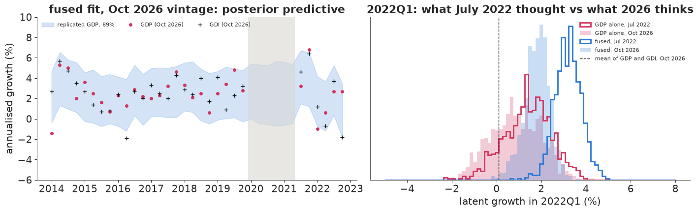
The fit. Over 2012-2022 (October 2026 vintage) the fused model's 89% predictive intervals contain 34 of 37 published GDP growth rates and 34 of 37 GDI ones, and the PIT values have the right centre with a slightly small spread (0.26 against 0.29 for a uniform), so the predictive intervals are, if anything, a little wide. The spread of the GDP-GDI gap is reproduced (2.06 observed, 2.08 replicated), which is what $\rho$, $\sigma_P$ and $\sigma_I$ must jointly get right.
The held-out prints. With their own GDP readings hidden, the monthly sensors as published in July 2022 put first-quarter growth at about +4.3 and expected the GDP print to be about +4.3 too (89%: +1.1 to +7.6). The probability of a print of -1.6 or lower, computed exactly for each posterior draw and averaged, is about 0.003, roughly one chance in 350; for the second-quarter -0.9 it is about 0.07. This fit mixed less well than the others - one divergence, r-hat up to about 1.04, bulk ESS about 140 - so read the first number as "a few in a thousand" rather than to its last digit. By the model's own account, then, the July 2022 data contained a conflict between GDP and the monthly sensors that its noise model does not expect. The fused posterior in part D resolved it largely in favour of the monthly sensors (+3.2 for the first quarter, much nearer their +4.3 than GDP's -1.6), with an interval only 2 points wide; the held-out check is the warning that this precision rests on a disagreement the model calls a 1-in-350 event.
The score. GDP alone in July 2022 was vague and therefore not wrong: its intervals contain both the October 2026 posterior and the October 2026 GDP-GDI average. The fused model in July 2022 was right about the sign but overconfident about the size: its first-quarter interval (+2.3 to +4.1) misses both the October 2026 fused posterior (+1.8) and the GDP-GDI average (+0.1), and its second-quarter interval misses the average narrowly. Hindsight sided partly with GDP: the monthly sensors that drove the July estimate were revised down (industrial production's first half from 5.1% to 0.9%, real income from +0.6% to -3.5%), and the model had treated them as final. The remaining gap between the 2026 fused estimate and the GDP-GDI average is mostly payrolls, which grew at about 3.5% a year in the first half at every vintage (3.4-3.7): without them, the October 2026 fit puts first-quarter growth at about +0.9 ± 0.8 instead of +1.8 ± 0.6. Fusion shrinks variance; it cannot remove a bias that the sensor models share.
H. Should a forecaster have called a recession?
Suppose a forecaster must decide, at each vintage, whether to issue a recession warning for the first half of 2022. A missed contraction is costly (clients are not hedged), a false warning less so; say a miss costs four times a false alarm. Warning when $P(\text{contraction}) > c_{\rm FA}/(c_{\rm FA} + c_{\rm miss}) = 1/5$ minimises expected cost.
dec = replay.pivot(index="vintage", columns="model", values="P(H1 contraction)").loc[[VLABEL[v] for v in VINTAGES]]
naive = ["warn" if (tab_a.loc[VLABEL[v], "GDP Q1"] < 0) and (tab_a.loc[VLABEL[v], "GDP Q2"] < 0) else "no"
         for v in VINTAGES]
dec["two negative GDP prints"] = naive
for kind in ("GDP alone", "fused"):
    dec[f"{kind}: decision"] = np.where(dec[kind] > 0.2, "warn", "no")
print(dec.round(3).to_string())
print(f"\nnotebook ran {time.time() - T_START:.0f} s")
model     GDP alone  fused two negative GDP prints GDP alone: decision fused: decision
vintage
Jul 2022      0.104  0.003                    warn                  no              no
Aug 2022      0.087  0.000                    warn                  no              no
Sep 2022      0.260  0.003                    warn                warn              no
Oct 2023      0.396  0.018                    warn                warn              no
Oct 2024      0.176  0.003                      no                  no              no
Oct 2026      0.110  0.006                      no                  no              no

notebook ran 212 s
The two-quarter rule, applied to GDP as published, says "warn" at every vintage until October 2024. GDP read as a noisy sensor says "no" in July and August 2022, "warn" after the September 2022 and 2023 updates, and "no" again from October 2024 - the decision flips twice because one noisy sensor is all it has. The fused model says "no" at every vintage, and that call held: the NBER never dated a recession, and in the October 2026 vintage GDP and GDI average to roughly zero growth over the half year, not a contraction. The decision-relevant gain from fusion is not a sharper number - part G showed the fused number was too high - but a stable answer, robust to which sensor gets revised next.
Summary
- Six sensors, one latent path. Monthly output growth as an AR(1), quarterly GDP and GDI as Mariano-Murasawa weighted sums of it with correlated errors, and four monthly indicators as affine noisy readings. The ragged edge and the masked pandemic months are just absent rows; GDP alone, GDP + GDI and the fused model are one compiled model with different sensors switched on.
- Integrating the path out with banded precision matrices (one 132 × 132 Cholesky per gradient) matched a brute-force multivariate normal on 508 readings to every printed digit. In prototypes not shown here, sampling the path directly gave r-hat 1.05-1.14 and ESS 20-90; the integrated fits ran in 6-12 seconds each with r-hat of 1.00-1.01 and almost no divergences, the fit with held-out GDP prints being the worst (r-hat about 1.04).
- Revision noise is large. A fresh GDP growth rate moved by 1.4 points (root mean square) on its way to the 2026 vintage, GDI by 1.5, over 22 quarters of 2014-2019. Monthly sensors were revised too: industrial production's first half of 2022 went from 5.1% to 0.9%.
- GDP alone, read as a noisy sensor, never said "contraction" with confidence - P(H1 contraction) about 0.1 in July 2022 against a prior 0.19 - but its answer swung between about 0.09 and 0.4 as GDP was revised, and it leans on the prior for GDP's own noise.
- The naive fused model was confidently wrong about the level (2022Q1 at +4.8 ± 0.55): payrolls with independent errors became a near-perfect reading of a smooth economy. A residual check flagged retail sales (with a hint of the same in real income) but not payrolls, whose residuals the bent path had made white; the 3-sd GDP misfit and the expanded model (payroll error persistence 0.96, interval 0.90-0.99) exposed it.
- Fusion changed the answer and kept it stable: P(H1 contraction) below 0.02 at all six vintages, against 0.09-0.4 for GDP alone, with intervals about half as wide for 2022Q1 and a third narrower for 2022Q2. But the July 2022 fused interval for 2022Q1 (+2.3 to +4.1) missed the 2026 estimate (+1.8): the monthly sensors it treated as final were revised down, and a held-out check had already put the GDP-monthly conflict at about 1 in 350. Most of the remaining gap to the GDP-GDI average (+0.1) is payrolls.
- The GDP-GDI error correlation is weakly identified from those two series alone (posterior sd 0.32 against a prior 0.45) and it matters: fixing it at 0.8 instead of 0 raised the August 2022 contraction probability from about 0.05 to 0.25. The monthly sensors pin it to about 0.13 ± 0.18.
- Decision: with a miss four times as costly as a false alarm, the fused model never warns; GDP alone warns at two of six vintages; the two-quarter rule warns at four. No recession was declared.
Try it yourself
- A recession regime. Replace the AR(1) mean by a two-state Markov-switching mean (expansion and contraction, as in Chauvet & Piger 2008), summed out with a forward filter as in E24. The integrated likelihood no longer applies exactly; sample the path non-centred or condition on the regime path. Does P(contraction regime in 2022H1) differ from P(H1 contraction) here, and is the regime model's prior probability of a recession more sensible?
- Revisions for every sensor. The monthly sensors are treated as final. Measure the revision noise of payrolls and real income from ALFRED vintages (as we did for GDP and GDI) and add it for readings less than a year old. Does the July 2022 fused interval for 2022Q1 now contain the 2026 estimate?
- A drifting long-run mean and a breaking sensor. Let $\mu$ follow a slow random walk by year (Antolin-Diaz, Drechsel & Petrella 2017) and let the payroll intercept $a_{\rm pay}$ change after the pandemic. Which of the two absorbs 2022's "jobs without output", and what happens to the fused level? While you are there, let the payroll error be a random walk ($\psi = 1$, payrolls informing only changes in growth) instead of an AR(1) capped at 0.99, and see how much of the payroll level effect survives.