The thesis of this notebook fits in one sentence: the Bayesian answer to a data problem is almost never a preprocessing step - it is another line in the model.
Deleting incomplete rows, filling holes with the column mean, trimming "outliers" and treating a published estimate as if it were the truth all feel like neutral housekeeping. None of them is. Each one is a modelling assumption made silently, in pandas, where no diagnostic can reach it:
| Housekeeping step | The assumption it makes |
|---|---|
drop rows with a NaN |
the rows that remain are a random sample of all rows |
| fill with the mean | the missing value is known exactly, and equals the mean |
| use a published rate as data | the rate was measured without error |
| delete the outlier | that point was generated by a process you need not describe |
Writing the assumption into the model costs a few lines. In return it becomes visible, checkable, and its uncertainty flows into every downstream number. D01 covers cleaning and encoding; this notebook starts where cleaning stops - with the holes and the noise that no amount of cleaning removes.
import logging
import warnings

import arviz as az
import matplotlib.pyplot as plt
import numpy as np
import pandas as pd
import pymc as pm
import pytensor.tensor as pt
from pymc.exceptions import ImputationWarning
from pymc_extras.marginal import marginalize, recover
from scipy import stats
from scipy.special import expit

from pymc_challenges import data

RANDOM_SEED = 2718
rng = np.random.default_rng(RANDOM_SEED)
az.style.use("arviz-variat")
logging.getLogger("pymc").setLevel(logging.ERROR)  # ~35 small fits below: keep the sampler log quiet

print(f"PyMC {pm.__version__}, ArviZ {az.__version__}")
PyMC 6.3.2, ArviZ 1.3.0
1 · Question and data
Gorman, Williams and Fraser measured three penguin species near Palmer Station, Antarctica, over three breeding seasons. Besides the familiar body measurements they took a blood sample from each bird, used to determine its sex (by DNA) and two stable-isotope ratios. One of them, $\delta^{15}$N, rises with trophic position: a bird that eats more fish and less krill has a higher value.
Within a species and sex, are birds that feed higher in the food web heavier or lighter? The regression is simple on purpose. The data problems are the subject.
A minimal inline clean (D01 does this properly, with range checks and assertions):
data.describe("penguins_raw")
raw = data.load("penguins_raw")

peng = pd.DataFrame({
    "species": raw["Species"].str.split().str[0],
    "year": pd.to_datetime(raw["Date Egg"]).dt.year,
    "mass": raw["Body Mass (g)"] / 1000,                      # kg
    "bill_depth": raw["Culmen Depth (mm)"],
    "male": raw["Sex"].map({"FEMALE": 0.0, "MALE": 1.0}),      # NaN stays NaN
    "d15n": raw["Delta 15 N (o/oo)"],
    "comment": raw["Comments"],
}).reset_index(drop=True)

SPECIES = ["Adelie", "Chinstrap", "Gentoo"]
YEARS = [2007, 2008, 2009]
X_REF = 8.7  # centre d15N here (close to its overall mean), so intercepts mean something

peng.head()
penguins_raw: 344 penguins as recorded in the field: messy column names, dates, comments, missing measurements.
  source: Gorman, Williams & Fraser (2014), Palmer Station LTER, via R `palmerpenguins` (raw field records).
  url:    https://vincentarelbundock.github.io/Rdatasets/csv/palmerpenguins/penguins_raw.csv
| species | year | mass | bill_depth | male | d15n | comment | |
|---|---|---|---|---|---|---|---|
| 0 | Adelie | 2007 | 3.75 | 18.7 | 1.0 | NaN | Not enough blood for isotopes. |
| 1 | Adelie | 2007 | 3.80 | 17.4 | 0.0 | 8.94956 | NaN |
| 2 | Adelie | 2007 | 3.25 | 18.0 | 0.0 | 8.36821 | NaN |
| 3 | Adelie | 2007 | NaN | NaN | NaN | NaN | Adult not sampled. |
| 4 | Adelie | 2007 | 3.45 | 19.3 | 0.0 | 8.76651 | NaN |
2 · Triage: how much is missing, where, and why?
Three questions before any modelling: how much, in which variables and rows, and is the missingness related to anything we did observe?
cols = ["mass", "bill_depth", "male", "d15n"]
missing = peng[cols].isna()
print(pd.DataFrame({"n missing": missing.sum(), "%": (100 * missing.mean()).round(1)}))
print(f"\nrows with at least one hole: {missing.any(axis=1).sum()} of {len(peng)}")

incomplete = peng[missing.any(axis=1)]
fig, ax = plt.subplots(figsize=(5, 6))
ax.imshow(incomplete[cols].isna(), aspect="auto", cmap="Greys", vmin=0, vmax=1.4)
ax.set_xticks(range(len(cols)), cols)
ax.set_yticks(range(len(incomplete)), [f"{r.species} {r.year} (row {i})" for i, r in incomplete.iterrows()],
              fontsize=8)
ax.set_title("Incomplete rows (dark = missing)");
            n missing    %
mass                2  0.6
bill_depth          2  0.6
male               11  3.2
d15n               14  4.1

rows with at least one hole: 20 of 344
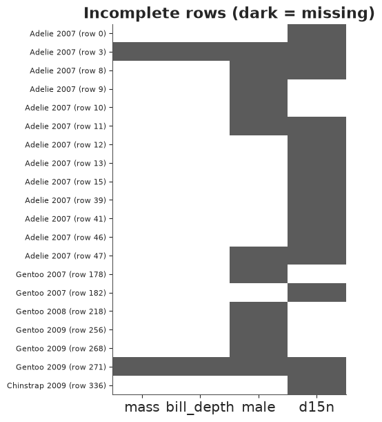
Few holes, but they are structured: two birds have nothing at all, the isotope holes are nearly all Adelies from 2007, and sex is missing for a different set of birds than $\delta^{15}$N. A complete-case analysis drops all 20 rows. Field data often says why a value is missing, and that is worth more than any statistical test:
print(incomplete.comment.value_counts().to_string())
print()
print(peng.assign(no_d15n=peng.d15n.isna()).groupby("year").no_d15n.agg(["sum", "size"])
      .rename(columns={"sum": "d15n missing", "size": "birds"}))
comment
Not enough blood for isotopes.                                          7
Sexing primers did not amplify.                                         4
No blood sample obtained.                                               2
No blood sample obtained for sexing.                                    2
Adult not sampled.                                                      1
Nest never observed with full clutch. Not enough blood for isotopes.    1
Sexing primers did not amplify. Not enough blood for isotopes.          1
Adult not sampled. Nest never observed with full clutch.                1
No delta15N data received from lab.                                     1

      d15n missing  birds
year
2007            12    110
2008             0    114
2009             2    120
"Not enough blood for isotopes", "sexing primers did not amplify", "adult not sampled": logistics and lab chemistry. Most isotope holes come from the first field season.
A plausible worry: a smaller bird yields less blood, so the outcome (mass) could drive the missingness of the covariate. That is a checkable statement - model the missingness indicator like any other binary outcome. Predictors: first season or not, and body mass standardised within species.
measured = peng.dropna(subset=["mass"]).reset_index(drop=True)   # the 2 empty rows cannot enter
d15n_missing = measured.d15n.isna().to_numpy().astype(int)
first_season = (measured.year == 2007).to_numpy().astype(float)
mass_z = measured.groupby("species").mass.transform(lambda s: (s - s.mean()) / s.std()).to_numpy()

with pm.Model() as triage_model:
    c0 = pm.Normal("intercept", -3, 2)            # missingness is rare: centre the prior near 5%
    c_first = pm.Normal("first_season", 0, 1.5)   # log-odds ratios beyond +-3 would be extreme
    c_mass = pm.Normal("mass_z", 0, 1.5)
    pm.Bernoulli("d15n_missing", logit_p=c0 + c_first * first_season + c_mass * mass_z,
                 observed=d15n_missing)
    triage_idata = pm.sample(random_seed=RANDOM_SEED, progressbar=False)

az.summary(triage_idata, ci_kind="hdi", ci_prob=0.94, round_to=2)
| mean | sd | hdi94_lb | hdi94_ub | ess_bulk | ess_tail | r_hat | mcse_mean | mcse_sd | |
|---|---|---|---|---|---|---|---|---|---|
| intercept | -4.72 | 0.60 | -5.84 | -3.67 | 1254.75 | 1344.74 | 1.0 | 0.02 | 0.01 |
| first_season | 2.34 | 0.66 | 1.15 | 3.63 | 1220.62 | 1315.39 | 1.0 | 0.02 | 0.01 |
| mass_z | 0.01 | 0.29 | -0.53 | 0.59 | 2352.07 | 2365.29 | 1.0 | 0.01 | 0.00 |
The first season raises the odds of a missing isotope value roughly tenfold ($e^{2.4} \approx 11$), while the coefficient of body mass is centred on zero - though with only 12 events its interval is wide, so "no evidence of" is all we can say. Missingness that depends on season matters only if $\delta^{15}$N itself differs between seasons:
peng.groupby(["species", "year"]).d15n.mean().unstack().round(2)
| year | 2007 | 2008 | 2009 |
|---|---|---|---|
| species | |||
| Adelie | 9.02 | 8.56 | 9.02 |
| Chinstrap | 9.12 | 9.44 | 9.56 |
| Gentoo | 7.97 | 8.42 | 8.27 |
It does, by up to half a unit - as much as the spread within a species and season. So any model for the missing values must know the season. That is the output of triage: not a verdict, but a list of variables the missing-data model has to condition on.
MCAR, MAR, MNAR - and what each one licenses
Write $R$ for the missingness indicator, $Y_\text{obs}$ for everything observed, $Y_\text{mis}$ for the values we do not have.
- MCAR (missing completely at random): $R$ is independent of everything, observed or not - a dropped test tube. The complete cases are a random subsample, so deleting rows is unbiased; it only wastes data. MCAR can be refuted from the data (we just did: season predicts $R$) but never confirmed.
- MAR (missing at random): $R$ depends only on things we observed - here season and perhaps mass. Given a model that conditions on those things, the missingness mechanism drops out of the likelihood ("ignorability") and the missing values are just more unknowns to integrate over. Deleting rows can now be biased - in a regression, whenever $R$ depends on the outcome - while a joint model is not.
- MNAR (missing not at random): $R$ depends on the missing value itself, even after conditioning on everything observed - the lab returns nothing above a detection range, heavy drinkers skip the alcohol question. The mechanism no longer drops out: you must model $R$ jointly with the data, and what identifies that model is an assumption that the data cannot check. MAR versus MNAR is never testable from the data at hand; it is argued from how the data were collected. "No blood sample obtained" is an argument for MAR.
3 · Missing outcomes: PyMC's automatic imputation
The easy case first. Two birds have no body mass. Hand PyMC an observed= array that
contains NaN (a NumPy array, a masked array or a pandas Series all behave the same) and it
splits the variable in two:
sp_all = pd.Categorical(peng.species, SPECIES).codes

with pm.Model(coords={"species": SPECIES, "bird": peng.index}) as outcome_model:
    a = pm.Normal("a", 4, 1, dims="species")
    sigma = pm.HalfNormal("sigma", 0.5)
    pm.Normal("mass", a[sp_all], sigma, observed=peng.mass, dims="bird")   # 2 NaN inside

print("free RVs      :", [v.name for v in outcome_model.free_RVs])
print("observed RVs  :", [v.name for v in outcome_model.observed_RVs])
print("deterministics:", [v.name for v in outcome_model.deterministics])
print("dims          :", outcome_model.named_vars_to_dims)
free RVs      : ['a', 'sigma', 'mass_unobserved']
observed RVs  : ['mass_observed']
deterministics: ['mass']
dims          : {'a': ('species',), 'mass': ('bird',)}
Read that output carefully, because it is all there is to "automatic imputation" in PyMC 6:
- an
ImputationWarningtells you it happened (from here on we silence it); mass_observedis the likelihood of the 342 measured values;mass_unobservedis a new free random variable with the same distribution, one element perNaN. It is sampled by NUTS like any parameter - and since it is continuous, the default nutpie sampler is perfectly happy;mass, the name you chose, is now aDeterministicthat stitches the two back together in the original row order. It is the only one that keeps yourdims; the two halves get anonymous dimensions such asmass_unobserved_dim_0. Usemassdownstream.
Two limitations: pm.Data refuses NaN, so an imputed variable cannot be swapped with
pm.set_data; and the pointwise log-likelihood (hence LOO) covers mass_observed only.
warnings.filterwarnings("ignore", category=ImputationWarning)

try:
    with pm.Model():
        pm.Data("mass", peng.mass.to_numpy())
except NotImplementedError as err:
    print("pm.Data with NaN ->", err)

with outcome_model:
    outcome_idata = pm.sample(random_seed=RANDOM_SEED, progressbar=False)

# the same model on the 342 complete rows
with pm.Model(coords={"species": SPECIES}) as dropped_model:
    a = pm.Normal("a", 4, 1, dims="species")
    sigma = pm.HalfNormal("sigma", 0.5)
    pm.Normal("mass", a[sp_all[peng.mass.notna()]], sigma, observed=peng.mass.dropna())
    dropped_idata = pm.sample(random_seed=RANDOM_SEED, progressbar=False)

pd.concat({
    "NaN in observed (344 rows)": az.summary(outcome_idata, var_names=["a", "sigma", "mass_unobserved"],
                                             round_to=3)[["mean", "sd", "r_hat"]],
    "rows dropped (342 rows)": az.summary(dropped_idata, var_names=["a", "sigma"], round_to=3)[["mean", "sd", "r_hat"]],
}, axis=1)
pm.Data with NaN -> Masked arrays or arrays with `nan` entries are not supported. Pass them directly to `observed` if you want to trigger auto-imputation
| NaN in observed (344 rows) | rows dropped (342 rows) | |||||
|---|---|---|---|---|---|---|
| mean | sd | r_hat | mean | sd | r_hat | |
| a[Adelie] | 3.701 | 0.037 | 1.001 | 3.701 | 0.037 | 1.000 |
| a[Chinstrap] | 3.733 | 0.057 | 1.001 | 3.734 | 0.055 | 1.002 |
| a[Gentoo] | 5.074 | 0.042 | 1.001 | 5.074 | 0.042 | 1.001 |
| sigma | 0.463 | 0.017 | 1.001 | 0.463 | 0.018 | 1.004 |
| mass_unobserved[0] | 3.706 | 0.464 | 1.000 | NaN | NaN | NaN |
| mass_unobserved[1] | 5.073 | 0.467 | 1.000 | NaN | NaN | NaN |
The parameters are the same to within Monte Carlo error, and they must be. A missing
outcome under MAR contributes the factor $\int p(y_\text{mis} \mid \theta)\,dy_\text{mis} = 1$
to the likelihood: it carries no information about the parameters. mass_unobserved is
simply the posterior predictive distribution for those two birds (an Adelie and a Gentoo:
compare their means with a, and their sd with sigma). Imputing outcomes is a
convenience for prediction and bookkeeping. It never rescues an analysis.
The same is not true of a missing covariate.
4 · A missing continuous covariate needs a model
The analysis model, for bird $i$ of species $s$ measured in season $t$:
$$ \text{mass}_i \sim \text{Normal}\big(\alpha_{s[i],\,t[i]} + \beta_\text{male}\,\text{male}_i + \beta_N\,(\delta^{15}\text{N}_i - 8.7),\ \sigma\big) $$
The intercept varies by species and season for a substantive reason that triage just handed us: the isotopic baseline of the food web shifts from year to year, so a difference in $\delta^{15}$N between seasons is not a difference in trophic position. $\beta_N$ should be a within-season comparison.
When $\delta^{15}$N$_i$ is missing, this likelihood term cannot be evaluated. Unlike a missing outcome it does not integrate to one: the row still holds a measured mass, which is informative about $\beta_N$ if we can say which values of $\delta^{15}$N are plausible for that bird. That statement is a model for the covariate, and triage told us what belongs in it - species, season and (looking at the group means) sex:
$$ \delta^{15}\text{N}_i \sim \text{Normal}\big(\mu_{s[i],\,t[i]} + \gamma\,\text{male}_i,\ \tau_{s[i]}\big) $$
In PyMC this is one extra line: give $\delta^{15}$N a distribution, pass the column with its
NaNs as observed=, and use the resulting variable in the regression. Each missing value
becomes a parameter whose posterior combines the covariate model (what do Adelies in 2007
look like?) with the outcome (what does this bird's mass suggest?).
Priors: intercepts Normal(4, 1) kg cover every penguin in the study; Normal(0, 0.5) kg per
unit of $\delta^{15}$N is generous, since the isotope spans about two units and mass varies
by a few hundred grams within a group. The helpers below are reused for the rest of part 1.
def design(d):
    """Index vectors for a penguin table: species code, season code, male indicator."""
    return (pd.Categorical(d.species, SPECIES).codes, pd.Categorical(d.year, YEARS).codes,
            d.male.to_numpy())


def penguin_priors():
    """Priors shared by every model of part 1 (call inside a model context)."""
    return {
        "mu_x": pm.Normal("mu_x", X_REF, 1.0, dims=("species", "year")),   # mean d15N, females
        "g_x": pm.Normal("g_x", 0, 0.5),                                   # male - female, d15N
        "s_x": pm.HalfNormal("s_x", 0.5, dims="species"),
        "a": pm.Normal("a", 4, 1, dims=("species", "year")),               # kg, female at d15N = 8.7
        "b_male": pm.Normal("b_male", 0, 1),
        "b_n": pm.Normal("b_n", 0, 0.5),                                   # kg per unit d15N
        "sigma": pm.HalfNormal("sigma", 0.5),
    }


def sexed_likelihood(p, d, d15n, suffix=""):
    """Covariate model + analysis model for birds of known sex. `d15n` may contain NaN."""
    sp, yr, male = design(d)
    x = pm.Normal("d15n" + suffix, p["mu_x"][sp, yr] + p["g_x"] * male, p["s_x"][sp], observed=np.asarray(d15n))
    pm.Normal("mass" + suffix, p["a"][sp, yr] + p["b_male"] * male + p["b_n"] * (x - X_REF), p["sigma"],
              observed=d.mass.to_numpy())
    return x


def fit_mass(d, d15n, selection=False, var_names=None, prior_only=False):
    """Fit the joint model to table `d` using the d15N column `d15n` (NaN = impute)."""
    with pm.Model(coords={"species": SPECIES, "year": YEARS}) as model:
        x = sexed_likelihood(penguin_priors(), d, d15n)
        if selection:  # section 6: model the missingness indicator as a function of the value itself
            c0 = pm.Normal("c0", 0, 2)
            c1 = pm.Normal("c1", 0, 3)
            pm.Bernoulli("is_missing", logit_p=c0 + c1 * (x - X_REF), observed=np.isnan(d15n).astype(int))
        if prior_only:
            return model, pm.sample_prior_predictive(500, random_seed=RANDOM_SEED)
        idata = pm.sample(random_seed=RANDOM_SEED, progressbar=False, var_names=var_names)
    return model, idata


STITCHED = {"mass", "d15n", "d15n_sexed"}   # observed + imputed, stitched together: mostly constants


def check(idata, label):
    """One-line sampler report: divergences, worst r_hat, smallest bulk ESS."""
    names = [v for v in idata.posterior.data_vars if v not in STITCHED]
    rhat = max(float(v.max()) for v in az.rhat(idata, var_names=names).data_vars.values())
    ess = min(float(v.min()) for v in az.ess(idata, var_names=names).data_vars.values())
    print(f"{label:<34} divergences {int(idata.sample_stats['diverging'].sum()):>2}   "
          f"max r_hat {rhat:.3f}   min ess_bulk {ess:,.0f}")


sexed = peng.dropna(subset=["mass", "male"]).reset_index(drop=True)
print(f"birds with mass and sex: {len(sexed)}, of which d15N missing: {sexed.d15n.isna().sum()}")

_, mass_prior = fit_mass(sexed, sexed.d15n.to_numpy(), prior_only=True)
prior_mass = mass_prior.prior_predictive["mass"]
print("prior predictive body mass, 3% / 50% / 97% quantiles (kg):",
      np.quantile(prior_mass, [0.03, 0.5, 0.97]).round(1))
birds with mass and sex: 333, of which d15N missing: 9
prior predictive body mass, 3% / 50% / 97% quantiles (kg): [1.2 3.9 6.7]
The prior predictive puts 94% of birds between roughly 1 and 7 kg: wider than the real range (2.7-6.3 kg), but penguin-sized. Now three ways to treat the missing isotope values, same model code each time:
- complete cases: drop the rows;
- mean-fill: replace each
NaNwith the column mean (df.fillna(df.mean())); - joint model: leave the
NaNs in and let the covariate model impute.
(With no NaN present the covariate model and the regression share no parameters, so the
extra line is harmless: the posterior of the regression is what it would be without it.)
complete = sexed.dropna(subset=["d15n"]).reset_index(drop=True)

real_fits = {
    "complete cases": fit_mass(complete, complete.d15n.to_numpy()),
    "mean-fill": fit_mass(sexed, sexed.d15n.fillna(sexed.d15n.mean()).to_numpy()),
    "joint model": fit_mass(sexed, sexed.d15n.to_numpy()),
}
for label, (_, idata) in real_fits.items():
    check(idata, f"{label} ({'324' if label == 'complete cases' else '333'} rows)")

full_model, full_idata = real_fits["complete cases"]   # reused below as the "truth" of the experiments


def coef_table(fits, var_names=("b_n", "b_male", "sigma")):
    """Posterior mean and sd of a few scalars for a dict of label -> idata."""
    out = {}
    for label, idata in fits.items():
        post = az.extract(idata, var_names=list(var_names))
        out[label] = {f"{v} {stat}": getattr(post[v], stat)().item() for v in var_names for stat in ("mean", "std")}
    return pd.DataFrame(out).T.round(3)


coef_table({k: v[1] for k, v in real_fits.items()})
complete cases (324 rows)          divergences  0   max r_hat 1.005   min ess_bulk 1,912
mean-fill (333 rows)               divergences  0   max r_hat 1.003   min ess_bulk 1,875
joint model (333 rows)             divergences  0   max r_hat 1.006   min ess_bulk 1,268
| b_n mean | b_n std | b_male mean | b_male std | sigma mean | sigma std | |
|---|---|---|---|---|---|---|
| complete cases | -0.203 | 0.058 | 0.703 | 0.035 | 0.311 | 0.012 |
| mean-fill | -0.181 | 0.057 | 0.690 | 0.035 | 0.313 | 0.012 |
| joint model | -0.204 | 0.060 | 0.696 | 0.036 | 0.312 | 0.012 |
All three agree to well within one posterior sd, and it would be dishonest to pretend otherwise: within a species, season and sex, a bird one unit higher in $\delta^{15}$N is about 0.2 kg lighter, whichever way the 9 holes are handled. When under 3% of a covariate is missing and the mechanism is benign, the method hardly matters. (Look closely, though: complete cases and the joint model agree to the third decimal, while nine mean-filled values were enough to pull the mean-fill estimate about 10% towards zero.) The joint model is still the one whose assumptions are on the page.
A quick posterior predictive check of the joint model before we lean on it:
joint_model, joint_idata = real_fits["joint model"]
with joint_model:
    pm.sample_posterior_predictive(joint_idata, var_names=["mass"], extend_inferencedata=True,
                                   random_seed=RANDOM_SEED, progressbar=False)
az.plot_ppc_dist(joint_idata, var_names=["mass"], num_samples=100);
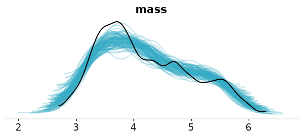
The broad shape with its heavy shoulder (Gentoos) is reproduced; the observed peak near 3.7 kg is a little sharper than in most replicates. Good enough for our purpose.
When it does matter: a controlled deletion experiment
To see the methods come apart we need more missingness and a less benign mechanism. Take the 324 complete birds - so that the full-data answer is known - and delete isotope values with the mechanism we worried about in triage: within its species and sex, a lighter bird is more likely to give too little blood.
$$P(\delta^{15}\text{N}_i \text{ missing}) = \text{logit}^{-1}(-0.3 - 1.5\, z_i), \qquad z_i = \text{mass standardised within species and sex}$$
This is MAR: mass is always observed. But the thing driving the missingness is the outcome of our regression.
z_within = complete.groupby(["species", "male"]).mass.transform(lambda s: (s - s.mean()) / s.std()).to_numpy()


def delete_mar(seed):
    """Boolean mask of deleted d15N values: lighter birds (within group) lose theirs more often."""
    return np.random.default_rng(seed).random(len(complete)) < expit(-0.3 - 1.5 * z_within)


deleted = delete_mar(RANDOM_SEED)
d15n_mar = complete.d15n.where(~deleted).to_numpy()
print(f"deleted {deleted.sum()} of {len(complete)} d15N values ({deleted.mean():.0%})")
print(f"mean mass: birds that kept their value {complete.mass[~deleted].mean():.2f} kg, "
      f"birds that lost it {complete.mass[deleted].mean():.2f} kg")

mar_fits = {
    "full data (the target)": full_idata,
    "complete cases": fit_mass(complete[~deleted].reset_index(drop=True), d15n_mar[~deleted])[1],
    "mean-fill": fit_mass(complete, np.where(deleted, np.nanmean(d15n_mar), d15n_mar))[1],
    "joint model": fit_mass(complete, d15n_mar)[1],
}
for label, idata in mar_fits.items():
    check(idata, label)
coef_table(mar_fits)
deleted 151 of 324 d15N values (47%)
mean mass: birds that kept their value 4.37 kg, birds that lost it 4.03 kg
full data (the target)             divergences  0   max r_hat 1.005   min ess_bulk 1,912
complete cases                     divergences  0   max r_hat 1.002   min ess_bulk 1,670
mean-fill                          divergences  0   max r_hat 1.005   min ess_bulk 3,377
joint model divergences 0 max r_hat 1.006 min ess_bulk 1,035
| b_n mean | b_n std | b_male mean | b_male std | sigma mean | sigma std | |
|---|---|---|---|---|---|---|
| full data (the target) | -0.203 | 0.058 | 0.703 | 0.035 | 0.311 | 0.012 |
| complete cases | -0.169 | 0.082 | 0.730 | 0.047 | 0.289 | 0.017 |
| mean-fill | -0.039 | 0.060 | 0.678 | 0.036 | 0.317 | 0.013 |
| joint model | -0.192 | 0.088 | 0.705 | 0.039 | 0.312 | 0.013 |
def interval_plot(ax, fits, var, truth_label=None, xlabel=None):
    """Posterior median with 50% and 94% intervals of scalar `var` for each fit."""
    for row, (label, idata) in enumerate(fits.items()):
        draws = az.extract(idata, var_names=var).values
        q = np.quantile(draws, [0.03, 0.25, 0.5, 0.75, 0.97])
        color = "k" if label == truth_label else f"C{row}"
        ax.plot(q[[0, 4]], [row, row], color=color, lw=1.5)
        ax.plot(q[[1, 3]], [row, row], color=color, lw=4)
        ax.plot(q[2], row, "o", color="w", mec=color, zorder=3)
        if label == truth_label:
            ax.axvline(q[2], color="k", ls=":", lw=1)
    ax.set_yticks(range(len(fits)), list(fits))
    ax.invert_yaxis()
    ax.set(xlabel=xlabel or var)


fig, ax = plt.subplots(figsize=(7, 3))
interval_plot(ax, mar_fits, "b_n", truth_label="full data (the target)", xlabel=r"$\beta_N$ (kg per unit $\delta^{15}$N)")
ax.axvline(0, color="grey", lw=0.8);
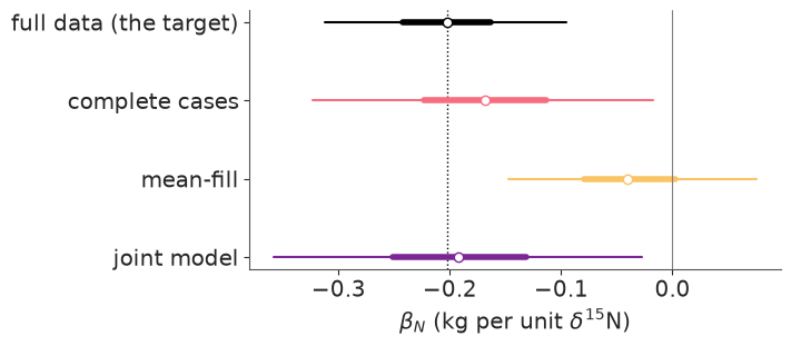
Read the table and the figure together (thick bar 50%, thin bar 94%, dotted line = the full-data posterior median that every method is trying to reproduce):
- Mean-fill is the worst offender. The filled-in value is wrong for every bird - an Adelie female and a Chinstrap male get the same number - so the covariate is polluted with noise that is unrelated to mass, and the slope is dragged towards zero. Worse, its posterior sd is about the same as with the full data: the model was told that the invented values are measurements, so it claims precision it does not have.
- Complete cases is honest about its uncertainty but selected on the outcome: lighter birds are under-represented in every group, which flattens the slope.
- The joint model sits closest to the target, with the widest interval of the three - the correct price for not knowing almost half of the covariate.
One deletion pattern is one draw from a random mechanism, and the differences above are not large compared with the posterior sd. Bias is a statement about the average over such draws, so repeat the deletion a few times. To keep the runtime sane only the joint model is refitted by MCMC; for the other two we use least squares, which with priors this weak is within rounding of the posterior mean (compare the first row with the table above).
dummies = pd.get_dummies(complete.species + complete.year.astype(str)).to_numpy(dtype=float)   # species x season


def ols_b_n(rows, d15n):
    """Least-squares coefficient of d15N in mass ~ species:season + male + d15N, using `rows`."""
    X = np.column_stack([dummies[rows], complete.male[rows], d15n[rows] - X_REF])
    return np.linalg.lstsq(X, complete.mass.to_numpy()[rows], rcond=None)[0][-1]


x_full = complete.d15n.to_numpy()
everyone = np.ones(len(complete), dtype=bool)
replicates = []
for rep in range(8):
    gone = deleted if rep == 0 else delete_mar(RANDOM_SEED + rep)
    x_rep = np.where(gone, np.nan, x_full)
    joint_rep = fit_mass(complete, x_rep, var_names=["b_n"])[1]
    replicates.append({
        "complete cases": ols_b_n(~gone, x_full),
        "mean-fill": ols_b_n(everyone, np.where(gone, np.nanmean(x_rep), x_full)),
        "joint model": float(joint_rep.posterior["b_n"].mean()),
    })
replicates = pd.DataFrame(replicates)
target = ols_b_n(everyone, x_full)

print(f"full-data estimate: {target:.3f}")
print(pd.DataFrame({"mean over 8 deletions": replicates.mean(), "sd": replicates.std()}).round(3))

fig, ax = plt.subplots(figsize=(7, 2.8))
for row, col in enumerate(replicates.columns):
    ax.plot(replicates[col], np.full(len(replicates), row) + rng.uniform(-0.12, 0.12, len(replicates)), "o",
            color=f"C{row + 1}", alpha=0.7)
    ax.plot(replicates[col].mean(), row, "|", color="k", ms=22, mew=2)
ax.axvline(target, color="k", ls=":", label="full-data estimate")
ax.set_yticks(range(3), replicates.columns)
ax.invert_yaxis()
ax.set(xlabel=r"estimate of $\beta_N$ in 8 independent deletions (bar = their mean)")
ax.legend(fontsize=8);
full-data estimate: -0.198
                mean over 8 deletions     sd
complete cases                 -0.160  0.054
mean-fill                      -0.038  0.042
joint model                    -0.216  0.064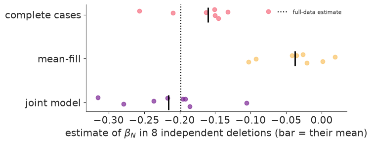
Eight replicates are few - each mean in the table has a standard error of about 0.02 - but the ranking is clear. The joint model is centred on the full-data answer to within that error; complete-case analysis loses about a fifth of the slope; mean-filling loses four fifths of it. (Do not read "towards zero" as a law for mean-filling: its bias depends on how the holes line up with the other predictors. With a mechanism that empties whole groups it can flip the sign of a coefficient - the second exercise.)
Because we deleted the values ourselves, we can also check the imputations against the truth - something you can never do with real missing data:
imputed = mar_fits["joint model"].posterior["d15n_unobserved"]
imp_mean = imputed.mean(("chain", "draw")).values
imp_lo, imp_hi = imputed.quantile([0.05, 0.95], dim=("chain", "draw")).values
truth = x_full[deleted]
covered = ((truth >= imp_lo) & (truth <= imp_hi)).mean()

fig, ax = plt.subplots(figsize=(5.5, 5))
sp_deleted = complete.species[deleted].to_numpy()
for k, name in enumerate(SPECIES):
    sel = sp_deleted == name
    ax.errorbar(truth[sel], imp_mean[sel], yerr=[imp_mean[sel] - imp_lo[sel], imp_hi[sel] - imp_mean[sel]],
                fmt="o", ms=3, lw=0.6, alpha=0.7, color=f"C{k}", label=name)
ax.axline((8.5, 8.5), slope=1, color="k", ls=":")
ax.set(xlabel=r"deleted (true) $\delta^{15}$N", ylabel="imputed: posterior mean and 90% interval",
       title=f"{covered:.0%} of 90% intervals contain the truth")
ax.legend();
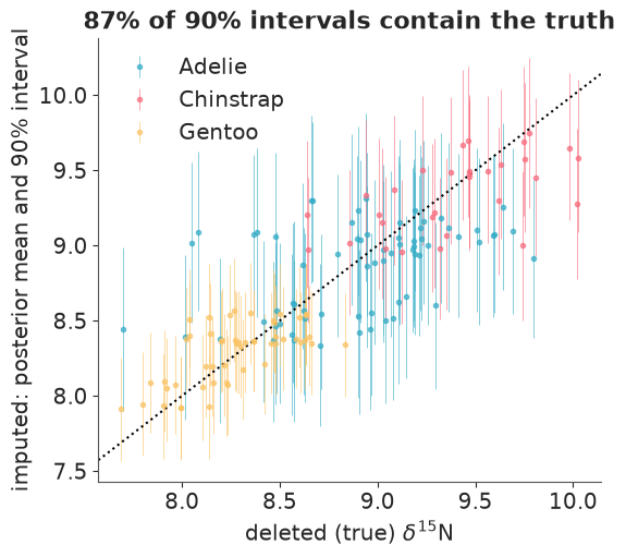
The point estimates track the truth only loosely - species and season carry most of the information, an individual's mass very little - and that is fine. Imputation is not about guessing the value; it is about carrying the right distribution for it, and the interval coverage says the distribution is about right. A filled-in mean is the same picture with every error bar set to zero.
5 · A missing discrete covariate: marginalise it
Sex is missing for 9 of the measured birds. Sex is not a nuisance here: males are about
0.7 kg heavier and feed slightly higher in the food web, so leaving it out would confound
$\beta_N$. The logic of section 4 applies unchanged - give sex a distribution,
$\text{male}_i \sim \text{Bernoulli}(\pi)$ - but the mechanics do not, because NUTS cannot
sample a discrete variable. Write the Bernoulli anyway and pm.sample quietly abandons
nutpie for PyMC's own CompoundStep of NUTS plus BinaryGibbsMetropolis. With 9 binary
unknowns that works; it mixes poorly when the discrete states are many or strongly coupled,
and every gradient-based tool (nutpie, JAX, ADVI, Pathfinder) is off the table.
The better route is the one from E04: sum the discrete variable out. For an unsexed bird the likelihood of what we did observe is a two-component mixture,
$$ p(x_i, y_i) = \sum_{s \in \{0, 1\}} \pi^s (1-\pi)^{1-s}\; p(x_i \mid s)\; p(y_i \mid x_i, s), $$
with $x$ = $\delta^{15}$N and $y$ = mass, and the posterior probability that bird $i$ is male
falls out of the same two terms by Bayes' rule. By hand this is a logsumexp inside a
pm.Potential. One wrinkle: 3 of the 9 unsexed birds have no isotope value either. Their
$x_i$ is a continuous unknown whose density is already inside the sum, so we declare it
pm.Flat - a placeholder that adds nothing to the log-density.
has_mass = peng.dropna(subset=["mass"])
unsexed = has_mass[has_mass.male.isna()]
sp_u, yr_u, _ = design(unsexed)
x_u_missing = unsexed.d15n.isna().to_numpy()
print(f"unsexed birds: {len(unsexed)}, of which without d15N: {x_u_missing.sum()}")

coords = {"species": SPECIES, "year": YEARS, "unsexed": unsexed.index, "unsexed_no_x": unsexed.index[x_u_missing]}

with pm.Model(coords=coords) as mixture_model:
    p = penguin_priors()
    pi = pm.Beta("p_male", 2, 2)

    # the 333 birds of known sex: exactly as before, plus sex itself as data for pi
    sexed_likelihood(p, sexed, sexed.d15n.to_numpy(), suffix="_sexed")
    pm.Bernoulli("male_sexed", pi, observed=sexed.male.to_numpy())

    # the 9 unsexed birds
    x_gap = pm.Flat("d15n_unsexed_missing", dims="unsexed_no_x")
    x_u = pt.set_subtensor(pt.as_tensor(unsexed.d15n.fillna(0.0).to_numpy())[x_u_missing], x_gap)

    def logp_if(s):
        """log [ p(sex = s) p(x | s) p(y | x, s) ] for every unsexed bird."""
        log_prior = pt.log(pi) if s == 1 else pt.log1p(-pi)
        x_dist = pm.Normal.dist(p["mu_x"][sp_u, yr_u] + p["g_x"] * s, p["s_x"][sp_u])
        y_dist = pm.Normal.dist(p["a"][sp_u, yr_u] + p["b_male"] * s + p["b_n"] * (x_u - X_REF), p["sigma"])
        return log_prior + pm.logp(x_dist, x_u) + pm.logp(y_dist, unsexed.mass.to_numpy())

    lp = pt.stack([logp_if(0), logp_if(1)])                       # shape (2, 9)
    pm.Potential("unsexed_loglik", pm.math.logsumexp(lp, axis=0).sum())
    pm.Deterministic("prob_male", pm.math.sigmoid(lp[1] - lp[0]), dims="unsexed")   # Bayes' rule, per draw

    mixture_idata = pm.sample(random_seed=RANDOM_SEED, progressbar=False)

check(mixture_idata, "hand-written mixture (342 rows)")
az.summary(mixture_idata, var_names=["b_n", "b_male", "g_x", "p_male", "sigma"], ci_kind="hdi", ci_prob=0.94,
           round_to=3)
unsexed birds: 9, of which without d15N: 3
hand-written mixture (342 rows) divergences 0 max r_hat 1.004 min ess_bulk 1,478
| mean | sd | hdi94_lb | hdi94_ub | ess_bulk | ess_tail | r_hat | mcse_mean | mcse_sd | |
|---|---|---|---|---|---|---|---|---|---|
| b_n | -0.202 | 0.060 | -0.309 | -0.084 | 1477.826 | 1861.018 | 1.003 | 0.002 | 0.001 |
| b_male | 0.701 | 0.035 | 0.633 | 0.766 | 2633.941 | 2990.067 | 1.000 | 0.001 | 0.000 |
| g_x | 0.135 | 0.028 | 0.084 | 0.189 | 2985.839 | 2883.748 | 1.001 | 0.001 | 0.000 |
| p_male | 0.497 | 0.027 | 0.445 | 0.546 | 7276.402 | 2721.626 | 1.002 | 0.000 | 0.000 |
| sigma | 0.312 | 0.012 | 0.290 | 0.336 | 7545.306 | 3139.762 | 1.000 | 0.000 | 0.000 |
Every measured bird is now in the model: 342 rows instead of the 324 complete cases. nutpie sampled it without complaint - there is nothing discrete left.
The same thing, automatically
pymc_extras.marginalize does the algebra for you. Write the model the generative way,
with a Bernoulli for the unknown sexes, and ask for it to be summed out; recover then
draws the sexes back, conditional on each posterior draw. Two practical findings from this
environment (pymc-extras 0.15): the automatic imputation of section 3 cannot sit downstream
of a marginalised variable (marginalize raises NotImplementedError on the boolean
indexing it generates), so the unsexed birds are split into those with and those without an
isotope value, and the missing isotope values are written as an ordinary latent pm.Normal.
with pm.Model(coords={"species": SPECIES, "year": YEARS}) as generative_model:
    p = penguin_priors()
    pi = pm.Beta("p_male", 2, 2)
    sexed_likelihood(p, sexed, sexed.d15n.to_numpy(), suffix="_sexed")
    pm.Bernoulli("male_sexed", pi, observed=sexed.male.to_numpy())

    for group, rows in [("with_x", unsexed[~x_u_missing]), ("no_x", unsexed[x_u_missing])]:
        sp_g, yr_g, _ = design(rows)
        male = pm.Bernoulli(f"male_{group}", pi, shape=len(rows))
        x_mu = p["mu_x"][sp_g, yr_g] + p["g_x"] * male
        if group == "with_x":
            x_g = pm.Normal(f"d15n_{group}", x_mu, p["s_x"][sp_g], observed=rows.d15n.to_numpy())
        else:
            x_g = pm.Normal(f"d15n_{group}", x_mu, p["s_x"][sp_g])          # latent, no data
        pm.Normal(f"mass_{group}", p["a"][sp_g, yr_g] + p["b_male"] * male + p["b_n"] * (x_g - X_REF), p["sigma"],
                  observed=rows.mass.to_numpy())

marginal_model = marginalize(generative_model, ["male_with_x", "male_no_x"])
with marginal_model:
    marginal_idata = pm.sample(random_seed=RANDOM_SEED, progressbar=False)
check(marginal_idata, "pymc_extras.marginalize")
recover(marginal_idata, model=marginal_model, random_seed=RANDOM_SEED)

recovered = np.concatenate([marginal_idata.posterior[f"male_{g}"].mean(("chain", "draw")).values
                            for g in ("with_x", "no_x")])
sex_table = pd.concat([unsexed[~x_u_missing], unsexed[x_u_missing]])[["species", "year", "mass", "bill_depth", "d15n"]]
sex_table["P(male) by hand"] = mixture_idata.posterior["prob_male"].mean(("chain", "draw")).to_series()
sex_table["P(male) marginalize + recover"] = recovered
print("b_n by hand: {:.3f}   marginalize: {:.3f}".format(
    float(mixture_idata.posterior["b_n"].mean()), float(marginal_idata.posterior["b_n"].mean())))
sex_table.round(2)
pymc_extras.marginalize divergences 0 max r_hat 1.004 min ess_bulk 1,506
b_n by hand: -0.202 marginalize: -0.205
| species | year | mass | bill_depth | d15n | P(male) by hand | P(male) marginalize + recover | |
|---|---|---|---|---|---|---|---|
| 9 | Adelie | 2007 | 4.25 | 20.2 | 9.13 | 0.98 | 0.98 |
| 10 | Adelie | 2007 | 3.30 | 17.1 | 8.63 | 0.02 | 0.02 |
| 178 | Gentoo | 2007 | 4.10 | 14.3 | 7.97 | 0.00 | 0.00 |
| 218 | Gentoo | 2008 | 4.65 | 14.4 | 8.24 | 0.03 | 0.03 |
| 256 | Gentoo | 2009 | 4.72 | 13.8 | 8.26 | 0.05 | 0.04 |
| 268 | Gentoo | 2009 | 4.88 | 15.7 | 8.04 | 0.05 | 0.04 |
| 8 | Adelie | 2007 | 3.48 | 18.1 | NaN | 0.18 | 0.18 |
| 11 | Adelie | 2007 | 3.70 | 17.3 | NaN | 0.48 | 0.49 |
| 47 | Adelie | 2007 | 2.98 | 18.9 | NaN | 0.01 | 0.01 |
The two routes agree to Monte Carlo accuracy. (The hand-written prob_male averages exact
probabilities; the recovered column averages 0/1 draws, so it is a little noisier.)
Check the imputed sexes against something the model never saw. Bill depth is strongly sexually dimorphic and was not used. Plot each unsexed bird among the sexed birds of its species:
prob_male = mixture_idata.posterior["prob_male"].mean(("chain", "draw")).to_series()

fig, axes = plt.subplots(1, 2, figsize=(9, 4))
for ax, name in zip(axes, ["Adelie", "Gentoo"]):
    known = sexed[sexed.species == name]
    for s, color, label in [(0, "C1", "female"), (1, "C0", "male")]:
        grp = known[known.male == s]
        ax.scatter(grp.mass, grp.bill_depth, s=10, color=color, alpha=0.35, label=label)
    who = unsexed[unsexed.species == name]
    sc = ax.scatter(who.mass, who.bill_depth, c=prob_male[who.index], cmap="coolwarm_r", vmin=0, vmax=1, s=90,
                    edgecolor="k", zorder=3)
    for i, r in who.iterrows():
        ax.annotate(f"{prob_male[i]:.2f}", (r.mass, r.bill_depth), textcoords="offset points", xytext=(7, 5),
                    fontsize=8)
    ax.set(title=name, xlabel="body mass (kg)", ylabel="bill depth (mm) - not in the model")
axes[0].legend(fontsize=8)
fig.colorbar(sc, ax=axes, label="posterior P(male)", shrink=0.8);
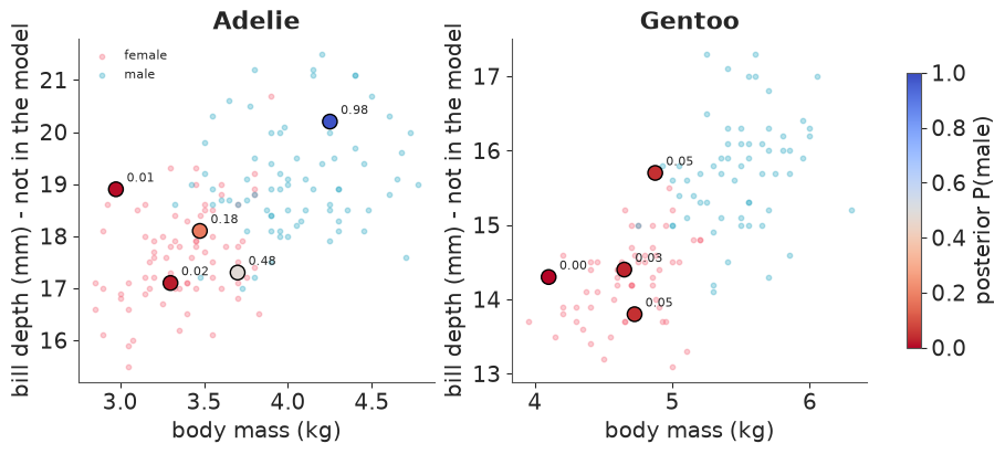
The large symbols are the unsexed birds, labelled with their posterior probability of being male. The probabilities follow body mass, as they must - mass is the only strongly dimorphic variable the model has - and bill depth mostly agrees: the one confident "male" has the deepest bill, the 50:50 bird sits where the clouds overlap. Two birds deserve a second look: the lightest Adelie and the heaviest unsexed Gentoo are called female with 95-99% confidence on mass alone, yet their bills are deep enough to sit among the males. The plot is telling you how to improve the model: give bill depth a sex-dependent likelihood too. That is one more line per measurement, and the third exercise below.
Did any of this change the answer?
part1 = {"complete cases (324 birds)": full_idata, "impute d15N (333 birds)": joint_idata,
         "+ marginalise sex (342 birds)": mixture_idata}
coef_table(part1)
| b_n mean | b_n std | b_male mean | b_male std | sigma mean | sigma std | |
|---|---|---|---|---|---|---|
| complete cases (324 birds) | -0.203 | 0.058 | 0.703 | 0.035 | 0.311 | 0.012 |
| impute d15N (333 birds) | -0.204 | 0.060 | 0.696 | 0.036 | 0.312 | 0.012 |
| + marginalise sex (342 birds) | -0.202 | 0.060 | 0.701 | 0.035 | 0.312 | 0.012 |
No - and with 20 incomplete rows out of 344, and mechanisms as benign as field logistics, it should not. That is a result: we now know the conclusion does not hinge on the dropped rows, which a complete-case analysis can only assume. The deletion experiment showed how quickly that changes when more is missing or the mechanism touches the outcome.
6 · MNAR: when the value causes its own absence
Everything so far assumed MAR. To make MNAR concrete, delete values with a mechanism that depends on the value itself: suppose the isotope lab fails more often on samples high in $\delta^{15}$ N,
$$P(\delta^{15}\text{N}_i \text{ missing}) = \text{logit}^{-1}\big(-0.5 + 2\,(\delta^{15}\text{N}_i - 8.7)\big).$$
The target this time is a descriptive one that this mechanism should damage: the mean $\delta^{15}$ N of each species among these 324 birds - which we know exactly.
def delete_mnar(seed):
    """Boolean mask of deleted d15N values: the higher the value, the likelier it is lost."""
    return np.random.default_rng(seed).random(len(complete)) < expit(-0.5 + 2.0 * (x_full - X_REF))


gone_mnar = delete_mnar(RANDOM_SEED + 100)
d15n_mnar = np.where(gone_mnar, np.nan, x_full)
print(f"deleted {gone_mnar.sum()} of {len(complete)} values ({gone_mnar.mean():.0%}); share deleted by species:")
print(pd.Series(gone_mnar).groupby(complete.species).mean().round(2).to_string())

mar_model, mar_idata = fit_mass(complete, d15n_mnar)                       # assumes MAR: ignores the mechanism
sel_model, sel_idata = fit_mass(complete, d15n_mnar, selection=True)      # models the mechanism
check(mar_idata, "MAR joint model")
check(sel_idata, "selection model")
print(az.summary(sel_idata, var_names=["c0", "c1"], ci_kind="hdi", ci_prob=0.94, round_to=2)
      [["mean", "sd", "hdi94_lb", "hdi94_ub"]])
coef_table({"full data": full_idata, "MAR joint model": mar_idata, "selection model": sel_idata})
deleted 133 of 324 values (41%); share deleted by species:
species
Adelie       0.48
Chinstrap    0.61
Gentoo       0.21
MAR joint model                    divergences  0   max r_hat 1.004   min ess_bulk 996
selection model                    divergences  0   max r_hat 1.006   min ess_bulk 955
    mean    sd  hdi94_lb  hdi94_ub
c0 -0.52  0.14     -0.79     -0.26
c1 1.97 0.31 1.41 2.59| b_n mean | b_n std | b_male mean | b_male std | sigma mean | sigma std | |
|---|---|---|---|---|---|---|
| full data | -0.203 | 0.058 | 0.703 | 0.035 | 0.311 | 0.012 |
| MAR joint model | -0.112 | 0.082 | 0.686 | 0.036 | 0.315 | 0.013 |
| selection model | -0.100 | 0.076 | 0.686 | 0.037 | 0.315 | 0.013 |
The selection model is the MAR model plus one line (see fit_mass): the missingness
indicator gets a Bernoulli likelihood whose logit depends on the completed covariate
vector - observed values where we have them, the latent imputations where we do not. The
imputations are now pulled by three things: the covariate model, the bird's mass, and the
fact that the value went missing.
sp_complete = complete.species.to_numpy()
true_means = pd.Series(x_full).groupby(sp_complete).mean()
observed_means = pd.Series(x_full[~gone_mnar]).groupby(sp_complete[~gone_mnar]).mean()

rows = {}
for label, idata in [("MAR joint model", mar_idata), ("selection model", sel_idata)]:
    completed = idata.posterior["d15n"].stack(sample=("chain", "draw")).values      # (bird, sample)
    for name in SPECIES:
        draws = completed[sp_complete == name].mean(axis=0)
        lo, hi = np.quantile(draws, [0.03, 0.97])
        rows[(name, label)] = {"estimate": draws.mean(), "3%": lo, "97%": hi}
mnar_table = pd.DataFrame(rows).T
mnar_table.insert(0, "true mean", [true_means[k[0]] for k in mnar_table.index])
mnar_table.insert(1, "mean of survivors", [observed_means[k[0]] for k in mnar_table.index])
mnar_table.round(3)
| true mean | mean of survivors | estimate | 3% | 97% | ||
|---|---|---|---|---|---|---|
| Adelie | MAR joint model | 8.859 | 8.724 | 8.767 | 8.711 | 8.826 |
| Chinstrap | MAR joint model | 9.356 | 9.109 | 9.212 | 9.124 | 9.305 |
| Gentoo | MAR joint model | 8.249 | 8.219 | 8.230 | 8.211 | 8.248 |
| Adelie | selection model | 8.859 | 8.724 | 8.890 | 8.820 | 8.965 |
| Chinstrap | selection model | 9.356 | 9.109 | 9.294 | 9.207 | 9.396 |
| Gentoo | selection model | 8.249 | 8.219 | 8.247 | 8.228 | 8.267 |
fig, axes = plt.subplots(1, 2, figsize=(9, 4.2), sharex=True, sharey=True)
for ax, (label, idata) in zip(axes, [("MAR joint model", mar_idata), ("selection model", sel_idata)]):
    imp = idata.posterior["d15n_unobserved"].mean(("chain", "draw")).values
    for k, name in enumerate(SPECIES):
        sel = sp_complete[gone_mnar] == name
        ax.scatter(x_full[gone_mnar][sel], imp[sel], s=12, alpha=0.7, color=f"C{k}", label=name)
    ax.axline((8.5, 8.5), slope=1, color="k", ls=":")
    ax.set_title(f"{label}\nmean error of imputations {np.mean(imp - x_full[gone_mnar]):+.2f}", fontsize=11)
    ax.set(xlabel=r"deleted (true) $\delta^{15}$N")
axes[0].set(ylabel="posterior mean imputation")
axes[0].legend(fontsize=8);
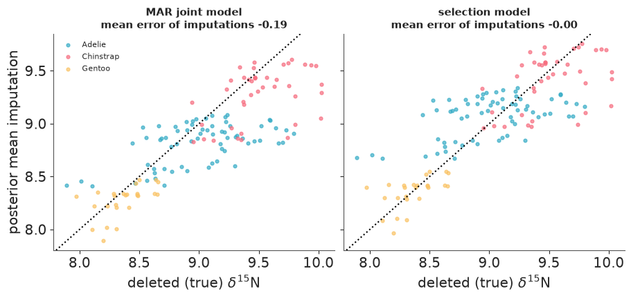
Under MNAR the MAR model is biased and confident: its imputations look like the
survivors, the survivors are the low values, and its 94% intervals for all three species
means miss the truth (Gentoo, which lost the fewest values, only just). The selection model
recovers the mechanism (c0, c1; we used -0.5 and 2), its imputations are unbiased on
average, and all three intervals now contain the true mean - with wider intervals, as they
should be.
Now the coefficient table. $\beta_N$ is the same in the two fits: modelling the mechanism did nothing for it, and in theory it did not need to, because selection on a covariate does not bias a correctly specified regression on that covariate. MNAR damages what the mechanism points at. Yet both estimates are only half the full-data value. How much of that is bad luck in one deletion? Least squares on the survivors, repeated 500 times, answers in milliseconds:
cc_slopes = np.array([ols_b_n(~delete_mnar(k), x_full) for k in range(500)])
print(f"complete-case slope over 500 MNAR deletions: mean {cc_slopes.mean():.3f}, sd {cc_slopes.std():.3f}   "
      f"(this deletion: {ols_b_n(~gone_mnar, x_full):.3f}, full data: {target:.3f})")
complete-case slope over 500 MNAR deletions: mean -0.145, sd 0.053 (this deletion: -0.103, full data: -0.198)
Mostly luck - this deletion sits almost one sd on the unlucky side - plus a smaller systematic part: on average the survivors give about three quarters of the full-data slope. "Selection on a covariate is harmless" holds for a correctly specified regression, and real penguins are not exactly linear in $\delta^{15}$N: remove the high values and the best-fitting line changes. No missing-data method repairs that; it is ordinary model misspecification, made visible by the deletion.
Before filing this under "solved", be clear about where the identification comes from, because the data cannot verify any of it:
- the shape assumptions - $\delta^{15}$N is Normal within a group, the mechanism is logistic-linear. A selection model reads skewness in the observed values as evidence of selection. If the true distribution were skewed, it would "correct" a bias that is not there;
- an exclusion restriction - species, season, sex and mass predict $\delta^{15}$N but are
assumed to affect missingness only through it. The very different deletion rates across
species are what pin down
c1.
We generated the data this way, so the model is right by construction. With real MNAR data
you would not know, and the honest workflow is a sensitivity analysis: fix c1 at a few
plausible values and report how far the conclusions move.
7 · Measurement error: when the data are themselves estimates
New data, same idea. The divorce and marriage rates of the US states are survey estimates, published with standard errors. A textbook regression treats 50 numbers of very different quality as equally exact.
data.describe("waffle_divorce")
waffle = data.load("waffle_divorce")
waffle[["Location", "Population", "MedianAgeMarriage", "Marriage", "Marriage SE", "Divorce", "Divorce SE"]] \
    .sort_values("Population").iloc[[0, 1, 2, -3, -2, -1]]
waffle_divorce: Divorce and marriage rates for 50 US states WITH their standard errors, plus median age at marriage.
  source: US Census / American Community Survey state statistics, via McElreath's `rethinking`.
  url:    https://raw.githubusercontent.com/rmcelreath/rethinking/master/data/WaffleDivorce.csv
| Location | Population | MedianAgeMarriage | Marriage | Marriage SE | Divorce | Divorce SE | |
|---|---|---|---|---|---|---|---|
| 49 | Wyoming | 0.56 | 24.2 | 30.7 | 3.92 | 10.3 | 1.90 |
| 8 | District of Columbia | 0.60 | 29.7 | 17.7 | 2.53 | 6.3 | 1.89 |
| 44 | Vermont | 0.63 | 26.9 | 16.4 | 2.40 | 9.6 | 1.87 |
| 31 | New York | 19.38 | 28.4 | 16.8 | 0.47 | 6.6 | 0.31 |
| 42 | Texas | 25.15 | 25.2 | 21.5 | 0.61 | 10.0 | 0.35 |
| 4 | California | 37.25 | 26.8 | 19.1 | 0.39 | 8.0 | 0.24 |
fig, ax = plt.subplots(figsize=(6, 4))
ax.scatter(waffle.Population, waffle["Divorce SE"], label="divorce rate")
ax.scatter(waffle.Population, waffle["Marriage SE"], marker="s", alpha=0.6, label="marriage rate")
ax.set(xscale="log", yscale="log", xlabel="population (millions)", ylabel="standard error (per 1000 adults)")
ax.legend()
print(f"Divorce SE ranges from {waffle['Divorce SE'].min()} to {waffle['Divorce SE'].max()}; "
      f"the sd of the divorce rates themselves is {waffle.Divorce.std():.2f}")
Divorce SE ranges from 0.24 to 2.5; the sd of the divorce rates themselves is 1.82
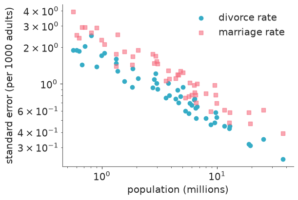
The standard errors fall with population like $1/\sqrt{n}$ and span a factor of ten. For South Dakota, Alaska or Wyoming the error is as large as the whole between-state spread; for California it is negligible.
Does a state's divorce rate depend on its marriage rate, once median age at marriage is accounted for? (McElreath's running example, Statistical Rethinking ch. 5 and 15. We standardise all three variables, and the standard errors with them.)
The measurement-error model adds one layer. The regression is about the true rate, which is latent; the published rate is a noisy reading of it with known sd:
$$ \begin{aligned} D^\text{true}_i &\sim \text{Normal}(\alpha + \beta_A A_i + \beta_M M_i,\ \sigma) \\ D^\text{obs}_i &\sim \text{Normal}(D^\text{true}_i,\ \text{SE}_i) \end{aligned} $$
Error in a predictor is handled the same way, and as in section 4 the latent predictor needs a distribution of its own - a covariate model. Marriage rate and age at marriage are strongly correlated (-0.72), so that model conditions on age: $M^\text{true}_i \sim \text{Normal}(\gamma_0 + \gamma_A A_i, \tau)$, $M^\text{obs}_i \sim \text{Normal}(M^\text{true}_i, \text{SE}^M_i)$.
def standardize(s):
    return ((s - s.mean()) / s.std()).to_numpy()


D_obs, M_obs, A = standardize(waffle.Divorce), standardize(waffle.Marriage), standardize(waffle.MedianAgeMarriage)
D_se = (waffle["Divorce SE"] / waffle.Divorce.std()).to_numpy()
M_se = (waffle["Marriage SE"] / waffle.Marriage.std()).to_numpy()
STATES = waffle.Loc.to_numpy()


def fit_divorce(error_in=(), likelihood="normal", keep=None, nu=None):
    """Divorce ~ age + marriage. error_in: subset of {"D", "M"}; likelihood: "normal" or "student"."""
    keep = np.ones(len(waffle), dtype=bool) if keep is None else keep
    with pm.Model(coords={"state": STATES[keep]}) as model:
        a = pm.Normal("a", 0, 0.2)
        bA = pm.Normal("bA", 0, 0.5)
        bM = pm.Normal("bM", 0, 0.5)
        sigma = pm.Exponential("sigma", 1)

        if "M" in error_in:
            g0, gA, tau = pm.Normal("g0", 0, 0.2), pm.Normal("gA", 0, 0.5), pm.Exponential("tau", 1)
            M = pm.Normal("M_true", g0 + gA * A[keep], tau, dims="state")
            pm.Normal("M_obs", M, M_se[keep], observed=M_obs[keep], dims="state")
        else:
            M = M_obs[keep]

        mu = a + bA * A[keep] + bM * M
        if "D" in error_in:
            D_true = pm.Normal("D_true", mu, sigma, dims="state")
            pm.Normal("D_obs", D_true, D_se[keep], observed=D_obs[keep], dims="state")
        elif likelihood == "student":
            nu = pm.Gamma("nu", 2, 0.1) if nu is None else nu
            pm.StudentT("D_obs", nu=nu, mu=mu, sigma=sigma, observed=D_obs[keep], dims="state")
        else:
            pm.Normal("D_obs", mu, sigma, observed=D_obs[keep], dims="state")

        # up to 100 latent values make the chains more autocorrelated: take more draws for those fits
        idata = pm.sample(draws=2000 if error_in else 1000, random_seed=RANDOM_SEED, progressbar=False)
    return model, idata


naive_model, naive_idata = fit_divorce()
errD_model, errD_idata = fit_divorce(error_in=("D",))
errDM_model, errDM_idata = fit_divorce(error_in=("D", "M"))

divorce_fits = {"naive": naive_idata, "error in D": errD_idata, "error in D and M": errDM_idata}
for label, idata in divorce_fits.items():
    check(idata, label)
coef_table(divorce_fits, var_names=("bA", "bM", "sigma"))
naive                              divergences  0   max r_hat 1.000   min ess_bulk 2,005
error in D                         divergences  0   max r_hat 1.004   min ess_bulk 1,951
error in D and M divergences 1 max r_hat 1.003 min ess_bulk 1,421
| bA mean | bA std | bM mean | bM std | sigma mean | sigma std | |
|---|---|---|---|---|---|---|
| naive | -0.604 | 0.158 | -0.058 | 0.156 | 0.827 | 0.086 |
| error in D | -0.615 | 0.157 | 0.050 | 0.164 | 0.585 | 0.107 |
| error in D and M | -0.482 | 0.195 | 0.281 | 0.262 | 0.558 | 0.113 |
Priors are the standard weakly-informative ones for standardised variables: slopes beyond
$\pm 1$ are implausible, so Normal(0, 0.5). All three fits are clean, including the one
with 100 latent state-level values (a stray divergence among its 8000 draws, if you see one,
is no cause for concern with r_hat and ESS like these).
- Error in the outcome leaves the slopes roughly where they were but cuts $\sigma$ substantially: part of what the naive model called unexplained variation between states is survey noise, and we knew its size all along.
- Error in the predictor changes the story. Noise in a predictor biases its coefficient towards zero (attenuation), and because marriage rate and age are correlated, the variance the noisy predictor failed to explain had been credited to age. Modelling the error moves $\beta_M$ up and shrinks $|\beta_A|$. The intervals widen too - the honest price of admitting that the predictor is not known.
D_true = errDM_idata.posterior["D_true"].mean(("chain", "draw")).values
M_true = errDM_idata.posterior["M_true"].mean(("chain", "draw")).values
post = az.extract(errDM_idata, var_names=["a", "bA", "gA", "g0", "bM"])

fig, axes = plt.subplots(1, 2, figsize=(11, 4.6))
ax = axes[0]
grid = np.linspace(A.min(), A.max(), 50)
line = (post["a"].values + post["bA"].values * grid[:, None]
        + post["bM"].values * (post["g0"].values + post["gA"].values * grid[:, None])).mean(axis=1)
ax.plot(grid, line, color="k", lw=1, label="posterior mean regression")
ax.scatter(A, D_obs, s=25, facecolor="w", edgecolor="C0", label="published")
sc = ax.scatter(A, D_true, s=25, c=D_se, cmap="viridis_r", zorder=3, label="estimated true (colour = SE)")
for i in range(len(A)):
    ax.plot([A[i], A[i]], [D_obs[i], D_true[i]], color="grey", lw=0.8)
    if abs(D_true[i] - D_obs[i]) > 0.6:
        ax.annotate(STATES[i], (A[i], D_obs[i]), textcoords="offset points", xytext=(4, 3), fontsize=8)
ax.set(xlabel="median age at marriage (std)", ylabel="divorce rate (std)")
ax.legend(fontsize=8, loc="lower left")
fig.colorbar(sc, ax=ax, label="Divorce SE (std units)")

ax = axes[1]
ax.scatter(D_se, np.abs(D_true - D_obs), c=D_se, cmap="viridis_r")
for i in np.argsort(-np.abs(D_true - D_obs))[:5]:
    ax.annotate(STATES[i], (D_se[i], abs(D_true[i] - D_obs[i])), textcoords="offset points", xytext=(4, 3), fontsize=8)
ax.set(xlabel="Divorce SE (std units)", ylabel="|estimated true - published|", title="Who moves?");
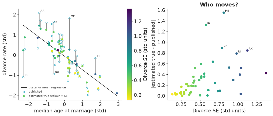
This is shrinkage, the same mechanism as partial pooling in E02. Each state's estimated true rate is a precision-weighted compromise between its published value and what the regression expects for a state like it. Precisely measured states (light colours) do not move. Noisy ones move towards the line, and they move furthest when they are both noisy and far from it - Maine, Idaho, North Dakota. Nobody was deleted, nobody was down-weighted by hand; the likelihood $\text{Normal}(D^\text{true}_i, \text{SE}_i)$ did the weighting.
The same model without the latent variables
Two Normals in a row integrate analytically: $D^\text{obs}_i \sim \text{Normal}\big(\mu_i, \sqrt{\sigma^2 + \text{SE}_i^2}\big)$ - a heteroskedastic likelihood with a known variance component. No latent vector, same posterior for the parameters:
with pm.Model() as marginal_divorce:
    a, bA, bM = pm.Normal("a", 0, 0.2), pm.Normal("bA", 0, 0.5), pm.Normal("bM", 0, 0.5)
    sigma = pm.Exponential("sigma", 1)
    pm.Normal("D_obs", a + bA * A + bM * M_obs, pt.sqrt(sigma**2 + D_se**2), observed=D_obs)
    marginal_divorce_idata = pm.sample(random_seed=RANDOM_SEED, progressbar=False)

coef_table({"latent D_true": errD_idata, "integrated out": marginal_divorce_idata}, var_names=("bA", "bM", "sigma"))
| bA mean | bA std | bM mean | bM std | sigma mean | sigma std | |
|---|---|---|---|---|---|---|
| latent D_true | -0.615 | 0.157 | 0.050 | 0.164 | 0.585 | 0.107 |
| integrated out | -0.617 | 0.157 | 0.048 | 0.165 | 0.587 | 0.106 |
Strip out the predictors and this is random-effects meta-analysis: study estimates $y_j \pm \text{SE}_j$, true effects $\theta_j \sim \text{Normal}(\mu, \tau)$ - the eight-schools model is a measurement-error model. The same two lines handle any input that arrives with an error bar: poll results, small-area statistics, instrument readings, the output of a previous model. (Keep the latent form when you want the $D^\text{true}_i$ themselves, or when the error is in a predictor, where nothing integrates out so neatly.)
8 · Outliers and heavy tails
The third kind of imperfection is the point that does not fit. The reflex is to find it and delete it. The Bayesian workflow has better tools for both halves of that sentence.
Find influential points with PSIS-LOO, not by eye
PSIS-LOO approximates leaving each observation out in turn. Two pointwise by-products: the
Pareto $\hat k$ says how much the posterior would change without that point (above 0.7
the approximation itself fails - the point is highly influential), and elpd_i says how
surprising the point is to a model that has not seen it.
with naive_model:
    pm.compute_log_likelihood(naive_idata, progressbar=False)
naive_loo = az.loo(naive_idata, pointwise=True)

influence = pd.DataFrame({
    "pareto_k": naive_loo.pareto_k.values, "elpd_i": naive_loo.elpd_i.values,
    "Divorce": waffle.Divorce.values, "Divorce SE": waffle["Divorce SE"].values,
    "MedianAgeMarriage": waffle.MedianAgeMarriage.values,
}, index=STATES)
influence.sort_values("pareto_k", ascending=False).head(5).round(2)
| pareto_k | elpd_i | Divorce | Divorce SE | MedianAgeMarriage | |
|---|---|---|---|---|---|
| ID | 0.62 | -6.25 | 7.7 | 1.05 | 23.2 |
| DC | 0.43 | -0.89 | 6.3 | 1.89 | 29.7 |
| ND | 0.30 | -1.94 | 8.0 | 1.44 | 25.3 |
| AR | 0.29 | -2.24 | 13.5 | 1.22 | 24.3 |
| ME | 0.29 | -3.88 | 13.0 | 1.48 | 26.4 |
No $\hat k$ crosses 0.7, so nothing is pathological, but Idaho stands apart on both columns. The two columns measure different things: the District of Columbia has the second-highest $\hat k$ because its age at marriage is extreme (leverage), yet it is well predicted; Maine has an ordinary $\hat k$ but is the second most surprising state. Idaho marries young and divorces little (the usual explanation is its large Latter-day Saints population); Maine divorces far more than its age at marriage suggests. Three responses:
- delete Idaho and refit;
- a Student-t likelihood, which expects an occasional large residual and therefore lets one pull less;
- ask whether the point is an outlier at all, or a noisy measurement - which we do last.
What $\nu$ means
The Student-t has one extra parameter, the degrees of freedom $\nu$. At $\nu = 1$ it is the
Cauchy; below about 5 the tails are heavy enough to shrug off a gross outlier; by
$\nu \approx 30$ it is indistinguishable from a Normal. $\nu$ is a statement about how
often wild residuals occur, so it is informed only by the tails - and 50 data points have
hardly any tail. A sensible default prior is Gamma(2, 0.1) (mean 20, most mass between 3
and 50; Juarez and Steel 2010), which lets the data argue for heavy tails without presuming
them. The alternative is to fix a small $\nu$ as a deliberate robustness assumption, as
McElreath does with $\nu = 2$. Note that sigma of a Student-t is a scale, not a standard
deviation: do not compare it with the Normal's sigma.
student_model, student_idata = fit_divorce(likelihood="student")
_, student2_idata = fit_divorce(likelihood="student", nu=2.0)
_, no_idaho_idata = fit_divorce(keep=STATES != "ID")

robust_fits = {"Normal, all 50 states": naive_idata, "Normal, Idaho deleted": no_idaho_idata,
               "Student-t, nu ~ Gamma(2, 0.1)": student_idata, "Student-t, nu = 2": student2_idata}
for label, idata in robust_fits.items():
    check(idata, label)

nu = az.extract(student_idata, var_names="nu").values
prior_q = stats.gamma(2, scale=10).ppf([0.03, 0.5, 0.97])
print(f"\nposterior of nu: median {np.median(nu):.0f}, 94% interval {np.quantile(nu, [0.03, 0.97]).round(0)}"
      f"   (the Gamma(2, 0.1) prior: median {prior_q[1]:.0f}, 94% interval {prior_q[[0, 2]].round(0)})")
coef_table(robust_fits, var_names=("bA", "bM"))
Normal, all 50 states              divergences  0   max r_hat 1.000   min ess_bulk 2,005
Normal, Idaho deleted              divergences  0   max r_hat 1.002   min ess_bulk 2,044
Student-t, nu ~ Gamma(2, 0.1)      divergences  0   max r_hat 1.002   min ess_bulk 2,558
Student-t, nu = 2                  divergences  0   max r_hat 1.001   min ess_bulk 2,619

posterior of nu: median 17, 94% interval [ 4. 52.]   (the Gamma(2, 0.1) prior: median 17, 94% interval [ 3. 54.])
| bA mean | bA std | bM mean | bM std | |
|---|---|---|---|---|
| Normal, all 50 states | -0.604 | 0.158 | -0.058 | 0.156 |
| Normal, Idaho deleted | -0.751 | 0.146 | -0.082 | 0.140 |
| Student-t, nu ~ Gamma(2, 0.1) | -0.639 | 0.157 | -0.043 | 0.159 |
| Student-t, nu = 2 | -0.696 | 0.150 | 0.046 | 0.199 |
with student_model:
    pm.compute_log_likelihood(student_idata, progressbar=False)
az.compare({"Normal": naive_idata, "Student-t": student_idata}, round_to=1)
| rank | elpd_diff | dse | p_worse | diag_diff | diag_elpd | p | elpd | se | weight | |
|---|---|---|---|---|---|---|---|---|---|---|
| Student-t | 0 | 0.0 | 0.0 | NaN | 4.7 | -63.4 | 6.2 | 1.0 | ||
| Normal | 1 | -0.5 | 0.8 | 0.7 | N < 100 | 4.8 | -63.9 | 6.5 | 0.0 |
- Deleting one state out of 50 moves $\beta_A$ by about one posterior standard deviation. That is what "influential" means.
- The Student-t with a free $\nu$ barely reacts: the posterior of $\nu$ is essentially its prior, because a single moderately unusual state is no evidence of heavy tails. LOO cannot separate the two likelihoods.
- Fixing $\nu = 2$ imposes robustness and moves $\beta_A$ most of the way to the Idaho-deleted answer without choosing whom to delete. It is an assumption, stated in the model, that you can defend or vary - which is exactly what deleting a row is not.
Outlier, or data error?
Robust likelihoods are for observations that are correct but unusual: the process really does produce an Idaho now and then, and the model should not be thrown by it. A data error - a unit mix-up, a typo, a noisy instrument - is a different thing, and the right response is to fix it or to model the error process. We have already done the latter for these data. Look at what the measurement-error model of section 7 made of the two states LOO singled out:
shift = pd.DataFrame({"Divorce SE": waffle["Divorce SE"].values, "published D (std)": D_obs,
                      "estimated true D (std)": D_true, "shift": D_true - D_obs}, index=STATES)
print(f"median Divorce SE over all states: {waffle['Divorce SE'].median():.2f}")
shift.loc[["ID", "ME"]].round(2)
median Divorce SE over all states: 0.80
| Divorce SE | published D (std) | estimated true D (std) | shift | |
|---|---|---|---|---|
| ID | 1.05 | -1.09 | 0.23 | 1.33 |
| ME | 1.48 | 1.82 | 0.27 | -1.55 |
Both "outliers" have above-median standard errors, and the measurement-error model moved both by more than a full standard deviation of the outcome - further than any other state. It did what the Student-t was asked to do, discounting an extreme point, but for a reason we can point to in the data documentation, and only as far as the known SE allows. A generic heavy tail is the fallback for when you know nothing about why a point is off.
9 · Rounding, heaping, censoring, truncation
The remaining imperfections are all the same trick: the likelihood should describe the number that was written down, not the quantity you wish had been recorded.
| What happened to the value | Likelihood contribution | PyMC |
|---|---|---|
| recorded exactly | density $f(y)$ | any distribution |
| only known to exceed / fall below a bound (censored) | $P(Y > c)$ or $P(Y < c)$ | pm.Censored - see E06 |
| rounded or binned (interval-censored) | $F(\text{upper}) - F(\text{lower})$ | pm.CustomDist around pt.round, or pm.Potential |
| rows beyond a bound never enter the dataset (truncated) | $f(y) / P(\text{inside})$ | pm.Truncated |
The field scales at Palmer were read coarsely, and people like round numbers:
grams = raw["Body Mass (g)"].dropna()
print(f"body masses that are multiples of 25 g: {(grams % 25 == 0).mean():.0%}, "
      f"of 50 g: {(grams % 50 == 0).mean():.0%}, of 100 g: {(grams % 100 == 0).mean():.0%}")
body masses that are multiples of 25 g: 100%, of 50 g: 85%, of 100 g: 48%
Every mass is a multiple of 25 g, and multiples of 50 and 100 are over-represented
(heaping). With a residual sd near 300 g a 25-50 g grid is harmless - rounding matters
when the grid is comparable to the spread. To see it matter, pretend the scale had read to
the nearest kilogram, and compare three fits of mass ~ species + sex.
PyMC can derive the likelihood of a rounded variable by itself: wrap pt.round around a
distribution inside pm.CustomDist and the log-probability becomes
$\log\big[F(y + \tfrac12) - F(y - \tfrac12)\big]$.
sp_s, _, male_s = design(sexed)
mass_exact = sexed.mass.to_numpy()
mass_rounded = np.round(mass_exact)
print("rounded masses (kg: birds):", {int(k): int(n) for k, n in zip(*np.unique(mass_rounded, return_counts=True))})


def rounded_normal(mu, sigma, size):
    return pt.round(pm.Normal.dist(mu, sigma, size=size))


def fit_rounding(y, interval):
    with pm.Model(coords={"species": SPECIES}):
        a = pm.Normal("a", 4, 1, dims="species")
        b_male = pm.Normal("b_male", 0, 1)
        sigma = pm.HalfNormal("sigma", 0.5)
        mu = a[sp_s] + b_male * male_s
        if interval:
            pm.CustomDist("mass", mu, sigma, dist=rounded_normal, observed=y)
        else:
            pm.Normal("mass", mu, sigma, observed=y)
        return pm.sample(random_seed=RANDOM_SEED, progressbar=False)


rounding_fits = {"exact masses": fit_rounding(mass_exact, interval=False),
                 "rounded to 1 kg, Normal likelihood": fit_rounding(mass_rounded, interval=False),
                 "rounded to 1 kg, interval likelihood": fit_rounding(mass_rounded, interval=True)}
for label, idata in rounding_fits.items():
    check(idata, label)
coef_table(rounding_fits, var_names=("sigma", "b_male"))
rounded masses (kg: birds): {3: 68, 4: 153, 5: 79, 6: 33}exact masses divergences 0 max r_hat 1.001 min ess_bulk 1,820 rounded to 1 kg, Normal likelihood divergences 0 max r_hat 1.002 min ess_bulk 2,093 rounded to 1 kg, interval likelihood divergences 0 max r_hat 1.002 min ess_bulk 1,886
| sigma mean | sigma std | b_male mean | b_male std | |
|---|---|---|---|---|
| exact masses | 0.318 | 0.012 | 0.667 | 0.035 |
| rounded to 1 kg, Normal likelihood | 0.461 | 0.018 | 0.667 | 0.051 |
| rounded to 1 kg, interval likelihood | 0.347 | 0.022 | 0.677 | 0.048 |
# trust, but verify: the derived log-probability is the Normal mass of the rounding interval
auto = pm.logp(pm.CustomDist.dist(4.2, 0.3, dist=rounded_normal), 4.0).eval()
by_hand = np.log(stats.norm.cdf(4.5, 4.2, 0.3) - stats.norm.cdf(3.5, 4.2, 0.3))
print(f"pm.logp of the rounded Normal at 4: {auto:.5f}    log[F(4.5) - F(3.5)]: {by_hand:.5f}")
pm.logp of the rounded Normal at 4: -0.18449 log[F(4.5) - F(3.5)]: -0.18449
Treating rounded values as exact inflates $\sigma$: the rounding error (variance $h^2/12$ for a grid of width $h$ - Sheppard's correction) is mistaken for biological variation. The interval likelihood gives most of it back, with a wider posterior because a 1 kg grid really does destroy information. Location parameters are barely affected, which is why rounding is usually ignored - until the question is about a variance, a tail probability or a threshold.
10 · The decision table
| Data problem | What deleting / ignoring assumes | Model-based alternative | PyMC construct |
|---|---|---|---|
| Missing outcome | nothing harmful under MAR (no information lost) | impute only if you need predictions for those rows | observed= with NaN -> y_unobserved, y_observed, y |
| Missing continuous covariate | complete cases are a random subsample (MCAR), or at least missingness is unrelated to the outcome | a distribution for the covariate, conditioned on what predicts it and its missingness | the same NaN idiom on the covariate; use the stitched variable downstream |
| Mean / median fill | the value is known exactly and equals the mean | as above | as above |
| Missing discrete covariate | as for continuous | mixture over its values; posterior class probabilities by Bayes' rule | pm.math.logsumexp + pm.Potential, or pymc_extras.marginalize + recover |
| Value missing because of its value (MNAR) | MAR | selection model: likelihood for the missingness indicator given the latent value; then a sensitivity analysis | pm.Bernoulli("is_missing", logit_p=c0 + c1 * x_completed, observed=...) |
| Outcome measured with known error | measured exactly; equal precision everywhere | latent true value, or add the known variance | pm.Normal("obs", true, se, observed=...) or sigma=pt.sqrt(sigma**2 + se**2) |
| Predictor measured with error | measured exactly (slope attenuated) | latent true predictor with its own model | latent pm.Normal + pm.Normal("x_obs", x_true, se, observed=...) |
| Outlier (correct but unusual) | that point comes from a process you need not describe | heavy-tailed likelihood; find candidates with Pareto $\hat k$ | pm.StudentT, az.loo(pointwise=True) |
| Data error | - | fix at the source, or model the error process (mixture of good and bad readings) | pm.Mixture; known SEs as above |
| Rounded / heaped / binned | the grid is fine relative to the spread | interval likelihood | pm.CustomDist around pt.round; pm.Potential with logdiffexp of pm.logcdf |
| Censored | censored rows are events, or are ignorable (E06: badly wrong) | survival-function contribution | pm.Censored |
| Truncated sample | the sample represents the population | renormalised density | pm.Truncated |
Try it yourself
- Fool the selection model. Its identification leans on Normality. Delete 40% of the
isotope values completely at random and fit the selection model: does the interval of
c1include zero, as it should? Now do the same after replacing $\delta^{15}$N by a right-skewed version of itself (saynp.expof the standardised values) while keeping the Normal covariate model. What does the model make of skewness it did not expect? Finally, in the original experiment, put a sceptical prior onc1(Normal(0, 0.5)): how far do the species means move back towards the MAR answer? - Make mean-filling flip a sign. In the deletion experiment of section 4, let the
mechanism depend on mass standardised over all birds instead of within species and sex,
with slope 3 and intercept 0, so that the small species lose nearly all their isotope
values. Compare the least-squares estimates over 200 deletions (
ols_b_nis fast), then fit the joint model to a handful of them. Why is mean-filling now worse than useless? - Give the unsexed birds a better classifier. Add bill depth to the hand-written mixture of section 5 with a species- and sex-specific mean. Which of the nine posterior probabilities change, and does $\beta_N$ care?
Next: D03 for exploratory analysis and reporting, or E06 for censoring in depth.