In E01-E06 the regression function was something we chose: a line, a spline, a GP. Here we do not get to choose. General relativity plus a list of what the universe contains predicts, with no free functional form, how bright a standard candle looks at redshift $z$. The theory is the regression function. That changes the character of every step:
- parameters have units and meaning (the fraction of the universe that is matter), so priors come from physics rather than from "weakly informative" folklore;
- extrapolation is principled - the curve beyond the data is a prediction of the theory, not the whim of a basis function;
- model comparison answers a scientific question. "Does the model with a cosmological constant predict better than the one without?" is the question that won the 2011 Nobel prize in physics: is the expansion of the universe accelerating?
The price is computational: the theory contains an integral with no closed form, and it has to live inside the model, differentiable, for 580 supernovae at once.
import arviz as az
import matplotlib.pyplot as plt
import numpy as np
import pandas as pd
import pymc as pm
import pytensor
import pytensor.tensor as pt
from scipy import integrate, stats

from pymc_challenges import data

RANDOM_SEED = 1998
rng = np.random.default_rng(RANDOM_SEED)
az.style.use("arviz-variat")

print(f"PyMC {pm.__version__}, ArviZ {az.__version__}, PyTensor {pytensor.__version__}")
PyMC 6.3.2, ArviZ 1.3.0, PyTensor 3.3.2
1 · Question and data
A type Ia supernova is a white dwarf that explodes at (very nearly) a fixed mass, so its peak luminosity is (very nearly) the same everywhere: a standard candle. Compare how bright it is (absolute magnitude $M$) with how bright it looks (apparent magnitude $m$) and you have its distance, reported as the distance modulus
$$\mu = m - M = 5\log_{10}\!\frac{d_L}{10\ \text{pc}}$$
where $d_L$ is the luminosity distance. Five magnitudes are a factor 100 in flux, so $\Delta\mu = 0.1$ is about 5% in distance. The redshift $z$ of the host galaxy says how much the universe has expanded since the light left. Distance against redshift - the Hubble diagram - is therefore a record of the expansion history.
data.describe("supernovae")
sn = data.load("supernovae").sort_values("z").reset_index(drop=True)
z_obs, mu_obs, mu_err = sn.z.values, sn.mu.values, sn.mu_err.values
sn.describe().round(3)
supernovae: 580 type Ia supernovae: redshift z, distance modulus mu and its error.
  source: Supernova Cosmology Project, Union2.1 compilation (Suzuki et al. 2012).
  url:    https://supernova.lbl.gov/Union/figures/SCPUnion2.1_mu_vs_z.txt
| z | mu | mu_err | p_low_mass_host | |
|---|---|---|---|---|
| count | 580.000 | 580.000 | 580.000 | 580.000 |
| mean | 0.362 | 40.028 | 0.223 | 0.424 |
| std | 0.327 | 3.196 | 0.126 | 0.277 |
| min | 0.015 | 33.825 | 0.084 | 0.000 |
| 25% | 0.055 | 36.920 | 0.151 | 0.128 |
| 50% | 0.294 | 40.884 | 0.189 | 0.552 |
| 75% | 0.552 | 42.518 | 0.242 | 0.552 |
| max | 1.414 | 45.411 | 1.007 | 1.000 |
fig, ax = plt.subplots(figsize=(8, 4.5))
ax.errorbar(z_obs, mu_obs, yerr=mu_err, fmt=".", ms=3, lw=0.5, color="k", alpha=0.5)
ax.set(xscale="log", xlabel="redshift z", ylabel=r"distance modulus $\mu$ (mag)",
       title="Union2.1 Hubble diagram: 580 type Ia supernovae");
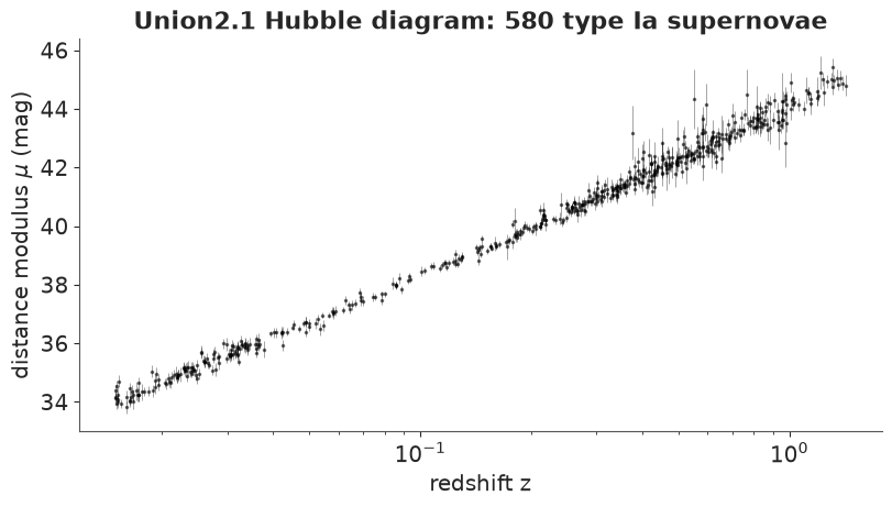
Nearly twelve magnitudes of dynamic range and a curve that looks like a boring logarithm. Almost all of that is just "further away is fainter". Everything interesting - the entire evidence for dark energy - is a deviation of a few tenths of a magnitude at $z > 0.3$, comparable to the error bar of a single supernova. We will need a better way to look at it (section 5) and a model that uses all 580 objects at once.
2 · The physics, compactly
In a homogeneous, isotropic universe the expansion rate is $H(z) = H_0\,E(z)$, where the Friedmann equation gives the dimensionless function
$$E(z)^2 = \Omega_m (1+z)^3 + \Omega_k (1+z)^2 + \Omega_{\Lambda}\,(1+z)^{3(1+w)}, \qquad \Omega_k = 1 - \Omega_m - \Omega_\Lambda .$$
$\Omega_m$ is today's matter density and $\Omega_\Lambda$ the dark-energy density, both as fractions of the critical density; $\Omega_k$ is whatever is left over and shows up as spatial curvature. $w$ is the dark-energy equation of state (pressure / energy density): $w=-1$ is Einstein's cosmological constant, whose density does not dilute as space expands.
Light travelling towards us covers the dimensionless comoving distance
$$\chi(z) = \int_0^z \frac{dz'}{E(z')}$$
and the luminosity distance is
$$d_L(z) = (1+z)\,\frac{c}{H_0}\;\text{sinn}(\chi;\Omega_k), \qquad \text{sinn}(\chi;\Omega_k) = \begin{cases} \sinh(\sqrt{\Omega_k}\,\chi)/\sqrt{\Omega_k} & \Omega_k > 0 \ \text{(open)}\\ \chi & \Omega_k = 0 \ \text{(flat)}\\ \sin(\sqrt{-\Omega_k}\,\chi)/\sqrt{-\Omega_k} & \Omega_k < 0 \ \text{(closed)} \end{cases}$$
With $c$ in km/s and $H_0$ in km/s/Mpc, $c/H_0$ is in Mpc, and 1 Mpc = $10^5 \times$ 10 pc, so
$$\mu(z) = \underbrace{5\log_{10}\big[(1+z)\,\text{sinn}(\chi)\big]}_{\text{shape: depends on }\Omega_m,\,\Omega_\Lambda,\,w} \;+\; \underbrace{25 + 5\log_{10}\frac{c}{H_0\,[\text{Mpc}]}}_{\text{a constant}} .$$
Every model in this notebook is a constraint on the same function:
| model | $\Omega_m$ | $\Omega_\Lambda$ | $w$ | story |
|---|---|---|---|---|
| (a) Einstein-de Sitter | 1 | 0 | - | matter only; the textbook universe before 1998 |
| (b) flat $\Lambda$CDM | free | $1-\Omega_m$ | $-1$ | today's standard model |
| (c) curved $\Lambda$CDM | free | free | $-1$ | let the data decide on flatness |
| (d) flat $w$CDM | free | $1-\Omega_m$ | free | is dark energy really a constant? |
The quantity that answers the headline question is the deceleration parameter today, $q_0 = -\ddot a a/\dot a^2 = \tfrac12\Omega_m + \tfrac12(1+3w)\,\Omega_\Lambda$, which for $w=-1$ is $\Omega_m/2 - \Omega_\Lambda$. Matter pulls the brake; $q_0 < 0$ means the expansion is speeding up.
3 · The computational core: an integral inside the model
$\chi(z)$ has no closed form for general $(\Omega_m, \Omega_\Lambda, w)$. NUTS needs the
log-density and its gradient with respect to the parameters, so
scipy.integrate.quad is out: PyTensor cannot differentiate through it. Options:
- Fixed-order Gauss-Legendre quadrature per supernova. Map the $K$ nodes $x_k$ and weights $w_k$ from $[-1, 1]$ onto $[0, z_i]$: $\chi(z_i) \approx \frac{z_i}{2}\sum_k w_k \,/\, E\!\big(\tfrac{z_i}{2}(x_k+1)\big)$. That is a $(580 \times K)$ array of plain arithmetic - trivially vectorised, and differentiable because it is just arithmetic. $1/E$ is very smooth, so a small $K$ gives machine precision.
- A cumulative trapezoid/Simpson rule on a fine shared $z$-grid, then interpolate to each $z_i$. Fine too, but the accuracy depends on grid and interpolation.
- Write the integral in JAX and bring it in with
pytensor.wrap_jax(the subject of E09). The right tool when the numerics need adaptive control flow; overkill here.
We take option 1. The functions below only use arithmetic, sqrt, log10 and maximum,
so the same code runs on NumPy arrays (for checking and for posterior curves) and on
PyTensor variables (inside the model) - pass xp=np or xp=pt, as C01 did.
One subtlety: $\text{sinn}$. The obvious pt.switch between sinh, sin and $\chi$
returns the right value everywhere, but its gradient at $\Omega_k = 0$ - exactly where
flat models live - is NaN: the derivative of $\sqrt{|\Omega_k|}$ in the unused branches is
infinite there and leaks through the switch. But $\text{sinn}$ is an entire function of
$\Omega_k$: both branches are the same power series
$\chi\,\sum_n (\Omega_k\chi^2)^n/(2n+1)!$. For $|\Omega_k\chi^2| \lesssim 2$, which covers
anything remotely relevant, nine terms are exact to double precision. No branches, no NaN.
C_KMS = 299_792.458  # speed of light, km/s
H0_FID = 70.0  # km/s/Mpc - the value the published mu assume (section 4)
MU0_FID = 25 + 5 * np.log10(C_KMS / H0_FID)  # the constant in mu(z) for h = 0.7


def _nodes_axis(p):
    """Give array-valued parameters a trailing axis so they broadcast against quadrature nodes."""
    return p[..., None] if getattr(p, "ndim", 0) > 0 else p


def E2(z, Om, OL, w=-1.0):
    """Friedmann equation: (H(z) / H0)^2 for matter + curvature + dark energy."""
    Ok = 1 - Om - OL
    return Om * (1 + z) ** 3 + Ok * (1 + z) ** 2 + OL * (1 + z) ** (3 * (1 + w))


def comoving_distance(z, Om, OL, w=-1.0, xp=np, n_nodes=16):
    """chi(z) = int_0^z dz'/E(z') by Gauss-Legendre quadrature; z has shape (..., N)."""
    x_k, w_k = np.polynomial.legendre.leggauss(n_nodes)
    nodes = 0.5 * z[..., None] * (x_k + 1)  # (..., N, K) points inside [0, z_i]
    e2 = E2(nodes, _nodes_axis(Om), _nodes_axis(OL), _nodes_axis(w))
    e2 = xp.maximum(e2, 1e-8)  # E^2 <= 0 means "no Big Bang": see model (c)
    return 0.5 * z * (w_k / xp.sqrt(e2)).sum(-1)


def sinn(chi, Ok, n_terms=9):
    """sinh(sqrt(Ok) chi)/sqrt(Ok), chi, or sin(sqrt(-Ok) chi)/sqrt(-Ok) - as one power series."""
    u = Ok * chi**2
    term, total = 1.0, 1.0
    for n in range(1, n_terms):
        term = term * u / ((2 * n) * (2 * n + 1))
        total = total + term
    return chi * total


def mu_shape(z, Om, OL, w=-1.0, xp=np, n_nodes=16):
    """5 log10 of the dimensionless luminosity distance (H0/c) d_L. Add MU0_FID for h = 0.7."""
    chi = comoving_distance(z, Om, OL, w, xp=xp, n_nodes=n_nodes)
    return 5 * xp.log10((1 + z) * sinn(chi, 1 - Om - OL))
Verify before you trust
A numerical approximation inside a likelihood is a silent source of bias, so we test it three ways before it goes anywhere near a sampler.
Units. A standard benchmark: for $\Omega_m = 0.3$, flat, $h = 0.7$, the distance modulus at $z = 0.5$ is 42.26. And the empty ("Milne") universe has the closed form $(H_0/c)\,d_L = z(1 + z/2)$, which exercises the $\sinh$ branch of the series.
print(f"mu(z=0.5 | Om=0.3, flat, h=0.7) = {float(mu_shape(np.array([0.5]), 0.3, 0.7)[0] + MU0_FID):.3f}")

z_test = np.array([0.01, 0.1, 0.5, 1.0, 1.414, 3.0])
milne_exact = 5 * np.log10(z_test * (1 + z_test / 2))
print("empty universe, max |error| vs closed form:", np.abs(mu_shape(z_test, 0.0, 0.0) - milne_exact).max())
mu(z=0.5 | Om=0.3, flat, h=0.7) = 42.261
empty universe, max |error| vs closed form: 7.993605777301127e-15
Accuracy against adaptive quadrature, at every observed redshift, for cosmologies spread over (and beyond) the region the sampler will explore - including strongly open, closed and phantom ($w < -1$) cases - as a function of the number of nodes:
def mu_shape_quad(z, Om, OL, w=-1.0):
    """Reference implementation: scipy.integrate.quad and explicit sin/sinh branches."""
    chi = integrate.quad(lambda x: 1 / np.sqrt(E2(x, Om, OL, w)), 0, z, epsabs=1e-13, epsrel=1e-13)[0]
    Ok = 1 - Om - OL
    if Ok > 1e-12:
        chi = np.sinh(np.sqrt(Ok) * chi) / np.sqrt(Ok)
    elif Ok < -1e-12:
        chi = np.sin(np.sqrt(-Ok) * chi) / np.sqrt(-Ok)
    return 5 * np.log10((1 + z) * chi)


test_cosmologies = {
    "Einstein-de Sitter (1, 0)": (1.0, 0.0, -1.0),
    "flat LCDM (0.3, 0.7)": (0.3, 0.7, -1.0),
    "open (0.2, 0)": (0.2, 0.0, -1.0),
    "closed (0.8, 1.2)": (0.8, 1.2, -1.0),
    "phantom w=-2 (0.3, 0.7)": (0.3, 0.7, -2.0),
    "w=-0.5 (0.1, 0.9)": (0.1, 0.9, -0.5),
}
accuracy = {}
for label, pars in test_cosmologies.items():
    exact = np.array([mu_shape_quad(zi, *pars) for zi in z_obs])
    accuracy[label] = {K: np.abs(mu_shape(z_obs, *pars, n_nodes=K) - exact).max() for K in (2, 4, 8, 16)}

pd.DataFrame(accuracy).T.rename_axis("max |error| in mag, by number of nodes", axis=1).map("{:.1e}".format)
| max |error| in mag, by number of nodes | 2 | 4 | 8 | 16 |
|---|---|---|---|---|
| Einstein-de Sitter (1, 0) | 1.6e-02 | 5.1e-05 | 3.5e-10 | 1.8e-15 |
| flat LCDM (0.3, 0.7) | 3.6e-03 | 7.7e-06 | 2.3e-11 | 1.8e-15 |
| open (0.2, 0) | 9.2e-03 | 2.1e-05 | 1.1e-10 | 2.7e-15 |
| closed (0.8, 1.2) | 9.9e-03 | 3.9e-05 | 7.1e-09 | 1.8e-15 |
| phantom w=-2 (0.3, 0.7) | 3.4e-02 | 5.4e-04 | 1.7e-07 | 9.8e-15 |
| w=-0.5 (0.1, 0.9) | 4.2e-03 | 8.2e-06 | 3.5e-11 | 1.8e-15 |
The smallest measurement error in the data is 0.08 mag. Four nodes would already be more than good enough; with 16 the quadrature error is at the level of floating-point rounding ($10^{-14}$ mag) for every test case, exotic ones included. We keep 16: a $580 \times 16$ array costs nothing.
Gradient. Finally, check that PyTensor differentiates through the whole thing, by comparing $\partial\mu/\partial\Omega_m$ with a finite difference.
Om_, OL_, w_ = pt.dscalars("Om", "OL", "w")
mu_graph = mu_shape(z_test, Om_, OL_, w_, xp=pt)
dmu_dOm = pytensor.function([Om_, OL_, w_], pytensor.gradient.jacobian(mu_graph, Om_))

eps = 1e-6
finite_diff = (mu_shape(z_test, 0.3 + eps, 0.7) - mu_shape(z_test, 0.3 - eps, 0.7)) / (2 * eps)
pd.DataFrame({"z": z_test, "autodiff": dmu_dOm(0.3, 0.7, -1.0), "finite difference": finite_diff}).round(6)
| z | autodiff | finite difference | |
|---|---|---|---|
| 0 | 0.010 | -0.005500 | -0.005500 |
| 1 | 0.100 | -0.061000 | -0.061000 |
| 2 | 0.500 | -0.392660 | -0.392660 |
| 3 | 1.000 | -0.851740 | -0.851740 |
| 4 | 1.414 | -1.193284 | -1.193284 |
| 5 | 3.000 | -2.116422 | -2.116422 |
Note the size of the signal: at $z = 1$, changing $\Omega_m$ by 0.1 (at fixed $\Omega_\Lambda$) moves $\mu$ by less than a tenth of a magnitude, while a single supernova is measured to about 0.2 mag. This is a many-objects, small-effect problem - exactly where a joint probabilistic model earns its keep.
4 · Something goes wrong: $H_0$ and $M$
Let us write the "obvious" flat $\Lambda$CDM model. The theory has two parameters, $\Omega_m$ and $H_0$, so give both a prior: $\Omega_m \sim \text{Uniform}(0,1)$ and $H_0 \sim \text{Uniform}(40, 100)$ km/s/Mpc, which brackets every measurement of the last fifty years. And a standard candle is only useful if you know its wattage: the published $\mu$ were computed with an assumed absolute magnitude $M$, which could be off, so add $\delta M \sim \text{Normal}(0, 1)$ for the calibration error. Finally, supernovae are not perfectly standard: add an intrinsic scatter $\sigma_\text{int}$ in quadrature to the quoted errors, with a prior that knows type Ia scatter is of order 0.1 mag.
$$\mu_i^\text{obs} \sim \text{Normal}\Big(\mu_\text{shape}(z_i;\Omega_m) + 25 + 5\log_{10}\tfrac{c}{H_0} + \delta M,\ \ \sqrt{\sigma_i^2 + \sigma_\text{int}^2}\Big)$$
coords = {"sn": sn.name.values}

with pm.Model(coords=coords) as naive_model:
    Om = pm.Uniform("Om", 0.0, 1.0)
    H0 = pm.Uniform("H0", 40.0, 100.0)  # floats! see the note below
    dM = pm.Normal("dM", 0.0, 1.0)
    sigma_int = pm.HalfNormal("sigma_int", 0.2)

    mu = mu_shape(z_obs, Om, 1 - Om, xp=pt) + 25 + 5 * pt.log10(C_KMS / H0) + dM
    pm.Normal("mu_obs", mu, pt.sqrt(mu_err**2 + sigma_int**2), observed=mu_obs, dims="sn")

    naive_idata = pm.sample(random_seed=RANDOM_SEED)

print("divergences:", int(naive_idata.sample_stats["diverging"].sum()))
az.summary(naive_idata, round_to=3)
divergences: 4
| mean | sd | eti89_lb | eti89_ub | ess_bulk | ess_tail | r_hat | mcse_mean | mcse_sd | |
|---|---|---|---|---|---|---|---|---|---|
| dM | 0.065 | 0.523 | -0.955 | 0.683 | 46.266 | 237.059 | 1.091 | 0.085 | 0.022 |
| Om | 0.279 | 0.020 | 0.249 | 0.312 | 457.031 | 268.529 | 1.010 | 0.001 | 0.000 |
| H0 | 74.081 | 16.214 | 45.027 | 95.789 | 46.380 | 234.363 | 1.091 | 2.748 | 0.583 |
| sigma_int | 0.017 | 0.012 | 0.001 | 0.040 | 660.080 | 605.361 | 1.004 | 0.000 | 0.000 |
(A PyMC trap met on the way: pm.Uniform("H0", 40, 100) with integer bounds gives a
NaN initial point and nutpie dies with "All initialization points failed" - small
integer constants become int8, and $40 + 100$ overflows where the interval transform
computes its starting point. Uniform(0, 1) is unaffected. Write bounds as floats.)
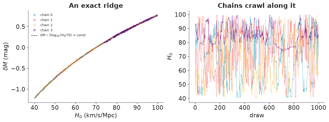
H0 and dM are in trouble: r_hat of 1.09 and an effective sample size below 50 out of
4000 draws, plus a few divergences. Even Om, which the data constrain well, mixes worse
than it should. The pair plot shows why.
naive_post = naive_idata.posterior
h_line = np.linspace(40, 100, 200)
ridge_const = float((naive_post["dM"] - 5 * np.log10(naive_post["H0"] / H0_FID)).mean())

fig, axes = plt.subplots(1, 2, figsize=(11, 4))
for chain in naive_post.chain.values:
    axes[0].plot(naive_post["H0"].sel(chain=chain), naive_post["dM"].sel(chain=chain), ".", ms=2,
                 alpha=0.4, label=f"chain {chain}")
axes[0].plot(h_line, ridge_const + 5 * np.log10(h_line / H0_FID), "k--", lw=1,
             label=r"$\delta M - 5\log_{10}(H_0/70)$ = const")
axes[0].set(xlabel=r"$H_0$ (km/s/Mpc)", ylabel=r"$\delta M$ (mag)", title="An exact ridge")
axes[0].legend(markerscale=5, fontsize=8)
axes[1].plot(naive_post["H0"].values.T, lw=0.5)
axes[1].set(xlabel="draw", ylabel=r"$H_0$", title="Chains crawl along it");
combo = naive_post["dM"] - 5 * np.log10(naive_post["H0"] / H0_FID)
print(f"posterior sd of H0          : {float(naive_post['H0'].std()):.1f}   (prior sd of Uniform(40, 100): {60 / np.sqrt(12):.1f})")
print(f"posterior sd of dM          : {float(naive_post['dM'].std()):.2f}")
print(f"posterior sd of the combo   : {float(combo.std()):.3f}")
posterior sd of H0          : 16.2   (prior sd of Uniform(40, 100): 17.3)
posterior sd of dM          : 0.52
posterior sd of the combo   : 0.011
Every draw sits on the curve $\delta M - 5\log_{10}H_0 = \text{const}$. Look back at the
likelihood: $H_0$ and $\delta M$ enter only through that sum. A universe that expands
10% faster with supernovae that are 0.2 mag fainter produces exactly the same data. No
amount of supernovae can separate them; the data pin the combination to about a hundredth
of a magnitude, and along the ridge the posterior is simply the prior (the posterior sd of
$H_0$ is nearly that of Uniform(40, 100); the $\delta M$ prior trims the ends a little). A
ridge fifty times longer than it is wide, curved, with hard walls at both ends, is
miserable for a sampler with a diagonal mass matrix - hence the diagnostics.
The tempting reaction is to turn sampler knobs:
with naive_model:
    naive_idata_095 = pm.sample(target_accept=0.95, random_seed=RANDOM_SEED)

print("divergences:", int(naive_idata_095.sample_stats["diverging"].sum()))
print(f"posterior sd of H0: {float(naive_idata_095.posterior['H0'].std()):.1f}")
az.summary(naive_idata_095, var_names=["H0", "dM"], round_to=3)
divergences: 0
posterior sd of H0: 15.7
| mean | sd | eti89_lb | eti89_ub | ess_bulk | ess_tail | r_hat | mcse_mean | mcse_sd | |
|---|---|---|---|---|---|---|---|---|---|
| H0 | 70.292 | 15.745 | 45.868 | 95.225 | 385.163 | 461.452 | 1.012 | 0.790 | 0.339 |
| dM | -0.048 | 0.508 | -0.913 | 0.669 | 385.334 | 461.663 | 1.012 | 0.026 | 0.013 |
The diagnostics now look almost respectable, and nothing has been learned: the "posterior" of $H_0$ is still the prior. This is the dangerous version of the problem - more careful sampling hides the symptom, and a reader of the summary table would happily report $H_0 \approx 70 \pm 16$ "from supernovae". It is not a sampler problem. The model asks the data a question they cannot answer.
(This is why measuring $H_0$ needs a distance ladder: Cepheids or some other rung to calibrate $M$ independently. It is also why the tension between different $H_0$ measurements does not touch the evidence for acceleration, which lives in the shape.)
The fix is to model what is identified. Collapse the two into one nuisance parameter:
$$\text{offset} = \delta M - 5\log_{10}(h/0.7)$$
The Union2.1 distance moduli are published for a fiducial calibration equivalent to
$h = H_0/100 = 0.7$, so we write $\mu = \mu_\text{shape} + \mu_0(h{=}0.7) + \text{offset}$
and expect an offset near zero. Its prior can come from physics: $h$ between 0.5 and 1 is
$\pm 0.75$ mag, so Normal(0, 0.5) is honest. Because the offset enters linearly with
Gaussian noise it could even be integrated out analytically, as many published analyses
do; we sample it instead, so that the pointwise log-likelihood needed for LOO stays simple.
Every model below shares the same nuisance parameters and likelihood, so wrap them once:
def hubble_likelihood(shape, student_t=False):
    """Shared part of every model: identified offset, intrinsic scatter, likelihood."""
    offset = pm.Normal("offset", 0.0, 0.5)
    sigma_int = pm.HalfNormal("sigma_int", 0.2)
    mu = pm.Deterministic("mu", shape + MU0_FID + offset, dims="sn")
    sigma = pt.sqrt(mu_err**2 + sigma_int**2)
    if student_t:
        nu = pm.Gamma("nu", 2.0, 0.1)
        pm.StudentT("mu_obs", nu=nu, mu=mu, sigma=sigma, observed=mu_obs, dims="sn")
    else:
        pm.Normal("mu_obs", mu, sigma, observed=mu_obs, dims="sn")


with pm.Model(coords=coords) as flat_model:
    Om = pm.Uniform("Om", 0.0, 1.0)
    pm.Deterministic("OL", 1 - Om)
    hubble_likelihood(mu_shape(z_obs, Om, 1 - Om, xp=pt))

flat_model
5 · Prior predictive check, in the Hubble diagram
$\Omega_m \sim \text{Uniform}(0, 1)$ is the physical range for a flat universe with non-negative matter and dark-energy densities. What does the prior claim about data?
The raw Hubble diagram hides everything (section 1), so cosmologists plot residuals against a reference: the empty universe ($\Omega_m = \Omega_\Lambda = 0$), which neither accelerates nor decelerates. Points above zero are fainter - further away - than coasting would predict: the expansion has sped up since the light left. Below zero: slowed down.
with flat_model:
    flat_idata = pm.sample_prior_predictive(500, var_names=["Om", "offset", "sigma_int", "mu_obs"],
                                            random_seed=RANDOM_SEED)


def milne(z):
    """Distance modulus of the empty universe for h = 0.7 - the reference for residual plots."""
    return 5 * np.log10(z * (1 + z / 2)) + MU0_FID


Z_EDGES = np.array([0.01, 0.03, 0.05, 0.1, 0.2, 0.3, 0.4, 0.5, 0.6, 0.8, 1.0, 1.45])
bin_idx = np.digitize(z_obs, Z_EDGES) - 1
n_bins = len(Z_EDGES) - 1
weights = 1 / mu_err**2


def binned_mean(values):
    """Inverse-variance weighted mean per redshift bin; values has shape (..., 580)."""
    return np.stack([(values[..., bin_idx == b] * weights[bin_idx == b]).sum(-1) / weights[bin_idx == b].sum()
                     for b in range(n_bins)], axis=-1)


z_bin = binned_mean(z_obs)
resid_bin = binned_mean(mu_obs - milne(z_obs))
resid_bin_se = np.array([weights[bin_idx == b].sum() ** -0.5 for b in range(n_bins)])

z_grid = np.geomspace(0.01, 2.5, 200)
prior = az.extract(flat_idata, group="prior", num_samples=100, random_seed=RANDOM_SEED)
Om_prior, offset_prior = prior["Om"].values[:, None], prior["offset"].values[:, None]
prior_curves = mu_shape(z_grid, Om_prior, 1 - Om_prior) + MU0_FID + offset_prior

fig, axes = plt.subplots(1, 2, figsize=(12, 4.2))
axes[0].plot(z_grid, prior_curves.T, color="C0", alpha=0.15, lw=1)
axes[0].errorbar(z_obs, mu_obs, yerr=mu_err, fmt=".", ms=2, lw=0.4, color="k", alpha=0.4)
axes[0].set(xscale="log", xlabel="z", ylabel=r"$\mu$", title="Prior curves, Hubble diagram")
sm = plt.cm.ScalarMappable(cmap="viridis", norm=plt.Normalize(0, 1))
for om, curve in zip(Om_prior.ravel(), (prior_curves - offset_prior - milne(z_grid))):
    axes[1].plot(z_grid, curve, color=sm.to_rgba(om), alpha=0.5, lw=1)
axes[1].errorbar(z_bin, resid_bin, yerr=resid_bin_se, fmt="o", ms=4, color="k", label="data, binned")
axes[1].axhline(0, color="k", lw=1)
axes[1].axvline(z_obs.max(), color="k", ls=":", lw=1)
axes[1].set(xlabel="z", ylabel=r"$\mu - \mu_\mathrm{empty}$ (mag)",
            title="Same curves, offset removed, vs empty universe")
axes[1].legend()
fig.colorbar(sm, ax=axes[1], label=r"$\Omega_m$");
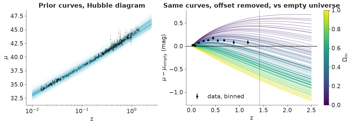
Left: the prior is a band about $\pm 1$ mag wide around the data - that is the offset prior, i.e. our ignorance of $h$ and $M$ - and the shape differences are invisible. Right: the same 100 curves with the offset removed. Now the prior's actual content is clear: it spans everything from a matter-only universe (yellow, always decelerating, $-0.5$ mag at $z = 1$) to pure dark energy (purple). All of them agree at $z \to 0$, where every cosmology reduces to Hubble's law, and fan out with redshift. The binned data (taking the published calibration at face value) already hint where this is going, and the dotted line marks the end of the data: everything right of it is extrapolation by the theory.
The helper binned_mean and the 11 redshift bins will come back for the posterior
predictive checks.
6 · The model ladder
(a) Einstein-de Sitter: matter only
Until the mid-1990s the theoretically favoured universe was flat and made of matter: $\Omega_m = 1$. No cosmological parameter is free - only the two nuisance parameters.
From here on we sample with target_accept=0.95, for a stated reason: in the good models
$\sigma_\text{int}$ turns out to be squeezed against zero, and at the default 0.8 nutpie
typically reports a few divergences down there. Each model samples in a second or two, so
the smaller step size is free.
SAMPLE_KWARGS = dict(target_accept=0.95, random_seed=RANDOM_SEED)

with pm.Model(coords=coords) as eds_model:
    hubble_likelihood(mu_shape(z_obs, 1.0, 0.0, xp=pt))
    eds_idata = pm.sample(**SAMPLE_KWARGS)

print("divergences:", int(eds_idata.sample_stats["diverging"].sum()))
az.summary(eds_idata, var_names=["offset", "sigma_int"], round_to=3)
divergences: 0
| mean | sd | eti89_lb | eti89_ub | ess_bulk | ess_tail | r_hat | mcse_mean | mcse_sd | |
|---|---|---|---|---|---|---|---|---|---|
| offset | 0.249 | 0.011 | 0.231 | 0.266 | 2386.332 | 2394.747 | 1.001 | 0.0 | 0.0 |
| sigma_int | 0.175 | 0.011 | 0.157 | 0.194 | 2382.135 | 2339.287 | 1.002 | 0.0 | 0.0 |
The sampler is perfectly happy - two well-identified parameters. Clean diagnostics say nothing about whether the model is right. Two numbers are suspicious, though: an offset of a quarter of a magnitude (taken at face value, $h \approx 0.62$), and an intrinsic scatter as large as a typical measurement error. Hold that thought until we have something to compare with.
(b) Flat $\Lambda \text{CDM}$
with flat_model:
    flat_idata.update(pm.sample(**SAMPLE_KWARGS))

print("divergences:", int(flat_idata.sample_stats["diverging"].sum()))
az.summary(flat_idata, var_names=["Om", "OL", "offset", "sigma_int"], round_to=3)
divergences: 0
| mean | sd | eti89_lb | eti89_ub | ess_bulk | ess_tail | r_hat | mcse_mean | mcse_sd | |
|---|---|---|---|---|---|---|---|---|---|
| Om | 0.279 | 0.020 | 0.248 | 0.310 | 1231.956 | 1666.015 | 1.002 | 0.001 | 0.0 |
| OL | 0.721 | 0.020 | 0.690 | 0.752 | 1231.956 | 1666.015 | 1.002 | 0.001 | 0.0 |
| offset | 0.001 | 0.011 | -0.016 | 0.018 | 1314.755 | 1750.297 | 1.002 | 0.000 | 0.0 |
| sigma_int | 0.018 | 0.013 | 0.002 | 0.041 | 1288.638 | 959.148 | 1.001 | 0.000 | 0.0 |
az.plot_trace_dist(flat_idata, var_names=["Om", "offset", "sigma_int"]);
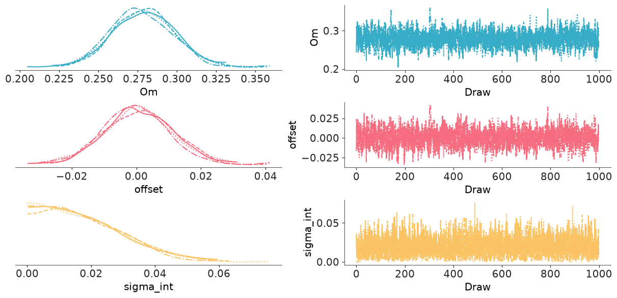
No divergences, r_hat at 1.00, four chains on top of each other, and the offset is now
pinned to about $\pm 0.01$ mag. The effective sample size is "only" a third of the draws
because $\Omega_m$ and the offset are correlated at about 0.7 (a lower $\Omega_m$ makes
distant supernovae fainter; so does a higher offset) - plenty for our purposes. One
consequence worth knowing: az.plot_rank, which E01 recommended, draws its envelope for
independent draws, so with this much autocorrelation it tends to flag perfectly healthy
chains. Thin the draws before using it, or rely on r_hat and ESS, which account for
autocorrelation.
The physics:
- $\Omega_m \approx 0.28$: matter is only about 28% of the critical density, and if the universe is flat the other 72% is something that behaves like a cosmological constant.
- The offset is consistent with zero: the published $\mu$ indeed correspond to $h = 0.7$.
- $\sigma_\text{int}$ is consistent with zero, while Einstein-de Sitter needed 0.17 mag. Two lessons in one. First, the published errors evidently already contain an intrinsic-dispersion term (compilations like this one tune it so that the best fit has $\chi^2$ per degree of freedom near one - computed below), leaving nothing for ours to do. Second, a free scatter term is a misfit sponge: in model (a) it quietly soaked up the failure of the physics. A large "noise" estimate is a symptom worth chasing.
flat_post = az.extract(flat_idata)
mu_hat = mu_shape(z_obs, float(flat_post["Om"].mean()), 1 - float(flat_post["Om"].mean())) + MU0_FID
mu_hat = mu_hat + float(flat_post["offset"].mean())
print(f"chi^2 at the posterior mean, published errors only: {(((mu_obs - mu_hat) / mu_err) ** 2).sum():.1f} for {len(sn)} supernovae")
print(f"posterior correlation of Om and offset: {np.corrcoef(flat_post['Om'], flat_post['offset'])[0, 1]:.2f}")
chi^2 at the posterior mean, published errors only: 562.2 for 580 supernovae
posterior correlation of Om and offset: 0.73
Posterior predictive checks: residuals against redshift
A histogram-style PPC is useless here (both models reproduce "a pile of numbers between 34 and 45"). The informative check is structure in the residuals along $z$. First the raw version: standardised residuals with a running mean.
def standardised_residuals(idata):
    post = idata.posterior
    mu_mean = post["mu"].mean(("chain", "draw")).values
    sigma = np.sqrt(mu_err**2 + float(post["sigma_int"].mean()) ** 2)
    return (mu_obs - mu_mean) / sigma


fig, axes = plt.subplots(1, 2, figsize=(12, 3.8), sharey=True)
for ax, (label, idata, color) in zip(axes, [("(a) Einstein-de Sitter", eds_idata, "C1"),
                                            ("(b) flat LCDM", flat_idata, "C0")]):
    resid = standardised_residuals(idata)
    running = pd.Series(resid).rolling(40, center=True).mean()  # sn is sorted by z
    ax.plot(z_obs, resid, ".", ms=3, color="k", alpha=0.35)
    ax.plot(z_obs, running, color=color, lw=2.5, label="running mean of 40")
    ax.axhline(0, color="k", lw=1)
    ax.set(xscale="log", xlabel="z", title=label)
    ax.legend(loc="lower left")
axes[0].set(ylabel="standardised residual");
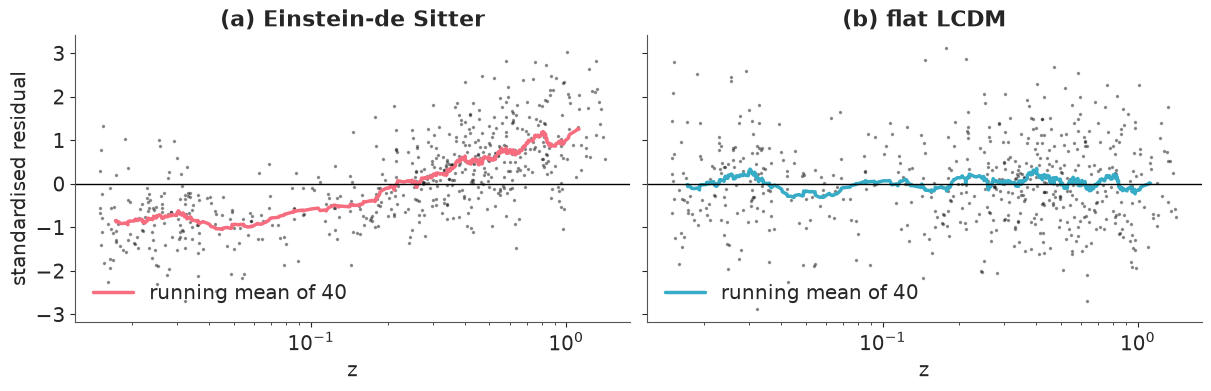
Einstein-de Sitter has a trend the offset cannot hide: nearby supernovae are brighter than predicted, distant ones fainter, because the offset can only shift the curve up and down to split the difference. Flat $\Lambda$CDM's running mean wobbles around zero with no trend (its excursions are what a mean of 40 unit-variance numbers does: $\pm 0.16$).
Now the proper posterior predictive version. For each model, simulate replicated datasets, reduce each to the 11 binned Hubble residuals relative to the empty universe, and ask whether the observed binned residuals look like a draw from that distribution.
with eds_model:
    pm.sample_posterior_predictive(eds_idata, extend_inferencedata=True, random_seed=RANDOM_SEED)
with flat_model:
    pm.sample_posterior_predictive(flat_idata, extend_inferencedata=True, random_seed=RANDOM_SEED)

fig, axes = plt.subplots(1, 2, figsize=(12, 4), sharey=True)
for ax, (label, idata, color) in zip(axes, [("(a) Einstein-de Sitter", eds_idata, "C1"),
                                            ("(b) flat LCDM", flat_idata, "C0")]):
    rep = az.extract(idata, group="posterior_predictive", var_names="mu_obs").transpose("sample", "sn").values
    rep_bin = binned_mean(rep - milne(z_obs))
    lo, hi = np.quantile(rep_bin, [0.03, 0.97], axis=0)
    ax.fill_between(z_bin, lo, hi, color=color, alpha=0.35, label="94% of replicated datasets")
    ax.plot(z_bin, rep_bin.mean(0), color=color)
    ax.plot(z_bin, resid_bin, "ko", ms=5, label="observed")
    ax.axhline(0, color="k", lw=1)
    ax.set(xscale="log", xlabel="z (bin mean)", title=label)
    ax.legend(loc="lower left")
    print(f"{label}: {int(((resid_bin < lo) | (resid_bin > hi)).sum())} of {n_bins} observed bins outside the 94% band")
axes[0].set(ylabel=r"binned $\mu - \mu_\mathrm{empty}$ (mag)");
(a) Einstein-de Sitter: 9 of 11 observed bins outside the 94% band
(b) flat LCDM: 0 of 11 observed bins outside the 94% band
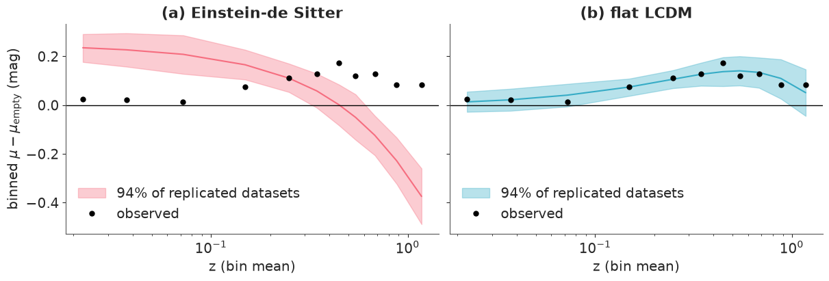
This is the 1998 discovery in one figure. The observed points rise above the empty universe out to $z \approx 0.5$ - supernovae are fainter than even a coasting universe allows - and then turn over. A matter-only universe can only ever go down; even with its inflated scatter and its 0.25 mag offset, most observed bins fall outside its predictive band, in a systematic pattern (the model sits above the data at low $z$ and far below at high $z$). Flat $\Lambda$CDM tracks the rise and the turn-over.
Heavy tails?
Supernova samples contain the odd misclassified or dust-reddened object, and a Gaussian likelihood lets one bad point drag the fit. The standard robustness check is a Student-t likelihood with the degrees of freedom $\nu$ free.
with pm.Model(coords=coords) as flat_t_model:
    Om = pm.Uniform("Om", 0.0, 1.0)
    hubble_likelihood(mu_shape(z_obs, Om, 1 - Om, xp=pt), student_t=True)
    flat_t_idata = pm.sample(**SAMPLE_KWARGS)

print("divergences:", int(flat_t_idata.sample_stats["diverging"].sum()))
az.summary(flat_t_idata, var_names=["Om", "offset", "sigma_int", "nu"], round_to=3)
divergences: 0
| mean | sd | eti89_lb | eti89_ub | ess_bulk | ess_tail | r_hat | mcse_mean | mcse_sd | |
|---|---|---|---|---|---|---|---|---|---|
| Om | 0.280 | 0.020 | 0.248 | 0.312 | 1568.121 | 1963.068 | 1.000 | 0.001 | 0.000 |
| offset | -0.000 | 0.011 | -0.018 | 0.017 | 1583.760 | 1746.168 | 1.000 | 0.000 | 0.000 |
| sigma_int | 0.015 | 0.011 | 0.001 | 0.036 | 1399.791 | 1073.486 | 1.002 | 0.000 | 0.000 |
| nu | 36.790 | 14.735 | 18.621 | 62.861 | 2671.932 | 2551.646 | 1.001 | 0.293 | 0.364 |
$\nu$ lands in the tens - essentially Gaussian - and $\Omega_m$ does not move. The heavy tails are not needed; the compilation has evidently already been through outlier rejection. We carry the Student-t model into the LOO table as a check and otherwise keep the Normal likelihood.
(c) Curved $\Lambda\text{CDM}$: the banana
Drop the flatness assumption and let $\Omega_m$ and $\Omega_\Lambda$ vary independently. Physics gives $\Omega_m \ge 0$ but does not bound $\Omega_\Lambda$ (a negative cosmological constant is perfectly legal), so we use a generous box.
One corner of that box is unphysical in an interesting way: for large $\Omega_\Lambda$ and
small $\Omega_m$, $E(z)^2$ goes negative at some redshift - a universe that bounced and
never had a Big Bang. comoving_distance clips $E^2$ at a tiny positive number there, which
makes the predicted distances absurdly large and the likelihood correspondingly terrible,
so the sampler stays away. We check afterwards that it did.
We take 2000 draws per chain here and in (d): two-dimensional contours of a curved posterior need more draws than a marginal mean does.
with pm.Model(coords=coords) as curved_model:
    Om = pm.Uniform("Om", 0.0, 1.5)
    OL = pm.Uniform("OL", -1.0, 2.0)
    pm.Deterministic("Ok", 1 - Om - OL)
    pm.Deterministic("q0", Om / 2 - OL)
    hubble_likelihood(mu_shape(z_obs, Om, OL, xp=pt))
    curved_idata = pm.sample(draws=2000, **SAMPLE_KWARGS)

print("divergences:", int(curved_idata.sample_stats["diverging"].sum()))
az.summary(curved_idata, var_names=["Om", "OL", "Ok", "q0", "offset", "sigma_int"], round_to=3)
divergences: 0
| mean | sd | eti89_lb | eti89_ub | ess_bulk | ess_tail | r_hat | mcse_mean | mcse_sd | |
|---|---|---|---|---|---|---|---|---|---|
| Om | 0.277 | 0.070 | 0.161 | 0.384 | 1767.439 | 2034.933 | 1.002 | 0.002 | 0.001 |
| OL | 0.718 | 0.118 | 0.522 | 0.901 | 1544.954 | 2080.537 | 1.002 | 0.003 | 0.002 |
| Ok | 0.005 | 0.184 | -0.277 | 0.311 | 1567.629 | 1912.003 | 1.001 | 0.005 | 0.003 |
| q0 | -0.579 | 0.088 | -0.717 | -0.434 | 1593.507 | 2322.729 | 1.001 | 0.002 | 0.001 |
| offset | 0.001 | 0.014 | -0.021 | 0.022 | 2217.560 | 3039.687 | 1.001 | 0.000 | 0.000 |
| sigma_int | 0.018 | 0.013 | 0.002 | 0.041 | 2500.197 | 1801.674 | 1.004 | 0.000 | 0.000 |
curved_post = az.extract(curved_idata)
z_fine = np.linspace(0, z_obs.max(), 200)

box = rng.uniform([0.0, -1.0], [1.5, 2.0], size=(20_000, 2))
no_big_bang_prior = (E2(z_fine, box[:, :1], box[:, 1:]) <= 0).any(axis=1).mean()
E2_post = E2(z_fine, curved_post["Om"].values[:, None], curved_post["OL"].values[:, None])
print(f"share of the prior box with E^2 <= 0 inside the data range: {no_big_bang_prior:.1%}")
print(f"share of posterior draws with E^2 <= 0 anywhere           : {(E2_post <= 0).any(axis=1).mean():.1%}")
print(f"posterior correlation of Om and OL: {np.corrcoef(curved_post['Om'], curved_post['OL'])[0, 1]:.2f}")
share of the prior box with E^2 <= 0 inside the data range: 4.2%
share of posterior draws with E^2 <= 0 anywhere           : 0.0%
posterior correlation of Om and OL: 0.90
def hdr_contours(ax, x, y, color, levels=(0.95, 0.68), grid=120, **kwargs):
    """Highest-density-region contours enclosing the given posterior masses (Gaussian KDE)."""
    kde = stats.gaussian_kde(np.vstack([x, y]))
    xx, yy = np.meshgrid(np.linspace(x.min(), x.max(), grid), np.linspace(y.min(), y.max(), grid))
    dens = kde(np.vstack([xx.ravel(), yy.ravel()])).reshape(xx.shape)
    dens_at_draws = np.sort(kde(np.vstack([x[::4], y[::4]])))
    cuts = [dens_at_draws[int((1 - level) * len(dens_at_draws))] for level in levels]
    ax.contourf(xx, yy, dens, levels=[*cuts, np.inf], colors=[color], alpha=0.3, **kwargs)
    ax.contour(xx, yy, dens, levels=cuts, colors=[color], linewidths=1.2)


om_line = np.linspace(0, 1.5, 50)
flat_lo, flat_hi = np.quantile(flat_post["Om"].values, [0.03, 0.97])

fig, ax = plt.subplots(figsize=(6.5, 6))
hdr_contours(ax, curved_post["Om"].values, curved_post["OL"].values, "C2")
ax.plot(om_line, 1 - om_line, "k-", lw=1, label=r"flat: $\Omega_\Lambda = 1 - \Omega_m$")
ax.plot(om_line, om_line / 2, "k--", lw=1, label=r"$q_0 = 0$: $\Omega_\Lambda = \Omega_m/2$")
ax.plot([flat_lo, flat_hi], [1 - flat_lo, 1 - flat_hi], color="C0", lw=5, solid_capstyle="butt",
        label="model (b), 94% interval")
ax.axhline(0, color="k", lw=0.5)
ax.plot(1, 0, "s", color="C1", ms=8, label="Einstein-de Sitter")
ax.text(0.76, 0.43, "accelerating", rotation=24, fontsize=9)
ax.text(0.80, 0.31, "decelerating", rotation=24, fontsize=9)
ax.set(xlim=(0, 1.05), ylim=(-0.15, 1.25), xlabel=r"$\Omega_m$", ylabel=r"$\Omega_\Lambda$",
       title="Curved LCDM: 68% and 95% posterior regions")
ax.legend(loc="lower right", fontsize=8);
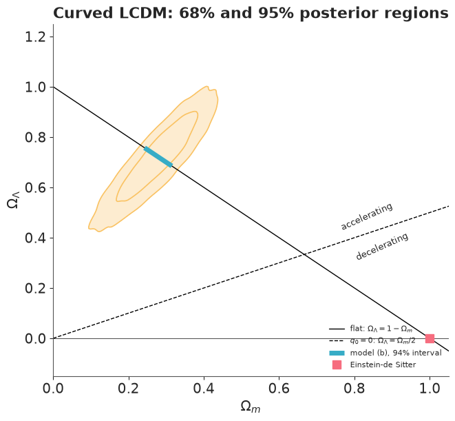
The famous picture. Supernovae do not measure $\Omega_m$ and $\Omega_\Lambda$ separately: they measure, roughly, the difference between brake and accelerator, so the posterior is a long diagonal ridge - the two are correlated at about 0.9 - and the marginal uncertainties are 3.5 times ($\Omega_m$) and 6 times ($\Omega_\Lambda$) what they were in the flat model. Unlike the $H_0$-$M$ ridge, this one is a soft degeneracy: it has finite length because the redshift lever arm distinguishes the two terms a little, and NUTS handles it without complaint.
What the banana does and does not say:
- It lies entirely above the dashed $q_0 = 0$ line and above $\Omega_\Lambda = 0$. Acceleration does not depend on assuming flatness.
- It is consistent with flat: the solid line runs through the middle, and $\Omega_k = 0$ is well inside its posterior. But supernovae alone constrain curvature poorly ($\pm 0.2$); it is the CMB that nails flatness, which is why combining probes whose degeneracy directions cross is so powerful.
- Einstein-de Sitter is nowhere near.
(d) Flat $w\text{CDM}$: is dark energy a cosmological constant?
Keep flatness, free the equation of state. The prior $w \sim \text{Uniform}(-3, 0)$ is deliberately agnostic: it includes "phantom" dark energy ($w < -1$) and components that would not accelerate anything ($w > -1/3$).
with pm.Model(coords=coords) as wcdm_model:
    Om = pm.Uniform("Om", 0.0, 1.0)
    w = pm.Uniform("w", -3.0, 0.0)
    pm.Deterministic("q0", 0.5 + 1.5 * w * (1 - Om))
    hubble_likelihood(mu_shape(z_obs, Om, 1 - Om, w, xp=pt))
    wcdm_idata = pm.sample(draws=2000, **SAMPLE_KWARGS)

print("divergences:", int(wcdm_idata.sample_stats["diverging"].sum()))
az.summary(wcdm_idata, var_names=["Om", "w", "q0", "offset", "sigma_int"], round_to=3)
divergences: 0
| mean | sd | eti89_lb | eti89_ub | ess_bulk | ess_tail | r_hat | mcse_mean | mcse_sd | |
|---|---|---|---|---|---|---|---|---|---|
| Om | 0.275 | 0.076 | 0.135 | 0.381 | 1301.812 | 1216.097 | 1.004 | 0.002 | 0.002 |
| w | -1.030 | 0.203 | -1.362 | -0.720 | 1238.854 | 1231.144 | 1.005 | 0.006 | 0.004 |
| q0 | -0.598 | 0.114 | -0.787 | -0.426 | 1330.264 | 1639.679 | 1.004 | 0.003 | 0.002 |
| offset | -0.001 | 0.015 | -0.025 | 0.023 | 1954.683 | 2768.183 | 1.002 | 0.000 | 0.000 |
| sigma_int | 0.018 | 0.013 | 0.002 | 0.041 | 2469.331 | 2123.504 | 1.002 | 0.000 | 0.000 |
wcdm_post = az.extract(wcdm_idata)
om_line = np.linspace(0, 0.6, 100)

fig, ax = plt.subplots(figsize=(6.5, 4.8))
hdr_contours(ax, wcdm_post["Om"].values, wcdm_post["w"].values, "C3")
ax.axhline(-1, color="k", lw=1, label=r"cosmological constant, $w=-1$")
ax.plot(om_line, -1 / (3 * (1 - om_line)), "k--", lw=1, label=r"$q_0 = 0$")
ax.plot([flat_lo, flat_hi], [-1, -1], color="C0", lw=5, solid_capstyle="butt", label="model (b), 94% interval")
ax.set(xlim=(0, 0.6), ylim=(-2.2, 0), xlabel=r"$\Omega_m$", ylabel="w",
       title="Flat wCDM: 68% and 95% posterior regions")
ax.legend(loc="upper left", fontsize=8);
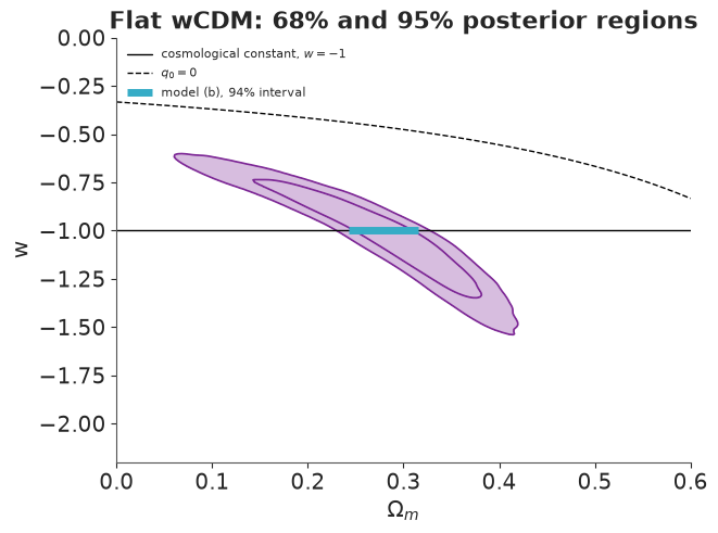
Another banana, this time genuinely bent: more matter can be compensated by more negative pressure. $w = -1$ passes straight through the middle, so the data are perfectly happy with a cosmological constant - but on their own they allow anything from about $-1.4$ to $-0.7$, and the 95% region stretches from $\Omega_m < 0.1$ to above 0.4. The whole posterior stays below the $q_0 = 0$ curve. An external constraint on $\Omega_m$ (BAO, CMB) would slice the banana vertically and tighten $w$ dramatically - see Try it yourself.
LOO: which universe predicts held-out supernovae best?
idatas = {"(a) Einstein-de Sitter": (eds_model, eds_idata), "(b) flat LCDM": (flat_model, flat_idata),
          "(b') flat LCDM, Student-t": (flat_t_model, flat_t_idata),
          "(c) curved LCDM": (curved_model, curved_idata), "(d) flat wCDM": (wcdm_model, wcdm_idata)}
for model, idata in idatas.values():
    with model:
        pm.compute_log_likelihood(idata, progressbar=False)

comparison = az.compare({name: idata for name, (_, idata) in idatas.items()}, round_to=1)
comparison
| rank | elpd_diff | dse | p_worse | diag_diff | diag_elpd | p | elpd | se | weight | |
|---|---|---|---|---|---|---|---|---|---|---|
| (b) flat LCDM | 0 | 0.0 | 0.0 | NaN | 1.9 | 116.3 | 20.3 | 1.0 | ||
| (b') flat LCDM, Student-t | 1 | -0.8 | 1.0 | 0.8 | |elpd_diff| < 4 | 1.9 | 115.5 | 19.7 | 0.0 | |
| (d) flat wCDM | 2 | -0.9 | 0.1 | 1.0 | |elpd_diff| < 4 | 2.8 | 115.4 | 20.3 | 0.0 | |
| (c) curved LCDM | 3 | -1.0 | 0.1 | 1.0 | |elpd_diff| < 4 | 2.8 | 115.4 | 20.3 | 0.0 | |
| (a) Einstein-de Sitter | 4 | -219.6 | 16.9 | 1.0 | 2.0 | -103.3 | 19.7 | 0.0 |
az.plot_compare(comparison);
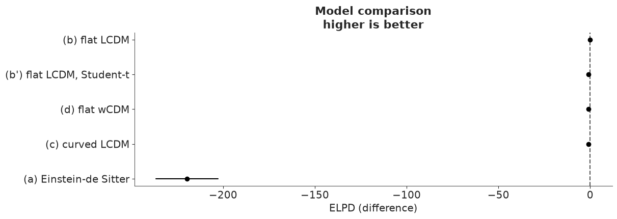
Two very different verdicts, and both matter:
- Einstein-de Sitter is out, by more than 200 units of elpd - over ten standard errors of the difference. Note this is after it was allowed to inflate $\sigma_\text{int}$ to protect itself; without that freedom it would look far worse. Here LOO is answering a physics question: a universe with only matter in it does not predict supernova brightnesses, and one with a cosmological constant does.
- Among the dark-energy models LOO cannot choose, and says so: the differences are
below one unit, far inside the $|\text{elpd\_diff}| < 4$ zone where ArviZ itself warns
against reading anything into the ranking. Curvature and $w$ each cost about one
effective parameter (
p) and buy no predictive accuracy. That is not evidence that the universe is flat or that $w=-1$; it says these data cannot tell, which is exactly what the two bananas showed. The simplest adequate model is (b).
7 · From posterior to scientific answers
Parameters with physical meaning can be pushed through more physics, draw by draw.
Is the expansion accelerating? $P(q_0 < 0)$ under each dark-energy model:
q0_draws = {
    "(b) flat LCDM": 1.5 * flat_post["Om"].values - 1,
    "(c) curved LCDM": curved_post["q0"].values,
    "(d) flat wCDM": wcdm_post["q0"].values,
}
answers = pd.DataFrame({
    name: {"q0 mean": q.mean(), "q0 3%": np.quantile(q, 0.03), "q0 97%": np.quantile(q, 0.97),
           "largest q0 drawn": q.max(), "draws": len(q), "P(q0 < 0)": (q < 0).mean()}
    for name, q in q0_draws.items()
}).T
answers.round(3)
| q0 mean | q0 3% | q0 97% | largest q0 drawn | draws | P(q0 < 0) | |
|---|---|---|---|---|---|---|
| (b) flat LCDM | -0.582 | -0.636 | -0.527 | -0.461 | 4000.0 | 1.0 |
| (c) curved LCDM | -0.579 | -0.740 | -0.408 | -0.207 | 8000.0 | 1.0 |
| (d) flat wCDM | -0.598 | -0.823 | -0.404 | -0.286 | 8000.0 | 1.0 |
fig, ax = plt.subplots(figsize=(8, 3.5))
for (name, q), color in zip(q0_draws.items(), ["C0", "C2", "C3"]):
    ax.hist(q, bins=60, density=True, histtype="stepfilled", alpha=0.35, color=color, label=name)
ax.axvline(0, color="k", lw=1)
ax.axvline(0.5, color="C1", lw=2, label="Einstein-de Sitter")
ax.set(xlabel=r"deceleration parameter $q_0$", yticks=[], title="Negative = accelerating")
ax.legend(fontsize=8);
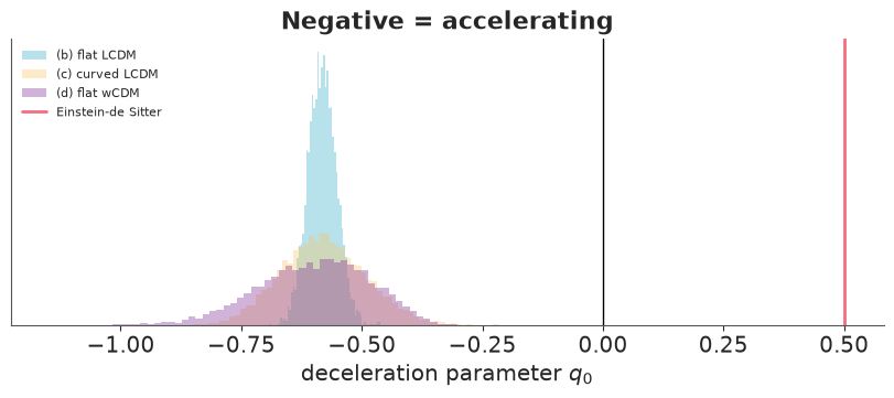
Not a single posterior draw in any of the three models decelerates, so all a Monte Carlo estimate can honestly say is that $P(\text{accelerating})$ exceeds $1 - 1/\text{draws}$. Relaxing flatness or $w = -1$ widens $q_0$ by a factor of three to four but leaves it centred near $-0.6$, many standard deviations from zero.
That probability is conditional on everything we assumed: a homogeneous universe obeying general relativity, supernovae that are the same kind of candle at $z = 1$ as nearby, and
- importantly - the error model discussed in section 8.
How much dark energy, when did acceleration begin, and how old is the universe? For $w = -1$, $\ddot a = 0$ when $\Omega_m (1+z)^3 = 2\,\Omega_\Lambda$, so the transition redshift is $z_t = (2\Omega_\Lambda/\Omega_m)^{1/3} - 1$. The age is one more integral,
$$t_0 = \frac{1}{H_0}\int_0^1 \frac{da}{a\,E(a)} = \frac{1}{H_0}\int_0^1 \frac{2u^2\,du}{\sqrt{\Omega_m + \Omega_k u^2 + \Omega_\Lambda u^6}} \qquad (a = \tfrac{1}{1+z} = u^2),$$
where the substitution removes the square-root singularity at the Big Bang so that Gauss-Legendre converges fast. No gradients are needed now, so this is plain NumPy on the posterior draws. It needs an $H_0$, which - section 4 - supernovae cannot supply: we condition on $h = 0.7$, and $t_0$ scales as $1/h$.
KM_PER_MPC, SEC_PER_GYR = 3.0856775814913673e19, 3.15576e16
HUBBLE_TIME_GYR = KM_PER_MPC / H0_FID / SEC_PER_GYR  # 1/H0 for h = 0.7


def age_gyr(Om, OL, n_nodes=32):
    """Age of a w = -1 universe in Gyr for h = 0.7; Om, OL are arrays of posterior draws."""
    x_k, w_k = np.polynomial.legendre.leggauss(n_nodes)
    u = 0.5 * (x_k + 1)
    Om, OL = Om[..., None], OL[..., None]
    integrand = 2 * u**2 / np.sqrt(Om + (1 - Om - OL) * u**2 + OL * u**6)
    return HUBBLE_TIME_GYR * 0.5 * (w_k * integrand).sum(-1)


# check: quad on the un-substituted integral, and the closed form for a flat universe
quad_age = HUBBLE_TIME_GYR * integrate.quad(lambda a: 1 / np.sqrt(0.3 / a + 0.7 * a**2), 0, 1)[0]
closed_form = HUBBLE_TIME_GYR * 2 / (3 * np.sqrt(0.7)) * np.arcsinh(np.sqrt(0.7 / 0.3))
print(f"1/H0 = {HUBBLE_TIME_GYR:.2f} Gyr;  age(Om=0.3, flat): quadrature {age_gyr(np.array(0.3), np.array(0.7)):.4f}, "
      f"quad {quad_age:.4f}, closed form {closed_form:.4f} Gyr")

Om_flat = flat_post["Om"].values
derived = {
    r"Omega_Lambda": 1 - Om_flat,
    r"q0": 1.5 * Om_flat - 1,
    r"transition redshift z_t": (2 * (1 - Om_flat) / Om_flat) ** (1 / 3) - 1,
    r"age (Gyr), given h = 0.7": age_gyr(Om_flat, 1 - Om_flat),
    r"age in units of 1/H0": age_gyr(Om_flat, 1 - Om_flat) / HUBBLE_TIME_GYR,
}
pd.DataFrame({k: {"mean": v.mean(), "sd": v.std(), "3%": np.quantile(v, 0.03), "97%": np.quantile(v, 0.97)}
              for k, v in derived.items()}).T.round(3)
1/H0 = 13.97 Gyr; age(Om=0.3, flat): quadrature 13.4670, quad 13.4670, closed form 13.4670 Gyr
| mean | sd | 3% | 97% | |
|---|---|---|---|---|
| Omega_Lambda | 0.721 | 0.020 | 0.685 | 0.757 |
| q0 | -0.582 | 0.029 | -0.636 | -0.527 |
| transition redshift z_t | 0.732 | 0.056 | 0.632 | 0.841 |
| age (Gyr), given h = 0.7 | 13.758 | 0.268 | 13.284 | 14.276 |
| age in units of 1/H0 | 0.985 | 0.019 | 0.951 | 1.022 |
Under flat $\Lambda\text{CDM}$: dark energy is about 72% of the universe; the expansion switched from slowing down to speeding up at $z_t \approx 0.73$ - inside the redshift range of the data, which is why the turn-over in the residual plot is visible at all - and the universe is about 13.8 billion years old if $h = 0.7$. The last row is the assumption-free version of that statement: the age is $0.985 \pm 0.02$ Hubble times. (For Einstein-de Sitter it would be exactly $2/3$ of a Hubble time, 9.3 Gyr for $h = 0.7$ - younger than the oldest stars, one of the pre-1998 hints that something was missing.)
The four universes, and the extrapolation
Posterior mean and 94% band of each model's curve (with its own offset) against the binned data, continued beyond the last supernova.
def residual_curves(post, Om, OL, w=-1.0, n=1000):
    """Posterior draws of mu(z_grid) - mu_empty(z_grid), including each draw's offset."""
    idx = rng.choice(post.sizes["sample"], size=n, replace=False)
    pick = lambda p: p[idx, None] if np.ndim(p) else p
    return mu_shape(z_grid, pick(Om), pick(OL), pick(w)) + MU0_FID + post["offset"].values[idx, None] - milne(z_grid)


eds_post = az.extract(eds_idata)
curves = {
    "(a) Einstein-de Sitter": (residual_curves(eds_post, 1.0, 0.0), "C1"),
    "(b) flat LCDM": (residual_curves(flat_post, Om_flat, 1 - Om_flat), "C0"),
    "(c) curved LCDM": (residual_curves(curved_post, curved_post["Om"].values, curved_post["OL"].values), "C2"),
    "(d) flat wCDM": (residual_curves(wcdm_post, wcdm_post["Om"].values, 1 - wcdm_post["Om"].values,
                                      wcdm_post["w"].values), "C3"),
}

fig, ax = plt.subplots(figsize=(9, 4.8))
for (name, (curve, color)), ls in zip(curves.items(), ["-", "-", "--", ":"]):
    lo, hi = np.quantile(curve, [0.03, 0.97], axis=0)
    ax.fill_between(z_grid, lo, hi, color=color, alpha=0.2)
    ax.plot(z_grid, curve.mean(0), color=color, ls=ls, lw=2, label=name)
ax.errorbar(z_bin, resid_bin, yerr=resid_bin_se, fmt="ko", ms=4, label="data, binned (published errors)")
ax.axhline(0, color="k", lw=1)
ax.axvspan(z_obs.max(), z_grid.max(), color="k", alpha=0.06)
ax.text(1.5, 0.27, "no data:\nextrapolation", fontsize=9)
ax.set(xlim=(0, 2.5), ylim=(-1.0, 0.4), xlabel="z", ylabel=r"$\mu - \mu_\mathrm{empty}$ (mag)",
       title="Hubble residuals relative to an empty universe")
ax.legend(loc="lower left", fontsize=8);
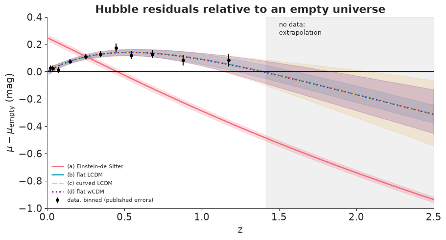
Inside the data the three dark-energy models are indistinguishable - as LOO said. Beyond $z = 1.4$ they are still all physically sensible curves: each bends back down, because in any of these universes matter dominated early on and the expansion was decelerating. The bands widen in the grey region, the more flexible models more so, and that widening is itself informative: it says precisely which future observations ($z > 1.5$ supernovae) would discriminate between them. A spline or polynomial fitted to the same points has no such anchor: nothing in it knows that matter must win at early times.
8 · What we did not model
- Systematics. We used only the diagonal
mu_err. The real analysis has a full $580 \times 580$ covariance matrix: calibration, dust and light-curve-model uncertainties shift groups of supernovae together, which is far more damaging to a measurement of shape than independent noise. In the Union2.1 paper, including it roughly doubles the uncertainty on $\Omega_m$. Our intervals are too narrow, and statements like "many standard deviations from zero" should be read with that in mind (the qualitative conclusions survive). With the matrix in hand the change to the model is small:pm.MvNormalwith the full covariance in place ofpm.Normal. - The standardisation itself. The published $\mu$ are the output of a light-curve fit (stretch and colour corrections) whose coefficients were estimated together with a cosmology. A fully Bayesian treatment models light-curve parameters and cosmology jointly, hierarchically.
- Astrophysics. Supernovae in low-mass host galaxies are slightly fainter after
standardisation; the column
p_low_mass_hostis there to model it (below).
Recap
| Theory as regression function | one function mu_shape, four models as constraints on it; parameters you can look up in a textbook |
| Integral inside the model | fixed-order Gauss-Legendre in plain PyTensor arithmetic; verified against quad to $10^{-14}$ mag; a power series instead of branching for $\text{sinn}$ |
| What went wrong | $H_0$ and $M$ are exactly degenerate: bad r_hat, posterior = prior along a ridge. Fix the model (sample the identified combination), not the sampler |
| Misfit sponge | Einstein-de Sitter sampled perfectly and hid its failure in $\sigma_\text{int}$; residuals against $z$ exposed it |
| Soft degeneracies | the $(\Omega_m,\Omega_\Lambda)$ and $(\Omega_m, w)$ bananas are real features of what the data can say - report them, do not fight them |
| LOO | decisive where the physics differs (matter-only vs dark energy), honest where the data cannot tell (curvature, $w$) |
Try it yourself
- Host-mass step. Add a term $\Delta_\text{host}\cdot$
p_low_mass_hosttomuinhubble_likelihood(the column is the probability that the host galaxy has low stellar mass). Is $\Delta_\text{host}$ distinguishable from zero, which sign does it have, and does $\Omega_m$ move? Think about why a population drift with redshift would matter. - Break the $w$ degeneracy with an external probe. Replace the uniform prior on
$\Omega_m$ in model (d) by an informative Gaussian standing in for BAO + CMB, say
pm.Normal("Om", 0.30, 0.02)truncated to $(0, 1)$. How much does the interval on $w$ shrink? Redraw the banana with the old one behind it. - Time-varying dark energy. Implement the CPL parametrisation
$w(a) = w_0 + w_a(1-a)$, for which the dark-energy term in $E(z)^2$ becomes
$\Omega_\Lambda (1+z)^{3(1+w_0+w_a)}\exp\!\big(-3 w_a z/(1+z)\big)$. Only
E2needs to change. Expect the sampler to work hard: look at the $(w_0, w_a)$ pair plot, checkr_hat, and decide what prior information on $w_a$ you can defend.
Next: E09, where the numerics are too involved for plain PyTensor and come in through
pytensor.wrap_jax instead.