A Hawkes Process Is a Poisson Process Whose Events Cause More Events

A Poisson process has no memory. Its rate at any moment ignores everything that has already happened, so one event tells you nothing about when the next will come. Earthquakes do not behave that way. After a large one the rate of smaller ones jumps by orders of magnitude and then decays, and each aftershock has aftershocks of its own.

A model in which every event raises the probability of further events is called self-exciting. The simplest is the Hawkes process (Hawkes 1971). Its seismological version, the Epidemic-Type Aftershock Sequence model or ETAS (Ogata 1988), is the workhorse of operational aftershock forecasting. I built a worked example on the 2019 Ridgecrest sequence in California: an M6.4 on 4 July, then an M7.1 34 hours later and 12 km away. The data are 6,909 earthquakes of magnitude 2.0 or more from the USGS catalogue of the surrounding box, 2016 to 2019. The question is the one that matters a day after the M7.1: what will the next week bring?

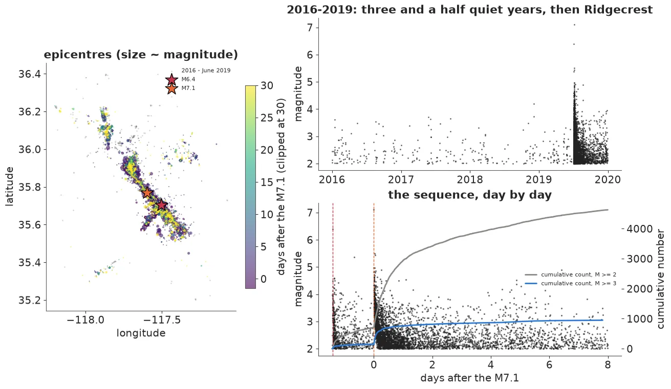
That figure is the notebook’s own plot of the catalogue. The box recorded 31 events of M3 or more in the three and a half years before the M6.4, 148 between the two large shocks, and 611 in the first day after the M7.1.

An intensity that remembers

A point process in time is described by its conditional intensity $\lambda(t \mid \mathcal{H}_t)$: the expected number of events per unit time at $t$, given the history of everything before $t$. A Poisson process has an intensity that ignores the history. A Hawkes process adds a bump for every past event:

$\lambda(t) = \mu + \sum_{t_j < t} \kappa\, g(t - t_j), \qquad \int_0^\infty g(s)\,ds = 1$

Here $\mu$ is the background rate, $g$ is the triggering kernel that says how the extra rate decays, and $\kappa$ is the expected number of events that each event triggers directly.

The same equation has a second reading, the branching representation. Background events arrive as a Poisson process. Each event then has a Poisson($\kappa$) number of children at delays drawn from $g$, the children have children, and so on. That is how the figure was simulated, and it is also how the forecast below is made.

Why the branching ratio must stay below one

$\kappa$ is the branching ratio, usually written $n$. One background event has $n$ children on average, $n^2$ grandchildren, and a mean family of

$1 + n + n^2 + \dots = \frac{1}{1 - n}$

The series converges only if $n < 1$. With $n \ge 1$ a cascade can run forever and the process has no stationary rate. Below one, the long-run rate is $\mu / (1 - n)$ and the share of events that are background is $1 - n$. At $n = 0.8$ only a fifth of the events are spontaneous. The rest are descendants, which is why counts from a Hawkes process are overdispersed.

What ETAS adds

ETAS is a Hawkes process with magnitudes. For events above a completeness magnitude $M_c$,

$\lambda(t) = \mu + \sum_{t_j < t} K_0\, e^{\alpha (m_j - M_c)}\,(t - t_j + c)^{-p}$

It changes three things. The kernel is the Omori-Utsu power law $(t + c)^{-p}$, where the short delay $c$ keeps the rate finite at zero and $p$ is about 1. Productivity grows with size: an event one magnitude unit bigger has $e^{\alpha}$ times more direct aftershocks. And magnitudes follow the Gutenberg-Richter law, exponential with rate $\beta = b \ln 10$ and independent of the past.

The branching ratio is now an average over magnitudes, $n = K_0\, G(\infty)\, \mathbb{E}[e^{\alpha (m - M_c)}]$, where $G(\infty)$ is the kernel’s total mass and is finite only for $p > 1$. As $\alpha$ approaches $\beta$ the expectation is dominated by the rare largest events, so stability is a contest between productivity and the b-value. Under the priors about 60% of draws had $n \ge 1$ or $p \le 1$. I did not force $n < 1$, because a short, intense sequence can look near-critical.

The likelihood, and the trick that makes it affordable

For events at times $t_i$ with magnitudes $m_i$ observed on $[S, T]$, the log-likelihood is

$\log L = \sum_i \log \lambda(t_i) - \int_S^T \lambda(t)\,dt + \sum_i \log f_{GR}(m_i)$

The first term rewards a high rate where events happened. The integral, called the compensator, charges for a high rate everywhere else. It has a closed form, because each event’s kernel integrates analytically, and it costs $O(n)$. The first sum is the expensive part: every $\lambda(t_i)$ involves every earlier event. The Ridgecrest fit has 790 parent events, which is 311,655 pairs per gradient evaluation.

An exponential kernel has a classic way out. With $A_i = \sum_{j < i} w_j e^{-(t_i - t_j)/c}$, the sum updates in one step, $A_i = e^{-(t_i - t_{i-1})/c}(A_{i-1} + w_{i-1})$. A power law has no such recursion, but it is a mixture of exponentials:

$(x + c)^{-p} = \frac{1}{\Gamma(p)} \int_0^\infty s^{p-1} e^{-sc}\, e^{-sx}\, ds \approx \sum_{k=1}^{K} w_k(c, p)\, e^{-s_k x}$

The nodes $s_k$ sit on a fixed grid in $\log s$, so the decay factors between consecutive events are constants. The parameters $c$ and $p$ enter only through the weights. The recursion runs on a vector of $K = 79$ states and costs $O(nK)$.

In PyMC it is one pytensor.scan and two potentials. Here ea is the productivity of every event, tgt indexes the events in the likelihood, and comp is the closed-form compensator:

U_NODES = np.arange(-25.0, 14.0 + 1e-9, 0.5)     # log s nodes
sk = np.exp(U_NODES)
decay = np.exp(-np.outer(np.diff(t), sk))        # fixed: (n - 1) x K
wk = pt.exp(p * U_NODES - sk * c - pt.gammaln(p)
            + np.log(U_NODES[1] - U_NODES[0]))
A = pytensor.scan(lambda dec, e, a: dec * (a + e),
                  sequences=[pt.as_tensor(decay), ea[:-1]],
                  outputs_info=[pt.zeros(len(sk))], return_updates=False)
A = pt.concatenate([pt.zeros((1, len(sk))), A], axis=0)
lam = mu + K0 * (A @ wk)[tgt]

pm.Potential("time_loglik", pt.log(lam).sum() - comp)
pm.Potential("magnitude_loglik",
             (pt.log(beta) - beta * dm[tgt] - pt.log(Z)).sum())

On the Ridgecrest events the mixture gave a log-density of 1407.57630 against 1407.57631 for the exact pair sum, at 0.41 ms per gradient instead of 3.97 ms. The gap widens with the catalogue.

The catalogue is incomplete exactly when it matters

Right after a large earthquake, seismograms are saturated and small events disappear under the coda of big ones. In the first 15 minutes after the M7.1 the most common recorded magnitude was 4, and the b-value above M3 came out at 0.40, against about 1.1 before the sequence. The physics did not change. Most M3s were never catalogued.

A model fitted as if the catalogue were complete sees too few early events and explains the shortfall the only ways it can: a larger $c$, a different $p$, and a smaller b-value, which means more large earthquakes. The fix keeps the model of the true process and adds a model of the observation. An event enters the likelihood only if it is above a time-varying threshold $M_c(t)$ (the formula of Helmstetter, Kagan & Jackson 2006, in steps), and the compensator becomes $\int q(t) \lambda(t)\, dt$, where $q(t)$ is the Gutenberg-Richter probability that an event clears the threshold. Only the compensator changes.

I tested this first where the answer is known. In a simulated sequence of 788 events of which 427 were “recorded”, the naive fit put $c$ at about an hour instead of 3 minutes. The $M_c(t)$ fit covered the truth with its 90% interval for every parameter. That is one simulated sequence, so it shows the direction and size of the bias, not a calibration rate.

What the fit showed on Ridgecrest

Three models were fitted to everything up to 24 hours after the M7.1: naive ETAS with constant completeness, ETAS with $M_c(t)$, and an exponential-kernel Hawkes process with $M_c(t)$. All three sampled cleanly, with no divergences and r-hat at most 1.01. Clean is not the same as right.

The naive model repeated the simulated failure on real data: $c$ of about 25 minutes instead of about 2, $p$ of about 1.43 against 1.17, $\alpha$ of 2.0 against 2.3, and a b-value of about 0.87 against 1.07. A difference of 0.2 in $b$ is a factor of about 2.5 in the predicted share of M5+ among M3+ events. The exponential model cannot cover minutes to days with one time scale. Its memory settled near an hour and a half.

A goodness-of-fit check separated them. Under the time-rescaling theorem, the fitted compensator should turn the event times into a unit-rate Poisson process. A Kolmogorov-Smirnov test on the rescaled gaps rejected 82% of posterior draws for the naive model and 79% for the exponential one, against 2% for ETAS with $M_c(t)$.

For that model the branching ratio has a posterior median of 0.70 and a 90% interval of 0.45 to 1.19, with 12% of draws at or above one. Over one week that is not a contradiction, since a near-critical process still produces finite counts in 7 days, but it gives the forecast a long right tail.

The fitted intensity also says who triggered whom. The probability that the M7.1 was a background event is about 0.0001. Its direct parent was probably not the M6.4 (0.02) but an M5.0 that struck three minutes earlier (about 0.8). The M6.4 is among its ancestors with probability 0.99.

The forecast and the week that followed

For each of 1,000 posterior draws, the notebook simulates the next 7 days from the branching representation: the remaining aftershocks of every catalogued event, the background, and every later generation. The week itself was held out of every fit.

ETAS with $M_c(t)$ put the week at a median of 230 M3+ events (90% interval 151 to 566) and 20 M4+ (9 to 53). What happened was 191 and 12: inside the intervals and below the medians. It gave an M5 or larger a probability of 0.76, and the largest event was an M4.9. One week of one sequence cannot tell whether 0.76 was too high.

The naive model gave an earthquake larger than the M7.1 a probability of 0.117 within the week, about ten times the 0.012 of the model that accounts for missing events. That is not a cautious forecast. It is a wrong one, produced by the catalogue’s missing small events. The exponential model predicted a median of 5 events for a week that had 191. On the held-out log-likelihood the naive model scored 7.5 below ETAS with $M_c(t)$ and the exponential model 51.6 below.

The same model, refitted with only the data available 12 hours after the M6.4, gave an event at least that large within a week a probability of 0.075, and an M7 or larger 0.033. The M7.1 came 22 hours later. A 3% to 7% event happening once is not evidence against a 3% to 7% forecast. Only many sequences can test that.

Where it breaks

The sampler diagnostics never flagged the naive model. The failure was in the data model, and only the rescaling check and the forecast tails exposed it. The completeness fix has its own limit: every catalogued event still acts as a parent, but parents that were never recorded stay missing. In the simulation the 361 unrecorded parents hardly mattered, and that was one sequence. The model is also temporal only, and it treats local and moment magnitudes as one scale.

What to do in practice

1. Write the intensity first. Both likelihood terms follow from it: the sum of log intensities at the events, minus the integral.

2. Report the branching ratio as a posterior. State how much of it sits at or above one, because that decides the forecast’s tail.

3. Match the kernel to the decay. An exponential kernel has one time scale. A decay that spans minutes to days needs a power law, and the mixture of exponentials keeps it fast.

4. Model how the events were recorded. If detection changes over time, put the detection probability in the compensator.

5. Check the fit with time rescaling. Divergences and r-hat describe the sampler. They say nothing about whether the process matches the data.

6. Forecast by simulating cascades from posterior draws, and score on held-out data. A single rare outcome is not a verdict on a probability.

Further reading: the full worked example has the data, the complete model code, the declustering and the forecast figures. All empirical numbers above come from it. Its sampler is not bit-reproducible, so last digits move between runs. References, as cited there: Hawkes (1971), Ogata (1988), Helmstetter, Kagan & Jackson (2006). Data: USGS ANSS Comprehensive Catalog, public domain.