On 14 September 2015 the two LIGO detectors recorded a 0.2 second chirp from two black holes merging 1.3 billion light years away. The strain data are public. I built a worked example that asks what NumPy, SciPy and PyMC can learn from 32 seconds of them, sampled at 4096 Hz at Hanford (H1) and Livingston (L1).
The waveform I fit is one line of physics. The statistical work is in the noise. In units of , the raw strain has an rms of 218 at H1 and 231 at L1, and the signal peaks at about one. The noise is also strongly correlated from one sample to the next, so a normal likelihood with independent errors on the raw samples is the wrong model. This post is about what the right likelihood looks like and what it showed.
The example carries a caveat that applies here too. This is a simplified, pedagogical analysis: analytic toy waveforms, a noise model estimated from 30 seconds of data, no calibration uncertainty, no sky location. It is not a reproduction of the LIGO-Virgo analysis. Where a number agrees with a published one, the claim is “consistent with.”
Coloured noise
Noise is white when every frequency carries the same power, which is the same as saying its samples are uncorrelated. Detector noise is far from that. The power spectral density gives the noise variance per hertz. The example estimates it with Welch’s method, using only data more than 2 seconds from the event so the signal cannot leak into its own noise estimate.
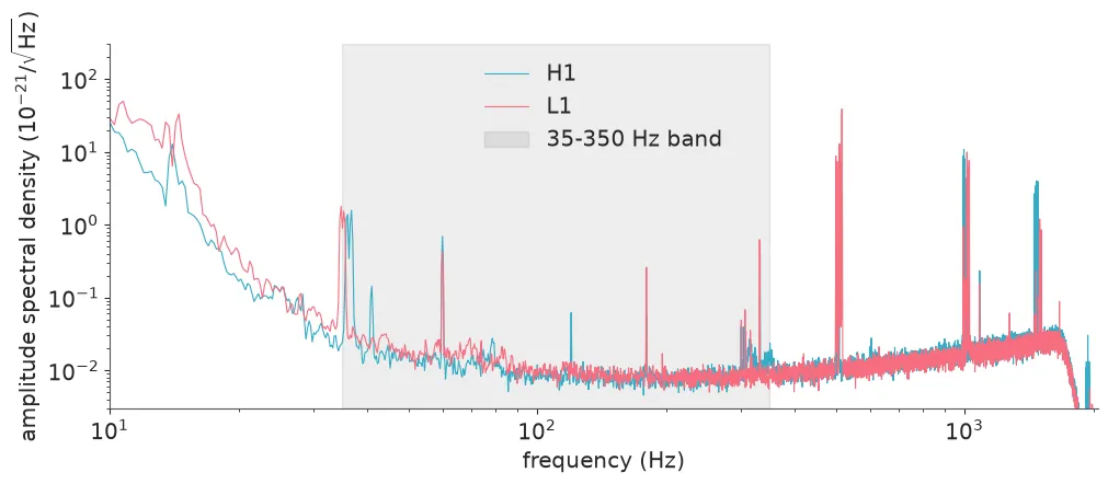
The amplitude spectral density falls by a factor of several thousand between 10 Hz and the quiet band near 100 to 300 Hz. On top sit narrow lines: mains harmonics at multiples of 60 Hz, suspension modes near 500 Hz, calibration lines. The slow wander that hides the event in the raw strain is the left edge of this plot.
What whitening does
If the noise is stationary and Gaussian, its Fourier coefficients at different frequencies are independent, with variance proportional to . For data and a template that gives the Whittle likelihood:
Whitening divides the Fourier transform of the data by . Every becomes equal: the loud low frequencies are turned down and the quiet band is turned up. By Parseval’s theorem the sum over frequencies is then a sum over time samples with unit variance. On the real data the whitened off-source standard deviation came out at 0.99 for H1 and 1.15 for L1, with the L1 excess sitting entirely below 10 Hz.
Whitened and band-passed to 35 to 350 Hz, the real strain shows the event:
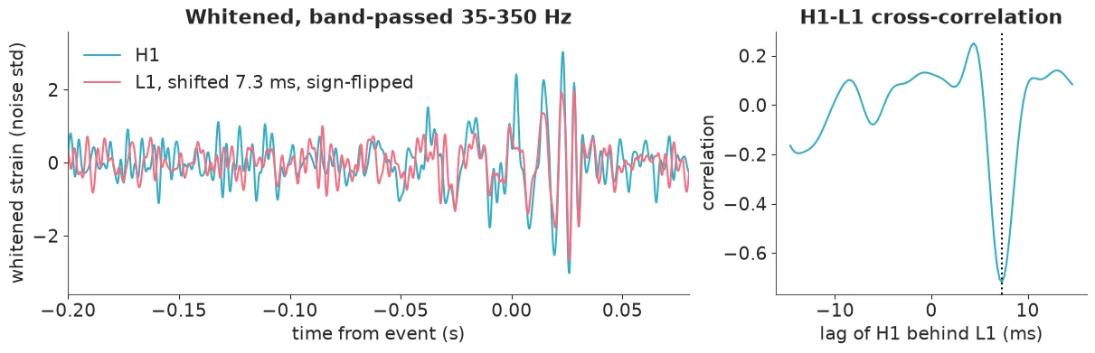
The same shape appears in two instruments 3000 km apart. A cross-correlation puts Livingston 7.3 ms ahead, with the opposite sign and a correlation of -0.72.
Three traps in the shortcut
Whitening suggests an easy likelihood: filter the data, then fit it with independent unit-variance normal errors. The example lists three ways that goes wrong.
- The template must be whitened too. The filter changes the shape of any signal, as the last step of the figure above shows. An unwhitened waveform does not fit whitened data.
- Band-passed samples are not independent. After the band-pass the noise has a standard deviation of 0.37 and neighbouring samples are strongly correlated. Setting
sigma = 0.37with independent samples counts the same information several times. - The filters are acausal and long. Whitening and zero-phase band-passing smear every feature over tens of milliseconds in both directions.
The third trap decides the design, because of which part of the signal has a closed-form model.
The waveform is the regression function
After the merger, the new black hole rings like a struck bell. Keeping only the dominant mode, the signal is a damped sinusoid:
Statistically this is the mean function of a nonlinear regression with a frequency, a damping time, an amplitude and a phase. It holds only after a start time , and the much louder merger sits just before it. An acausal filter carries merger power across into the window the model is supposed to explain.
An exact likelihood in the time domain
The fix, following Isi & Farr (2021), is to stay in the time domain. Stationary Gaussian noise is fully described by its autocovariance , the inverse Fourier transform of the PSD. A window of noise samples is with , and with the Cholesky factor ,
is a whitening filter too, but it is lower triangular. Nothing from before the window leaks in, and the template goes through the same matrix as the data by construction.
In code, the whitening matrix is a few lines of SciPy on the conditioned strain (high-passed at 20 Hz and down-sampled to 2048 Hz):
# autocovariance = inverse FFT of the one-sided off-source PSD
acf = {det: 0.5 * FS_FIT * np.fft.irfft(offsource_psd(cond[det], t_fit, seconds=2)[1])
       for det in DETECTORS}

def whitener(det, n):
    """L^-1 for an n-sample window: maps this detector's noise to N(0, I)."""
    chol = np.linalg.cholesky(linalg.toeplitz(acf[det][:n]))
    return linalg.solve_triangular(chol, np.eye(n), lower=True)

N_RING = 102  # 50 ms at 2048 Hz
W_RING = {det: whitener(det, N_RING) for det in DETECTORS}
The example tests this on noise before trusting it with a signal. Whitening 558 non-overlapping off-source windows per detector should give independent standard normal numbers. In H1 the lag-1 correlation went from -0.933 before whitening to -0.001 after, with a mean square of 0.996.
The model is then ordinary PyMC. One reparameterisation matters: replaces a wrapped phase with two unbounded quadratures, so NUTS never meets the edge of a circle.
with pm.Model(coords={"det": DETECTORS}) as model:
    f = pm.Uniform("f", 150, 400)
    tau_ms = pm.LogNormal("tau_ms", np.log(4), 0.75)
    a_cos = pm.Normal("a_cos", 0, AMP_SD, dims="det")
    a_sin = pm.Normal("a_sin", 0, AMP_SD, dims="det")

    for k, det in enumerate(DETECTORS):
        tw, W, y, _ = parts[det]  # times, L^-1, whitened data
        h = pt.exp(-tw / (tau_ms / 1e3)) * (
            a_cos[k] * pt.cos(2 * np.pi * f * tw) + a_sin[k] * pt.sin(2 * np.pi * f * tw)
        )
        h_white = pt.dot(W, h)  # the template goes through the same whitening
        pm.Normal(f"y_{det}", mu=h_white, sigma=1.0, observed=y)
What the fit showed
Starting 3 ms after the peak strain, the fit had no divergences and r_hat at most 1.01. The posterior mean frequency was 246.97 Hz (sd 12.46) and the damping time 4.50 ms (sd 1.19). The network signal-to-noise ratio of the fitted template was about 8. In H1 the mean square of the whitened data was 1.40, and 1.04 after subtracting the template, where pure noise gives about 1. It is a weak signal spread over a handful of samples.
The example then returns to the shortcut and measures it: the filtered 4096 Hz data from the same start time, with a correctly whitened template and independent normal errors at two noise levels.
The two failures separate. With sigma = 0.37 the posterior standard deviations shrink by a factor of two to four relative to sigma = 1, and nothing about the data improved. Noise of bandwidth has only independent samples per second, here 630 and not 4096. With sigma = 1 the widths are sensible but the answer moves: a damping time under 3 ms instead of 4.5 ms, and amplitudes more than half as large again. The example names the smeared merger as the likely culprit and says it has not proven that, which would take an injection study.
Is there a signal at all?
A damped sinusoid with free parameters fits something in any stretch of noise. Given the whitened template is linear in the four quadratures, with Gaussian priors and Gaussian noise, so they integrate out in closed form. What remains is a two-dimensional integral that a grid computes without a sampler. The log Bayes factor for signal against noise was 19.7, and four sequential Monte Carlo chains gave 19.57 to 19.74.
The same statistic on 237 off-source windows ran from -6.9 to -0.7. None favoured a signal. The example is careful about what that buys: a false-alarm probability below about 1 in 200 for this statistic, and no more. Injecting prior draws into those real noise windows gives a simulation-based calibration check, and the 90% intervals covered the truth 92% of the time for and 89% for .
Where it breaks
A calibrated likelihood says the noise model is right. It says nothing about the waveform.
The start time is a choice. Start too early and one mode is asked to describe the merger. Start too late and the signal has decayed into the noise.
The physics payoff is broad and depends on the prior. The Berti, Cardoso & Will (2006) fits turn and into the mass and spin of the remnant. Among the draws that correspond to a Kerr black hole, the detector-frame mass has a median of about 71 solar masses (90% interval 55 to 88) and the spin a median of 0.73 (0.26 to 0.90). The other 3.7% of draws ring down faster than any Kerr black hole would. A prior flat in mass and spin gives a posterior mean spin of 0.59 from the same data. The published values, a detector-frame mass of about 68 solar masses and a spin of 0.67 to 0.69, sit inside the two 90% intervals above.
The posterior cannot see a wrong waveform. The same likelihood applied to the inspiral, with the leading-order chirp formula and with amplitude and phase integrated out, gives a chirp mass of about 38 solar masses with tidy diagnostics. The published value is about 30 to 31. Adding terms to the phase expansion gives this:
| Phase model | Chirp mass, mean (solar masses) | sd | Best log Bayes factor |
|---|---|---|---|
| Newtonian (0PN) | 37.8 | 1.7 | 47.9 |
| + 1PN | 51.6 | 2.5 | 48.0 |
| + 1PN + 1.5PN | 27.1 | 1.1 | 45.9 |
Three truncations fit about equally well and disagree by many of their own standard deviations. Nothing inside one fit reports that. It is the same failure as a tight interval around the wrong number, and only changing the model exposes it.
What to do in practice
- Estimate the noise where the signal is not. Use off-source data, then check that whitened noise is uncorrelated and Gaussian before fitting anything.
- Put the template through the same operator as the data. In PyMC that is one
pt.dot(W, h). - Do not rescale filtered noise and call the samples independent. Here that cut the posterior standard deviations by a factor of two to four.
- Use the exact covariance when the model has a sharp edge in time. The whitening matrix here is 102 by 102, and the whole fit takes a few seconds.
- Integrate out linear Gaussian parameters. It gave an exact posterior to check NUTS against, a Bayes factor without a sampler, and a background distribution.
- Vary what you assumed. The start time, the prior and the waveform order each moved the answer.
The likelihood held up: the noise model passed the checks the example ran on it. The largest uncertainties were in the choices around it, and no single posterior contained them.
Further reading: the full worked example has the data loading, every model, the matched filter and the inspiral fits. All empirical numbers and both plots of real strain above come from it. It is a teaching analysis, not a reproduction of the LIGO-Virgo results. Data: Gravitational Wave Open Science Center (gwosc.org); R. Abbott et al., “Open data from the first and second observing runs of Advanced LIGO and Advanced Virgo,” SoftwareX 13 (2021) 100658. References: B. P. Abbott et al., “Observation of gravitational waves from a binary black hole merger,” Phys. Rev. Lett. 116, 061102 (2016); E. Berti, V. Cardoso and C. M. Will, Phys. Rev. D 73, 064030 (2006); M. Isi and W. M. Farr, “Analyzing black-hole ringdowns,” arXiv:2107.05609.