Dillon et al - Non-Confounding Redundancy and the Control-or-Drop Rule

Summary

The second scenario that causal methods can handle. A feature of interest is redundant with another included feature that is not a confounder: a downstream mediator or an upstream cause. Sales calls affects renewal directly and through Interactions $=$ Sales calls $+\text{Pois}(0.2)$. With both in the model, “the causal effect shared by both features is forced to spread out between them”, so SHAP underestimates Sales calls. The fix is to drop the descendant: a univariate model on Sales calls matches the true total effect. In DML, controlling for a downstream feature gives only the direct effect, while controlling for an upstream one is harmless apart from lost power. When the graph is unknown, the authors’ rule is that controlling is the safer default.

Overview

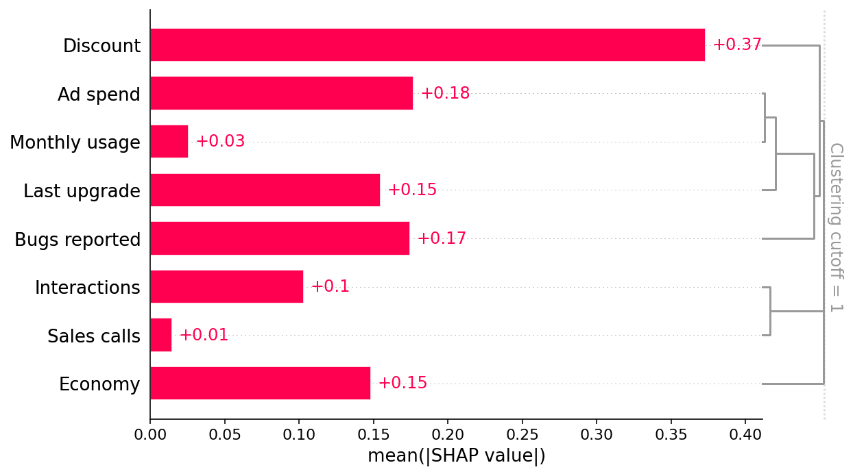
Observed confounding calls for adding controls (Dillon et al - Observed Confounding and Double ML for Ad Spend). Non-confounding redundancy calls for removing them. The trouble is that both look identical in the SHAP redundancy dendrogram. Sales calls and Interactions merge at the very bottom (correlation 0.94 in the DGP).

Main Content

Definition: Non-confounding redundancy (raw line 457)

“The second scenario where causal inference can help is non-confounding redundancy. This occurs when the feature we want causal effects for causally drives, or is driven by, another feature included in the model, but that other feature is not a confounder of our feature of interest.”

Two sub-cases (vault labels):

• Downstream (mediator): $X\to Z\to Y$, with $Z$ in the model. Here $Z$ = Interactions, $X$ = Sales calls.
• Upstream (pure cause of $X$): $Z\to X\to Y$, where $Z$ has no other path to $Y$. Like a confounder it points into $X$, but because it does not reach $Y$ except through $X$ it opens no back-door path.

Cell [10] (raw lines 464-465), verbatim:

# Interactions and sales calls are very redundant with one another.
shap.plots.bar(shap_values, clustering=clust, clustering_cutoff=1)

Fig. 8 is the same bar plot; Sales calls and Interactions merge low in the dendrogram.

Result: Credit splitting between a feature and its mediator (raw line 470)

“Sales Calls directly impact retention, but also have an indirect effect on retention through Interactions. When we include both the Interactions and Sales Calls features in the model the causal effect shared by both features is forced to spread out between them. We can see this in the SHAP scatter plots above, which show how XGBoost underestimates the true causal effect of Sales Calls because most of that effect got put onto the Interactions feature.”

Why most of the effect goes to Interactions (vault gloss). In the DGP the logit weight on Interactions ($0.105$) is three times the direct weight on Sales calls ($0.035$), and $I=S+\text{noise}$. Conditional on $I$, the extra information in $S$ is small. A regularized model fitted on both therefore puts most of the shared signal on $I$.

Result: Effect of each adjustment choice on DML (raw line 472)

“Non-confounding redundancy can be fixed in principle by removing the redundant variables from the model (see below). For example, if we removed Interactions from the model then we will capture the full effect of making a sales call on renewal probability. This removal is also important for double ML, since double ML will fail to capture indirect causal effects if you control for downstream features caused by the feature of interest. In this case double ML will only measure the ‘direct’ effect that does not pass through the other feature. Double ML is however robust to controlling for upstream non-confounding redundancy (where the redundant feature causes the feature of interest), though this will reduce your statistical power to detect true effects.”

Control set includes…	Estimand recovered	Cost
a confounder (needed)	total effect, unbiased	—
a downstream mediator	direct effect only (controlled direct effect)	indirect paths are lost
an upstream pure cause of $X$	total effect, unbiased	less residual variation in $X$, so lower power

The control-or-drop rule under graph uncertainty

Rule: When unsure, control (raw line 474)

“Unfortunately, we often don’t know the true causal graph so it can be hard to know when another feature is redundant with our feature of interest because of observed confounding vs. non-confounding redundancy. If it is because of confounding then we should control for that feature using a method like double ML, whereas if it is a downstream consequence then we should drop the feature from our model if we want full causal effects rather than only direct effects. Controlling for a feature we shouldn’t tends to hide or split up causal effects, while failing to control for a feature we should have controlled for tends to infer causal effects that do not exist. This generally makes controlling for a feature the safer option when you are uncertain.”

Logic. The rule rests on an asymmetry of errors. Over-controlling a mediator biases the estimate toward zero, which is conservative. Under-controlling a confounder can manufacture an effect, as with Ad spend.

Caveat (vault). The asymmetry is not guaranteed. Controlling for a collider or a descendant of a collider can also create spurious effects, and over-controlling a mediator can flip signs when direct and indirect effects have opposite signs. See DAGs and Causal Identification and Table 2 Fallacy.

Demonstration: drop the mediator (cell [11], Fig. 9)

Cell [11] (raw lines 481-489), verbatim:

# Fit, explain, and plot a univariate model with just Sales calls
# Note how this model does not have to split of credit between Sales calls and
# Interactions, so we get a better agreement with the true causal effect.
sales_calls_model = fit_xgboost(X[["Sales calls"]], y)
sales_calls_shap_values = shap.Explainer(sales_calls_model)(X[["Sales calls"]])
shap.plots.scatter(
    sales_calls_shap_values,
    overlay={"True causal effects": marginal_effects(generator, 10000, ["Sales calls"])},
)

Fig. 9: SHAP scatter for the univariate Sales-calls model with the true-effect overlay. The code comment: “this model does not have to split of [sic] credit between Sales calls and Interactions, so we get a better agreement with the true causal effect.”

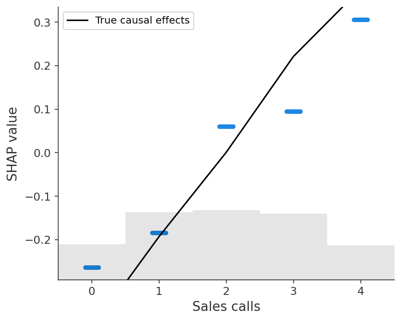
Fig. 9 read off the hosted image, cross-checked against the vault's true-effect computation (not stated in the source text)

The rendered figure (shap.readthedocs.io “latest” build, retrieved 2026-10-13) shows five horizontal SHAP bands, one per value of Sales calls, with the black true-effect line. The y-axis is clipped to about −0.29 to +0.33, so the black line runs off the plot at both ends.

Sales calls	SHAP (univariate model)	True effect (black line, centred logit)
0	about −0.26	below the axis; about −0.4 in Fig. 4
1	about −0.18	about −0.19
2	about +0.06	about 0.00
3	about +0.095	about +0.22
4	about +0.305	above the axis; about +0.38 in Fig. 4

Reading. The SHAP values now rise monotonically, with a 0 → 4 spread of about $0.57$ logits. In the full model (Fig. 4) the Sales-calls panel spreads only about $0.06$, so the univariate fit recovers roughly ten times more of the effect. It still falls short of the true total effect. The black line spans about $0.78$, which matches the vault’s own computation of +0.78 on the logit scale for p5 → p95 = 0 → 4 calls (^ex-true-effects). The SHAP spread is therefore about 73% of the truth. The SHAP steps are also uneven: the 1 → 2 step is large and the 2 → 3 step is small, while the true line is close to linear. “Better agreement”, as the code comment puts it, is accurate. “Recovers the effect” would overstate it.

Likely reasons for the remaining gap (vault interpretation, not tested here). (i) The heavily regularized fit ($\eta =0.001$, depth 2, early stopping after 20 non-improving rounds) shrinks the per-value means towards the overall mean. (ii) The two curves are centred differently: SHAP values average to zero over the data distribution, while marginal_effects centres on the unweighted mean of its grid points. Centring shifts the curves but leaves their spreads unchanged, so (i) is the more likely cause of the shortfall.

Why the univariate model is causal here. Sales calls is a root node of the DAG ($S=[U(0,4)]$). It has no parents, so it has no back-door paths, and $\mathbb{E}[R\mid S]=\mathbb{E}[R\mid do(S)]$. The univariate regression therefore targets the total effect, including the paths $S\to N\to \dots$ through latent Product need. Dropping features gives a causal answer only because $S$ is effectively randomized.

Examples

Example: vault replication — controlling for the mediator (not in the source)

Setup. Linear partialling-out, as in ^ex-replication, with Sales calls as the treatment and all seven other observed features (including Interactions) as controls.

Result. The partialled-out slope is $0.005$ (se $0.010$, $z=0.50$). The true total effect on the probability scale is about $0.041$ per call (p5 → p95), and the naive univariate OLS slope is $0.035$.

Interpretation. Controlling for Interactions, together with Discount, Monthly usage, Bugs reported and Ad spend, all of which are also descendants of Sales calls through Product need, reduces the estimate to roughly the small direct effect ($7\times 0.005=0.035$ on the logit scale, about $0.007$ in probability). The univariate model recovers most of the total.

Example: marketing analogue

TV advertising raises branded search queries, and branded search clicks precede conversions. Branded search spend is then a mediator of TV. Putting both in a driver model, or controlling for search in a DML for TV, credits search with TV’s indirect effect. The estimand choice (total vs direct) must come first. See Blake Nosko Tadelis 2015 - Paid Search Effectiveness - Overview for evidence that branded-search attribution can be largely non-incremental.

Connections

• Causal Estimands — total vs controlled direct effect.
• Spurious Association and Confounds — post-treatment bias in the Bayesian regression treatment.
• Omitted Variables Bias — the regression algebra of including or excluding $Z$.

See Also

• Dillon et al - SHAP and Causal Insights - Overview
• Dillon et al - Unobserved Confounding and Quasi-Experimental Remedies — the case where no choice of controls works.