Dillon et al - Observed Confounding and Double ML for Ad Spend

Summary

Ad spend has zero causal effect on renewal, yet XGBoost ranks it a top-3 driver. Its two causes, Monthly usage and Last upgrade, both drive renewal, and a regularized learner prefers one summary feature to three causal ones. This is observed confounding: every confounder is measured. So the authors apply double/debiased machine learning with econML’s LinearDML. It residualizes treatment and outcome on the controls and regresses residual on residual. The method “correctly identif[ies] that there is no evidence for a causal effect of ad spending on renewal (P-value = 0.85)“. The caveat is that DML works only if all confounders are measured and identified. Without a graph, the SHAP redundancy dendrogram suggests candidate controls.

Overview

“In most real-world datasets features are not independent and unconfounded, so standard predictive models will not learn the true causal effects. As a result, explaining them with SHAP will not reveal causal effects. But all is not lost, sometimes we can fix or at least minimize this problem using the tools of observational causal inference” (raw line 319). Observed confounding is the first of two scenarios where this works. The second is Dillon et al - Non-Confounding Redundancy and the Control-or-Drop Rule.

Main Content

Definition and diagnosis

Definition: Confounded feature; observed confounder (raw line 323)

“A feature is ‘confounded’ when there is another feature that causally affects both the original feature and the outcome we are predicting. If we can measure that other feature it is called an observed confounder.”

In DAG terms: $Z$ confounds $X\to Y$ if $Z$ opens a back-door path $X\leftarrow Z\to Y$. It is an observed confounder if $Z$ is among the available columns.

Cell [8] (raw lines 330-331), verbatim:

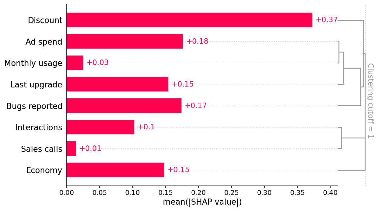
# Ad spend is very redundant with Monthly usage and Last upgrade.
shap.plots.bar(shap_values, clustering=clust, clustering_cutoff=1)

Fig. 6 is the same bar plot; in its dendrogram Ad spend merges low with Monthly usage and Last upgrade.

The “Observed confounding” paragraph opens with the example itself: “An example of this in our scenario is the Ad Spend feature. Even though Ad Spend has no direct causal effect on retention, it is correlated with the Last Upgrade and Monthly Usage features, which do drive retention.” (raw line 336). It then gives the mechanism:

Mechanism: Regularization selects the redundant summary feature (raw line 336)

“Our predictive model identifies Ad Spend as the one of the best single predictors of retention because it captures so many of the true causal drivers through correlations. XGBoost imposes regularization, which is a fancy way of saying that it tries to choose the simplest possible model that still predicts well. If it could predict equally well using one feature rather than three, it will tend to do that to avoid overfitting. But this means that if Ad Spend is highly correlated with both Last Upgrade and Monthly Usage, XGBoost may use Ad Spend instead of the causal features! This property of XGBoost (or any other machine learning model with regularization) is very useful for generating robust predictions of future retention, but not good for understanding which features we should manipulate if we want to increase retention.”

In the DGP, $A=M\cdot U(0.9,0.99)+1[L<1]+1[L<2]$. One split on $A$ captures part of the steep recent-upgrade effect, through $L<1$ and $L<2$, and the usage effect, through $M$.

Why this failure is the dangerous one (raw line 338)

“Unlike the bug reporting example, there is nothing intuitively wrong with the conclusion that increasing ad spend increases retention. Without proper attention to what our predictive model is, and is not, measuring, we could easily have proceeded with this finding and only learned our mistake after increasing spending on advertising and not getting the renewal results we expected.”

The paragraph opens: “This highlights the importance of matching the right modeling tools to each question.” A face-validity review would pass it. Wrong signs at least draw attention; plausible signs do not.

The remedy: double/debiased ML

“The good news for Ad Spend is that we can measure all the features that could confound it (those features with arrows into Ad Spend in our causal graph above). Therefore, this is an example of observed confounding, and we should be able to disentangle the correlation patterns using only the data we’ve already collected; we just need to use the right tools from observational causal inference. These tools allow us to specify what features could confound Ad Spend and then adjust for those features, to get an unconfounded estimate” (line 342). Double ML “uses any machine learning model you want to first deconfound the feature of interest (i.e. Ad Spend) and then estimate the average causal effect of changing that feature (i.e. the average slope of the causal effect)” (line 344).

Algorithm: Double ML as stated in the article (raw lines 346-350)

1. “Train a model to predict a feature of interest (i.e. Ad Spend) using a set of possible confounders (i.e. any features not caused by Ad Spend).”
2. “Train a model to predict the outcome (i.e. Did Renew) using the same set of possible confounders.”
3. “Train a model to predict the residual variation of the outcome (the variation left after subtracting our prediction) using the residual variation of the causal feature of interest.”

Formal version (vault gloss). This is the partially linear model of Regularization Bias and the Partially Linear Model:

$$Y=\theta T+g(W)+\epsilon ,\mathbb{E}[\epsilon \mid T,W]=0;T=m(W)+V,\mathbb{E}[V\mid W]=0,$$

with $Y$ = Did renew, $T$ = Ad spend and $W$ = controls. Estimate $\ell (W)=\mathbb{E}[Y\mid W]$ and $m(W)$ with ML, form residuals $\tilde{Y}=Y-\hat{\ell }(W)$ and $\tilde{T}=T-\hat{m}(W)$ (cross-fitted, Cross-Fitting and Sample Splitting), and set

$$\hat{\theta }=\frac{{\sum }_i{\tilde{T}}_i{\tilde{Y}}_i}{{\sum }_i{\tilde{T}}_i^2}.$$

The score is Neyman-orthogonal, so first-order errors in $\hat{\ell },\hat{m}$ do not bias $\hat{\theta }$. This yields $\sqrt{n}$-normal inference, which is the source of the p-value. Identification requires conditional ignorability $T\perp \{Y(t){\}}_t\mid W$ (Conditional Independence Assumption) and overlap, meaning $V$ has non-degenerate variance.

The article’s intuition (line 352): “if Ad Spend causes renewal, then the part of Ad Spend that can’t be predicted by other confounding features should be correlated with the part of renewal that can’t be predicted by other confounding features. Stated another way, double ML assumes that there is an independent (unobserved) noise feature that impacts Ad Spend (since Ad Spend is not perfectly determined by the other features), so we can impute the value of this independent noise feature and then train a model on this independent feature to predict the output.” Here that noise feature is the $U(0.9,0.99)$ multiplier.

Implementation (cell [9], Fig. 7)

“While we could do all the double ML steps manually, it is easier to use a causal inference package like econML or CausalML. Here we use econML’s LinearDML model. This returns a P-value of whether that treatment has a non-zero a [sic] causal effect” (line 354).

Cell [9] (raw lines 361-448), verbatim:

import matplotlib.pyplot as plt
from econml.dml import LinearDML
from sklearn.base import BaseEstimator, clone
 
class RegressionWrapper(BaseEstimator):
    """Turns a classifier into a 'regressor'.
 
    We use the regression formulation of double ML, so we need to approximate the classifer
    as a regression model. This treats the probabilities as just quantitative value targets
    for least squares regression, but it turns out to be a reasonable approximation.
    """
 
    def __init__(self, clf):
        self.clf = clf
 
    def fit(self, X, y, **kwargs):
        self.clf_ = clone(self.clf)
        self.clf_.fit(X, y, **kwargs)
        return self
 
    def predict(self, X):
        return self.clf_.predict_proba(X)[:, 1]
 
# Run Double ML, controlling for all the other features
def double_ml(y, causal_feature, control_features):
    """Use doubleML from econML to estimate the slope of the causal effect of a feature."""
    xgb_model = xgboost.XGBClassifier(objective="binary:logistic", random_state=42)
    est = LinearDML(model_y=RegressionWrapper(xgb_model))
    est.fit(y, causal_feature, W=control_features)
    return est.effect_inference()
 
def plot_effect(effect, xs, true_ys, ylim=None):
    """Plot a double ML effect estimate from econML as a line.
 
    Note that the effect estimate from double ML is an average effect *slope* not a full
    function. So we arbitrarily draw the slope of the line as passing through the origin.
    """
    plt.figure(figsize=(5, 3))
 
    pred_xs = [xs.min(), xs.max()]
    mid = (xs.min() + xs.max()) / 2
    [effect.pred[0] * (xs.min() - mid), effect.pred[0] * (xs.max() - mid)]
 
    plt.plot(xs, true_ys - true_ys[0], label="True causal effect", color="black", linewidth=3)
    point_pred = effect.point_estimate * pred_xs
    pred_stderr = effect.stderr * np.abs(pred_xs)
    plt.plot(
        pred_xs,
        point_pred - point_pred[0],
        label="Double ML slope",
        color=shap.plots.colors.blue_rgb,
        linewidth=3,
    )
    # 99.9% CI
    plt.fill_between(
        pred_xs,
        point_pred - point_pred[0] - 3.291 * pred_stderr,
        point_pred - point_pred[0] + 3.291 * pred_stderr,
        alpha=0.2,
        color=shap.plots.colors.blue_rgb,
    )
    plt.legend()
    plt.xlabel("Ad spend", fontsize=13)
    plt.ylabel("Zero centered effect")
    if ylim is not None:
        plt.ylim(*ylim)
    plt.gca().xaxis.set_ticks_position("bottom")
    plt.gca().yaxis.set_ticks_position("left")
    plt.gca().spines["right"].set_visible(False)
    plt.gca().spines["top"].set_visible(False)
    plt.show()
 
# estimate the causal effect of Ad spend controlling for all the other features
causal_feature = "Ad spend"
control_features = [
    "Sales calls",
    "Interactions",
    "Economy",
    "Last upgrade",
    "Discount",
    "Monthly usage",
    "Bugs reported",
]
effect = double_ml(y, X[causal_feature], X.loc[:, control_features])
 
# plot the estimated slope against the true effect
xs, true_ys = marginal_effects(generator, 10000, X[["Ad spend"]], logit=False)[0]
plot_effect(effect, xs, true_ys, ylim=(-0.2, 0.2))

Code walk-through.

Component	What it does	Notes
RegressionWrapper	wraps an sklearn classifier so that predict returns predict_proba(X)[:, 1]	the docstring explains that the regression formulation of DML “treats the probabilities as just quantitative value targets for least squares regression, but it turns out to be a reasonable approximation” — the outcome is binary but modeled on the probability scale
double_ml	LinearDML(model_y=RegressionWrapper(XGBClassifier(...))), fit(y, T, W=controls), returns effect_inference()	only model_y is set; the treatment model is left at econML’s default. No X (effect modifiers) is passed, so $\theta$ is a single constant slope
plot_effect	draws the true effect (anchored at the left end) and the DML line $\hat{\theta }x$ re-anchored to 0 at $x_{\min }$, with a band of $\pm 3.291 \cdot \text{se} \cdot	x
controls	Sales calls, Interactions, Economy, Last upgrade, Discount, Monthly usage, Bugs reported	i.e. all seven other observed features
truth	marginal_effects(generator, 10000, X[["Ad spend"]], logit=False)[0]	probability scale, to match DML’s regression on probabilities; iterating a one-column DataFrame yields its name

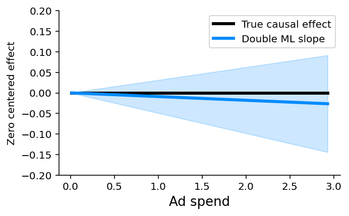
Fig. 7: the “Double ML slope” line with its shaded 99.9% band against the flat black “True causal effect” line, $y$-limits $(-0.2,0.2)$, $x$-axis “Ad spend”. Result in the text: the method “works beautifully in our scenario, correctly identifying that there is no evidence for a causal effect of ad spending on renewal (P-value = 0.85)“.

Reading of Fig. 7 (vault reading of the plotted image, approximate; not stated in the text)

Quantity	Value read from the plot
$x$-range (Ad spend)	about 0 to 2.93
True causal effect	flat at 0 across the whole range
DML line at right end ($x\approx 2.93$)	about $-0.026$, so $\hat{\theta }\approx -0.009$ per unit of Ad spend
99.9% band at right end	about $-0.145$ to $+0.09$ (half-width $\approx 0.118$)
Implied band on the slope	$\hat{\theta }\pm 3.291\text{se}\approx -0.009\pm 0.040$, so $\text{se}\approx 0.012$

The band fans out symmetrically from the origin and comfortably covers the true line at 0. The implied $z\approx -0.009/0.012\approx -0.7$ ($p\approx 0.5$) is not significant, matching the text’s conclusion. It does not match the stated $p=0.85$ exactly ($|z|\approx 0.19$). The rendered image may come from a different execution of the notebook than the one the text quotes (XGBoost subsample=0.5 is random), or the reading may be off. Treat the slope figures as order-of-magnitude.

Assumptions and choosing controls

Proviso: DML needs every confounder measured (raw line 453)

“Remember, double ML (or any other observational causal inference method) only works when you can measure and identify all the possible confounders of the feature for which you want to estimate causal effects. Here we know the causal graph and can see that Monthly Usage and Last Upgrade are the two direct confounders we need to control for. But if we didn’t know the causal graph we could still look at the redundancy in the SHAP bar plot and see that Monthly Usage and Last Upgrade are the most redundant features and so are good candidates to control for (as are Discounts and Bugs Reported).”

The heuristic “control for what SHAP clusters with the treatment” is only a candidate generator. Redundancy can come from confounders, which should be controlled, from mediators, which should not (Dillon et al - Non-Confounding Redundancy and the Control-or-Drop Rule), or from colliders, which should not be controlled either. The source does not discuss colliders. See DAGs and Causal Identification and Table 2 Fallacy.

Examples

Example: vault replication with linear nuisance models (not in the source)

Setup. Same generator with seed 0 and $n=10,000$. Replace the XGBoost nuisances by OLS. For Last upgrade, add the features $1[L<1]$, $1[L<2]$ and $1/(L/4+0.25)$. There is no cross-fitting and the standard errors are heteroskedasticity-robust. Outcome: the binary renewal on the probability scale.

Treatment	Naive OLS slope	Partialled-out slope (se)	True slope, p5 → p95 (probability scale)
Ad spend	+0.183	−0.358 (0.310), $z=-1.16$	0
Discount	−1.289	−1.078 (0.048), $z=-22.5$	+0.064

Interpretation. For Ad spend, partialling out removes the spurious positive slope. The estimate is no longer distinguishable from zero, which matches the source’s qualitative result ($p=0.85$ with XGBoost nuisances). The standard error is large because Ad spend is nearly deterministic given $(M,L)$: the residual variation comes only from the $U(0.9,0.99)$ multiplier, a thin overlap. Discount stays strongly negative even with all observed controls, which previews Dillon et al - Unobserved Confounding and Quasi-Experimental Remedies.

Example: minimal call pattern

from econml.dml import LinearDML
est = LinearDML(model_y=RegressionWrapper(xgboost.XGBClassifier(objective="binary:logistic", random_state=42)))
est.fit(y, X["Ad spend"], W=X[["Sales calls", "Interactions", "Economy", "Last upgrade",
                               "Discount", "Monthly usage", "Bugs reported"]])
inf = est.effect_inference()   # point_estimate, stderr, p-value

This is condensed from cell [9]; the full code is above.

Connections

• Causal Machine Learning - Overview, DML Estimators for ATE and the Interactive Model — the general DML family. LinearDML is the partially-linear case.
• R-Learner and Orthogonal CATE Estimation, Honest Trees and Causal Forests — the heterogeneous-effect extension: pass X to obtain $\theta (X)$.
• Nuisance Parameter Bias Simulation and Logic of Regression Adjustment — regression adjustment and the role of nuisance fits.
• Experimental Benchmarks for Observational Ad Measurement — in real ad data, DML with more than 5,000 features still overstated lift. The “all confounders observed” assumption is the binding one.
• Fisher Rudin Dominici 2019 - Model Class Reliance - Overview — Ad spend vs its parents is a textbook Rashomon pair.

See Also

• Dillon et al - SHAP and Causal Insights - Overview
• ^def-redundancy-clustering — how to read the dendrogram used to pick controls.