Dillon et al - SHAP Plots vs True Causal Effects

Summary

The empirical core of the notebook. The global SHAP bar plot ranks Discount, Ad spend and Bugs reported as the top three renewal drivers, which “at first glance looks reasonable”. Overlaying the true interventional effect curve (computed with the DGP’s do-operator) on each SHAP scatter plot exposes two problems. (1) Unobserved confounding by Product need gives Bugs reported a positive SHAP slope although its effect is zero, and Discount a negative slope although its effect is positive. (2) Observed confounding / statistical redundancy gives Ad spend a positive SHAP slope although “the black line is flat”. Economy’s SHAP curve tracks the truth.

Overview

SHAP values for a tree ensemble decompose each prediction $f(x)$ additively: $f(x)={\varphi }_0+{\sum }_j{\varphi }_j(x)$. The bar plot shows $\frac{1}{n}{\sum }_i|{\varphi }_j(x_i)|$, and the scatter plot shows ${\varphi }_j(x_i)$ against $x_{ij}$. Formal definitions are owned by Kumar et al 2020 - Problems with Shapley-Value Explanations - Overview. shap.Explainer(model) on an XGBoost booster uses the tree explainer. With objective="reg:logistic", SHAP values are in the model’s log-odds (margin) units, which is why the true-effect overlay in cell [6] is put on the logit scale (logit=True).

Main Content

Step 1 — global importance with redundancy clustering (cell [3], Fig. 1)

Cell [3] (raw lines 144-150), verbatim:

import shap
 
explainer = shap.Explainer(model)
shap_values = explainer(X)
 
clust = shap.utils.hclust(X, y, linkage="single")
shap.plots.bar(shap_values, clustering=clust, clustering_cutoff=1)

Fig. 1: a horizontal bar chart of mean |SHAP| per feature, with a dendrogram on the right built by shap.utils.hclust(X, y, linkage="single") and cut at clustering_cutoff=1. The text: “the discount offered, ad spend, and number of bugs reported are the top three factors driving the model’s prediction of customer retention. This is interesting and at first glance looks reasonable. The bar plot also includes a feature redundancy clustering which we will use later” (raw line 155). How to read the dendrogram is covered in Dillon et al - When SHAP Recovers Causal Effects.

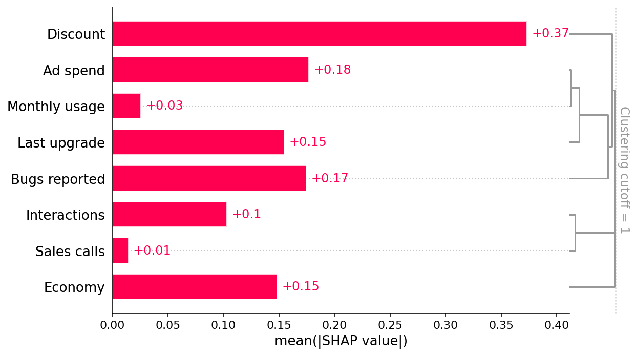
Fig. 1 read bar by bar (vault reading of the hosted image, not stated in the source text)

The source text names only the top three features. The rendered figure (shap.readthedocs.io “latest” build, image retrieved 2026-10-13; values can shift slightly between documentation builds) prints these mean |SHAP| labels, in log-odds units:

| Rank | Feature | mean |SHAP| | True total effect, p5 → p95 (^ex-true-effects) | |---|---|---|---| | 1 | Discount | 0.37 | +0.09 (small positive) | | 2 | Ad spend | 0.18 | 0 | | 3 | Bugs reported | 0.17 | 0 | | 4= | Last upgrade | 0.15 | −0.92 (convex) | | 4= | Economy | 0.15 | +0.50 | | 6 | Interactions | 0.10 | +0.31 | | 7 | Monthly usage | 0.03 | +0.24 | | 8 | Sales calls | 0.01 | +0.78 |

The plot draws the bars in dendrogram order, not rank order: Discount, Ad spend, Monthly usage, Last upgrade, Bugs reported, Interactions, Sales calls, Economy. In the dendrogram, Ad spend and Monthly usage merge first, then Last upgrade joins them, then Bugs reported, then Discount. Interactions and Sales calls form a separate tight pair. Economy joins only at the root. The ranking is close to inverted relative to the truth. The three features with zero or near-zero causal effect hold the top three places, and the feature with the largest total effect, Sales calls, comes last.

Step 2 — dependence (scatter) plots (cell [4], Fig. 2)

Cell [4] (raw lines 164-164), verbatim:

shap.plots.scatter(shap_values, ylabel="SHAP value\n(higher means more likely to renew)")

Fig. 2: one scatter panel per feature. “SHAP scatter plots show how changing the value of a feature impacts the model’s prediction of renewal probabilities. If the blue dots follow an increasing pattern, this means that the larger the feature, the higher is the model’s predicted renewal probability” (line 157). The surprising patterns (bugs reported increasing, discount decreasing) set up Dillon et al - Prediction Tasks vs Causal Tasks.

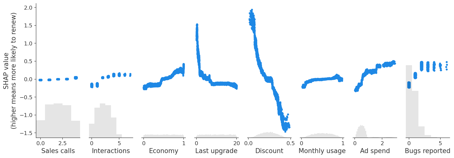
Fig. 2 read panel by panel (vault reading of the hosted image, not stated in the source text)

The panels share one y-axis (SHAP value, log-odds, about −1.5 to +2.0). Each panel also shows a grey histogram of the feature’s distribution. Panels from left to right:

Panel	x range	SHAP pattern
Sales calls	0-4 (integers)	almost flat: five tight bands from about −0.02 to +0.04
Interactions	0-7	rising step bands from about −0.2 at 0-1 to about +0.15 at 4-5, then flat where data are sparse
Economy	0-1	steady rise from about −0.25 to +0.3, with a step near 0.5
Last upgrade	0-20 months	steep convex fall from about +1.5 at 0 to about −0.15 by month 5, then flat near −0.15 to −0.2
Discount	0-0.5	the largest spread in the figure: falls monotonically from about +1.8 at 0 to about −1.4 at 0.45
Monthly usage	0-1	gentle rise from about −0.2 to 0, then flat; a small range
Ad spend	0-2.7	stepped rise from about −0.3 to +0.45; most mass sits at 0.2-1
Bugs reported	0-6 (integers)	about −0.15 at 0, about +0.1 at 1 and +0.3 to +0.5 at 2 or more

Careful wording

The source’s phrase “how changing the value of a feature impacts the model’s prediction” is accurate only about the model: it describes how $f$ responds. The article’s whole point is that this is not how the outcome responds. See Janzing et al 2020 - Feature Relevance as a Causal Problem - Overview for the system-vs-world distinction.

Step 3 — ground-truth overlay (cell [6], Fig. 4)

Algorithm: marginal_effects — true interventional effect curves (cell [6], raw lines 254-273)

Inputs: a generative model $g$ (here generator), num_samples $m$, columns, max_points $K=20$, logit, seed.

1. Draw one observational sample $X\sim g(m)$ (default seed 0).
2. For each column $c$, build a grid ${\mathcal{G}}_c$ from the unique values of the nearest-rank percentiles at $K$ evenly spaced levels $0,\dots ,100$. Discrete features such as Bugs reported give fewer than $K$ points.
3. For each $x\in {\mathcal{G}}_c$: simulate $X^{(x)}\sim g(m,\text{fixed}=\{c:x\})$ with the same seed (a do-intervention; see ^def-fixable-dataframe) and record $v(x)={\overline{R}}^{(x)}$, the mean of the binary renewals. If logit, use $\mathrm{logit}v(x)$ instead.
4. Centre: $\tilde{v}(x)=v(x)-\frac{1}{|{\mathcal{G}}_c|}{\sum }_{x^{\prime }}v(x^{\prime })$, so the curve is comparable to SHAP values, which also have mean roughly 0.
5. Return a list of $({\mathcal{G}}_c,\tilde{v})$ pairs, one per column.

The estimand is $\mathrm{logit}\mathrm{Pr}(R=1\mid do(X_c=x))$, centred. It is a total causal effect: everything downstream of $c$ responds.

Cell [6] (raw lines 254-279), verbatim:

def marginal_effects(generative_model, num_samples=100, columns=None, max_points=20, logit=True, seed=0):
    """Helper function to compute the true marginal causal effects."""
    X = generative_model(num_samples)
    if columns is None:
        columns = X.columns
    ys = [[] for _ in columns]
    xs = [X[c].values for c in columns]
    xs = np.sort(xs, axis=1)
    xs = [xs[i] for i in range(len(xs))]
    for i, c in enumerate(columns):
        xs[i] = np.unique([np.nanpercentile(xs[i], v, method="nearest") for v in np.linspace(0, 100, max_points)])
        for x in xs[i]:
            Xnew = generative_model(num_samples, fixed={c: x}, seed=seed)
            val = Xnew["Did renew"].mean()
            if logit:
                val = scipy.special.logit(val)
            ys[i].append(val)
        ys[i] = np.array(ys[i])
    ys = [ys[i] - ys[i].mean() for i in range(len(ys))]
    return list(zip(xs, ys))
 
shap.plots.scatter(
    shap_values,
    ylabel="SHAP value\n(higher means more likely to renew)",
    overlay={"True causal effects": marginal_effects(generator, 10000, X.columns)},
)

Fig. 4: the SHAP scatter panels from Fig. 2 with a black “True causal effects” line overlaid on each.

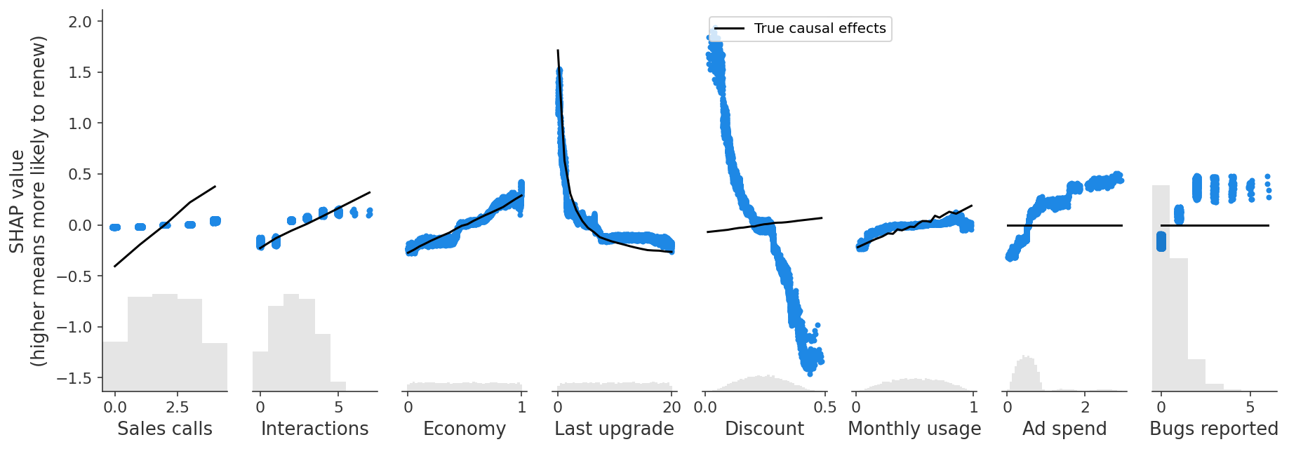
Diagnoses read off Fig. 4

Finding 1: Unobserved confounding flips Bugs reported (raw lines 247, 284)

“There are lots of relationships in this graph, but the first important concern is that some of the features we can measure are influenced by unmeasured confounding features like product need and bugs faced. For example, users who report more bugs are encountering more bugs because they use the product more, and they are also more likely to report those bugs because they need the product more. Product need has its own direct causal effect on renewal.” Hence “the correlation we end up capturing in predictive models between bugs reported and renewal combines a small negative direct effect of bugs faced and a large positive confounding effect from product need.”

Result: “The predictive model captures an overall positive effect of bugs reported on retention (as shown with SHAP), even though the causal effect of reporting a bug is zero, and the effect of encoutering [sic] a bug is negative.”

Graph explanation. The back-door path is Bugs reported ← Product need → Did renew, plus Bugs reported ← Bugs faced ← Monthly usage ← Product need. Neither Product need nor Bugs faced is observed, so the path cannot be closed.

Finding 2: Unobserved confounding flips Discount (raw line 286)

Discounts “are also driven by unobserved customer need for the product. Our predictive model finds a negative relationship between discounts and retention, driven by this correlation with the unobserved feature, Product Need, even though there is actually a small positive causal effect of discounts on renewal!” The ceteris-paribus reading: “if two customers with [sic] have the same Product Need and are otherwise similar, then the customer with the larger discount is more likely to renew.”

Mechanism. $D$ decreases in $\sigma (N)$, and $N$ enters $\mathrm{logit}p$ with weight $1.26$ against $0.35$ for $D$. The confounding path Discount ← Product need → Did renew dominates.

Finding 3: Observed confounding / redundancy inflates Ad spend (raw lines 288-290)

“Ad Spend has a similar problem - it has no causal effect on retention (the black line is flat), but the predictive model is picking up a positive effect!” The next paragraph, quoted whole: “In this case, Ad Spend is only driven by Last Upgrade and Monthly Usage, so we don’t have an unobserved confounding problem, instead we have an observed confounding problem. There is statistical redundancy between Ad Spend and features that influence Ad Spend. When we have the same information captured by several features, predictive models can use any of those features for prediction, even though they are not all causal. While Ad Spend has no causal effect on renewal itself, it is strongly correlated with several features that do drive renewal. Our regularized model identifies Ad Spend as a useful predictor because it summarizes multiple causal drivers (so leading to a sparser model), but that becomes seriously misleading if we start to interpret it as a causal effect.” (raw line 290, complete)

The authors call this “a second, sneakier problem”. Unlike the bug sign, nothing about it looks wrong. The full treatment and fix are in Dillon et al - Observed Confounding and Double ML for Ad Spend.

Roadmap stated by the source (raw line 292)

“We will now tackle each piece of our example in turn to illustrate when predictive models can accurately measure causal effects, and when they cannot. We will also introduce some causal tools that can sometimes estimate causal effects in cases where predictive models fail.” The four following notes take the cases in order: Economy, Ad spend, Sales calls, then Discount and Bugs reported.

Examples

Example: reading the overlay for each feature (all eight panels of Fig. 4)

Fig. 4 is Fig. 2 with a black “True causal effects” line added to each panel. The first five rows follow the source text. The rows marked † are the vault’s reading of the hosted image (retrieved 2026-10-13); the source text does not discuss those panels.

Feature	SHAP pattern (Fig. 4)	True effect (black line)	Agreement	Gap explained by
Economy	rises from about −0.25 to +0.3	rises from about −0.27 to +0.3	close match	— (independent)
Bugs reported	rises from −0.15 to about +0.4	flat at 0	wrong sign	unobserved Product need, Bugs faced
Discount	falls from about +1.8 to −1.4	rises slightly, from about −0.07 to +0.07	wrong sign, magnitude about 20 times too large	unobserved Product need
Ad spend	stepped rise from −0.3 to +0.45	flat at 0	spurious effect	observed confounders Monthly usage and Last upgrade (redundancy)
Sales calls	almost flat (about −0.02 to +0.04)	rises from about −0.4 to +0.38	severe underestimate	credit split with Interactions (Dillon et al - Non-Confounding Redundancy and the Control-or-Drop Rule)
Interactions †	rises from about −0.2 to +0.15 over 0-5	rises from about −0.22 to +0.32 over 0-7	roughly tracks over 0-4; flatter at the sparse top end	Interactions is a mediator of Sales calls with a direct effect of its own, so its own SHAP is not badly biased. The problem shows up on Sales calls
Last upgrade †	convex fall from about +1.5 to −0.2	convex fall from about +1.7 to −0.25	close match, including the curvature of $0.7/(L/4+0.25)$	Last upgrade is a root node; its link to Ad spend is a fork through it, not a confounder of it
Monthly usage †	rises from about −0.2 to 0, then flat	rises steadily from about −0.2 to +0.19	tracks at low usage, underestimates at high usage	part of its credit goes to Ad spend, which it causes (the same redundancy as Finding 3, seen from the other side)

Numerical true-effect sizes are tabulated in ^ex-true-effects.

Connections

• Hooker Mentch Zhou 2021 - Permute-and-Predict Extrapolation - Overview and Strobl et al 2008 - Conditional Variable Importance - Overview — other importance measures. They also describe the fitted model under correlated features, not causal structure.
• Fisher Rudin Dominici 2019 - Model Class Reliance - Overview — a model relying on Ad spend and one relying on its parents can be equally accurate (Rashomon set). SHAP reports the reliance of the one model that was fitted.
• Spurious Association and Confounds — the same spurious and masked associations in Bayesian regression.
• Omitted Variables Bias — the regression formula for Findings 1-2.

See Also

• Dillon et al - SHAP and Causal Insights - Overview
• Dillon et al - When SHAP Recovers Causal Effects