Dillon et al - Unobserved Confounding and Quasi-Experimental Remedies

Summary

The hardest case. Discount and Bugs reported both depend on the unmeasured Product need (and Bugs faced). They look “fairly independent” of the other measured features in the SHAP dendrogram, so no redundancy diagnostic flags them. Here “both predictive models and causal models that require confounders to be observed, like double ML, will fail”: DML with all seven observed controls returns a large negative Discount effect, while the true effect is small and positive. The only general remedy is randomization: experiments, or partial randomization through instrumental variables (random nudges), difference-in-differences (staggered rollouts) and regression discontinuity (sharp eligibility cut-offs).

Overview

“Double ML (or any other causal inference method that assumes unconfoundedness) only works when you can measure and identify all the possible confounders of the feature for which you want to estimate causal effects. If you can’t measure all the confounders then you are in the hardest possible scenario: unobserved confounding” (raw line 496).

Main Content

Definition: Unobserved confounding (raw lines 496, 510)

A feature suffers unobserved confounding when some common cause of it and the outcome is not measured. Formally, there is a back-door path $X\leftarrow U\to Y$ with $U$ outside the available columns, so no adjustment set built from observed features blocks it, and the conditional-ignorability assumption of selection on observables fails. In the example: “The Discount and Bugs Reported features both suffer from unobserved confounding because not all important variables (e.g., Product Need and Bugs Faced) are measured in the data. Even though both features are relatively independent of all the other features in the model, there are important drivers that are unmeasured.”

Cell [12] (raw lines 503-505), verbatim:

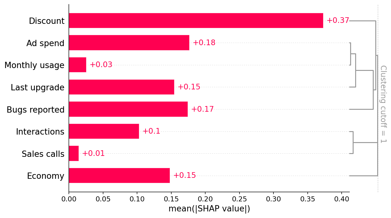
# Discount and Bugs reported seem are fairly independent of the other features we can
# measure, but they are not independent of Product need, which is an unobserved confounder.
shap.plots.bar(shap_values, clustering=clust, clustering_cutoff=1)

Fig. 10 is the same bar plot again. Discount and Bugs reported do not merge low with other features, so the dendrogram looks reassuring and is wrong to be.

, Fig. 11)

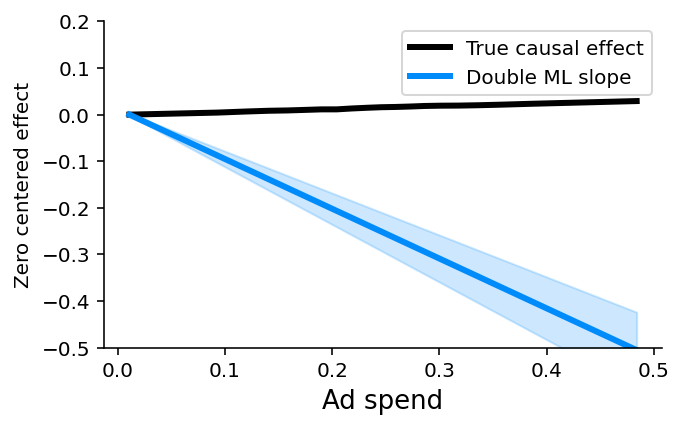
“In this case, both predictive models and causal models that require confounders to be observed, like double ML, will fail. This is why double ML estimates a large negative causal effect for the Discount feature even when controlling for all other observed features.”

Controls used: Sales calls, Interactions, Economy, Last upgrade, Monthly usage, Ad spend, Bugs reported. Two of these, Monthly usage and Bugs reported, are children of Product need and act as partial proxies for it, but they do not block the path Discount ← Product need → Did renew.

Cell [13] (raw lines 517-532), verbatim:

# estimate the causal effect of Ad spend controlling for all the other features
causal_feature = "Discount"
control_features = [
    "Sales calls",
    "Interactions",
    "Economy",
    "Last upgrade",
    "Monthly usage",
    "Ad spend",
    "Bugs reported",
]
effect = double_ml(y, X[causal_feature], X.loc[:, control_features])
 
# plot the estimated slope against the true effect
xs, true_ys = marginal_effects(generator, 10000, X[[causal_feature]], logit=False)[0]
plot_effect(effect, xs, true_ys, ylim=(-0.5, 0.2))

The cell’s first comment says “Ad spend” but the code estimates the effect of Discount, a copy-paste remnant from cell [9]. Fig. 11 shows the DML slope sloping steeply down against a gently rising black true-effect line, with $y$-limits $(-0.5,0.2)$.

Reading of Fig. 11 (vault reading of the plotted image, approximate; not stated in the text)

Quantity	Value read from the plot
$x$-axis label	”Ad spend” (the label is also a cell [9] copy-paste remnant; the plotted range is the Discount range)
$x$-range (Discount)	about 0.01 to 0.485
True causal effect	rises gently from 0 to about $+0.03$ at the right end, a slope of roughly $+0.06$
DML line at right end	reaches the lower $y$-limit $-0.5$ at $x\approx 0.485$, so $\hat{\theta }\approx -1.05$ (probability per unit of Discount)
99.9% band at right end	upper edge about $-0.43$; lower edge clipped below $-0.5$. Half-width $\approx 0.075$. plot_effect draws the band as $\pm 3.291,\text{se},

The whole band lies far below the true line. The estimate is wrong in sign and roughly 17 times the true magnitude, and it is confidently wrong: $z\approx -20$. That is the text’s “large negative” effect.

What can work

Claim: Only (quasi-)randomization identifies effects here (raw line 537)

“Barring the ability to measure the previously unmeasured features (or features correlated with them), finding causal effects in the presence of unobserved confounding is difficult. In these situations, the only way to identify causal effects that can inform policy is to create or exploit some randomization that breaks the correlation between the features of interest and the unmeasured confounders. Randomized experiments remain the gold standard for finding causal effects in this context.”

Note the escape clause “(or features correlated with them)“. Good enough proxies of the confounder can help partially, but in the replication below the observed proxies Monthly usage and Bugs reported are far from sufficient.

Partial-randomization designs named by the source (raw line 539)

“Specialized causal tools based on the principals [sic] of instrumental variables, differences-in-differences, or regression discontinuities can sometimes exploit partial randomization even in cases where a full experiment is impossible.”

Design	Source’s use case	Vault note
Instrumental variables	”we cannot randomly assign a treatment, but we can randomly nudge some customers towards treatment, like sending an email encouraging them to explore a new product feature”	Instrumental Variables
Difference-in-differences	”when the introduction of new treatments is staggered across groups”	Differences-in-Differences
Regression discontinuity	”when patterns of treatment exhibit sharp cut-offs (for example qualification for treatment based on a specific, measurable trait like revenue over $5,000 per month)“	Regression Discontinuity Designs

Examples

Example: vault replication — Discount with all observed controls (not in the source)

Setup. Linear partialling-out, as in ^ex-replication, with the source’s control set.

Estimator	Discount slope (probability per unit discount)
Naive OLS	−1.289
Partialled out on 7 observed controls	−1.078 (se 0.048)
True interventional slope, p5 → p95	+0.064

Interpretation. Adjusting for the observed proxies removes only about a sixth of the bias. The estimate is wrong in sign, very precise and very significant. Precision is no protection against confounding.

Example: designing a randomized discount test

Setup. The retention team wants the effect of discount depth.

Design. Randomize discount levels (say 0%, 10%, 20%) within each salesperson’s renewal book for one cycle, or randomize an eligibility nudge as an instrument if the salespeople must keep discretion. Analyze with an intent-to-treat contrast, then scale by the first stage.

Why. Randomization breaks the Discount ← Product need edge. Product need is then balanced across arms in expectation, and the dendrogram’s blind spot no longer matters.

Example: the advertising version

Ad exposure on a platform is targeted at users with high latent purchase intent. That is the advertising version of “high discounts to customers they think are less likely to be interested”, with the sign reversed. Observational adjustment on rich user features still misstates lift by large factors (Experimental Benchmarks for Observational Ad Measurement). Conversion-lift and geo experiments are the randomized remedy (Conversion Lift Studies on Ad Platforms, Geo-Experiment Methodology - Overview).

Connections

• Sensitivity Analysis in Observational Studies — how strong an unmeasured confounder would need to be to overturn an estimate.
• Q - Uncovering Causal Estimates from Non-Experimental Data — vault Q&A comparing IV, DiD, RD and matching.
• Observational vs Experimental Methods in Advertising and Activity Bias in Advertising — the same failure in ad measurement.
• Blake Nosko Tadelis 2015 - Paid Search Effectiveness - Overview — a field experiment overturning an observational search-ad ROI.

See Also

• Dillon et al - SHAP and Causal Insights - Overview
• ^finding-discount — the SHAP side of the same failure.