When is Multicollinearity an Issue?

A causal perspective

Author

Matthew Reda

Multicollinearity arises when independent variables in a regression model are highly correlated, leading to challenges in estimating individual effects accurately. This issue can inflate standard errors, reduce the precision of coefficient estimates, and complicate the interpretation of results. Understanding when multicollinearity becomes problematic is crucial for developing robust regression models. This section explores the conditions under which multicollinearity affects model performance, discusses its implications, and provides strategies for detection and mitigation.

The DAG

Figure 1: The causal graph reflects our assumptions about the data-generating process in this example. This model may need refinement, so it’s essential to review it with experts and stakeholders to enhance its structure and incorporate additional factors that could influence the variables of interest.

How to read a DAG

A Directed Acyclic Graph (DAG) serves as a model of causality, where directional relationships between nodes indicate that causes flow from one node to another along the arrows, forming a distinct pathway of influence. Each arrow represents a causal link, signaling how changes in one node could potentially impact another. In a DAG, the relationships between nodes (depicted by an arrow) are not restricted to being linear; they can incorporate complex, non-linear interactions.

Edges will be color-coded to emphasize whether they represent causal paths (green ), biasing paths (red ), or non-causal paths (black ). Refer to Figure 2 and Figure 3.

Nodes indicating exposures (factors for which we want to understand the effect) will have a green background (). The outcome variable of interest will have a blue background (), while variables adjusted for will have a light gray background (). Nodes with a dashed outline represent elements that are challenging or impossible to observe directly, while nodes with a solid outline and no fill represent variables for which data is available or can be acquired.

How Effective is Paid Search at Driving Sales?

To accurately measure the impact of Paid Search on Sales, we must carefully consider the causal pathways influencing this relationship. The causal model presented in Figure 1 reveals several open biasing paths from both paid search impressions and paid search clicks to sales. These open paths introduce potential sources of bias that can distort our understanding of Paid Search’s effectiveness.

Additionally, the DAG highlights a complex correlation structure within the data, which suggests that variables may be highly interrelated. This correlation can lead to high Variance Inflation Factors (VIFs) in a regression model.

Elevated VIFs inflate standard errors and reduce the precision of our estimates, but excluding the wrong variables could result in biased estimates. Balancing these considerations—minimizing multicollinearity without overlooking key variables—is essential for creating a model that yields accurate and precise estimates of paid search’s impact on sales.

Solution

To get an unbiased estimate of the effect of paid search impressions on sale, given the bias introduced by demand (an unobserved variable), focusing on search query as an adjustment variable is a sound approach. Here’s a breakdown of the reasoning and approach based on the DAG structure:

Direct Path and Biasing Path:
- Paid search clicks have a direct impact on sales, but due to demand (which is unobserved and thus unadjustable in this analysis), there’s a risk of confounding.
- Since demand also influences search query, which in turn influences both paid search impressions and paid search clicks, search query becomes a potential control variable to block the non-causal path through demand. See Figure 2
Adjustment for Search Query:
- By adjusting for search query, we aim to block the path from demand that leads through search query to both paid search impressions and paid search clicks. This adjustment helps remove the confounding influence of demand on sales via search query, allowing for a more accurate estimate of paid search impressions’ effect on sales. See Figure 3
Outcome:
- Adjusting for search query should allow for a clearer view of the total effect of paid search impressions on sales by blocking the biasing path from demand, leading to a more reliable analysis.

In summary, adjusting for search query effectively helps control for the unobserved demand factor, allowing us to examine the impact of paid search impressions on sales with minimized bias. We can also increase the precision of this estimate by controlling for price.

Un-Adjusted Model
Adjusted Model

Figure 2: We aim to understand the effect of Paid Search Impressions on Sales. Without any adjustments, all biasing paths remain open. To accurately estimate this effect, we need to adjust for variables that close these biasing paths and include additional variables to reduce variance in our estimate.

Figure 3: Adjusting for Search Query closes all biasing paths. Additionally, Price is adjusted, not to close biasing paths, but to reduce the variance in estimating the effect of Paid Search Impressions on Sales.

Correlation Matrix
VIFs

	paid_search_impressions	search_query	price	sales
paid_search_impressions	1.00	0.93	-0.34	0.90
search_query	0.93	1.00	-0.33	0.91
price	-0.34	-0.33	1.00	-0.19
sales	0.90	0.91	-0.19	1.00

Figure 4: Correlation matrix

Table 1: VIF for the regression model

                           VIF
paid_search_impressions  : 1667.63
search_query             : 1952.48
price                    : 72.44

With our adjustment set established, let’s examine the correlation structure among the key variables (paid search impressions, search query, price, and sales). As shown in Figure 4, search query and paid search impressions exhibit a high correlation. Additionally, the VIF values presented in Table 1 reveal some extreme figures.

Rather than being immediately concerned about the high VIFs (even those exceeding 1000), let’s proceed by running the regression to assess the actual impact.

In Table 3, the standard errors for the coefficients are reasonably sized. Since this is synthetic data, we can compare the estimated coefficient for paid search impressions to the expected value of 0.4, which indeed falls within the confidence interval for this coefficient.

In Table 2, where search query is excluded from the model, we observe a reduction in standard errors. However, this reduction comes at the expense of introducing bias into the estimate of paid search impressions’ effect on sales. In fact it produces an estimate that is much larger than the true value.

Given that the correctly adjusted model provides an estimate with reasonable precision, it should be preferred, even in light of the high VIFs.

Un-Adjusted Model
Adjusted Model

Table 2: The unadjusted regression of the form \[log(Sales) \sim \beta_{psi} log(Paid Search Impressions) + \beta_p log(Price)\]

OLS Regression Results
Dep. Variable:	sales	R-squared:	0.832
Model:	OLS	Adj. R-squared:	0.830
Method:	Least Squares	F-statistic:	379.1
Date:	Tue, 19 Nov 2024	Prob (F-statistic):	5.21e-60
Time:	19:17:11	Log-Likelihood:	-27.949
No. Observations:	156	AIC:	61.90
Df Residuals:	153	BIC:	71.05
Df Model:	2
Covariance Type:	nonrobust

	coef	std err	t	P>\|t\|	[0.025	0.975]
const	-2.0391	0.532	-3.835	0.000	-3.090	-0.989
paid_search_impressions	0.8323	0.031	26.950	0.000	0.771	0.893
price	0.6034	0.160	3.779	0.000	0.288	0.919

Omnibus:	1.250	Durbin-Watson:	1.504
Prob(Omnibus):	0.535	Jarque-Bera (JB):	0.862
Skew:	0.042	Prob(JB):	0.650
Kurtosis:	3.354	Cond. No.	299.

Notes:
[1] Standard Errors assume that the covariance matrix of the errors is correctly specified.

Table 3: The correctly adjusted regression model of the following form \[log(Sales) \sim \beta_{SQ} log(Search Query) + \beta_{psi} log(Paid Search Impressions) + \beta_p log(Price)\]

OLS Regression Results
Dep. Variable:	sales	R-squared:	0.867
Model:	OLS	Adj. R-squared:	0.865
Method:	Least Squares	F-statistic:	331.6
Date:	Tue, 19 Nov 2024	Prob (F-statistic):	1.82e-66
Time:	19:17:12	Log-Likelihood:	-9.4959
No. Observations:	156	AIC:	26.99
Df Residuals:	152	BIC:	39.19
Df Model:	3
Covariance Type:	nonrobust

	coef	std err	t	P>\|t\|	[0.025	0.975]
const	-4.1601	0.579	-7.182	0.000	-5.305	-3.016
paid_search_impressions	0.4287	0.069	6.205	0.000	0.292	0.565
search_query	0.4739	0.074	6.369	0.000	0.327	0.621
price	0.6448	0.142	4.526	0.000	0.363	0.926

Omnibus:	0.507	Durbin-Watson:	1.777
Prob(Omnibus):	0.776	Jarque-Bera (JB):	0.214
Skew:	-0.035	Prob(JB):	0.899
Kurtosis:	3.167	Cond. No.	559.

Notes:
[1] Standard Errors assume that the covariance matrix of the errors is correctly specified.

When High VIFs are an issue

While high VIFs are not inherently problematic, they serve as a useful diagnostic tool for identifying potential issues in regression results. Let’s explore this further with a slightly more complex example.

How effective is OLV at driving sales?

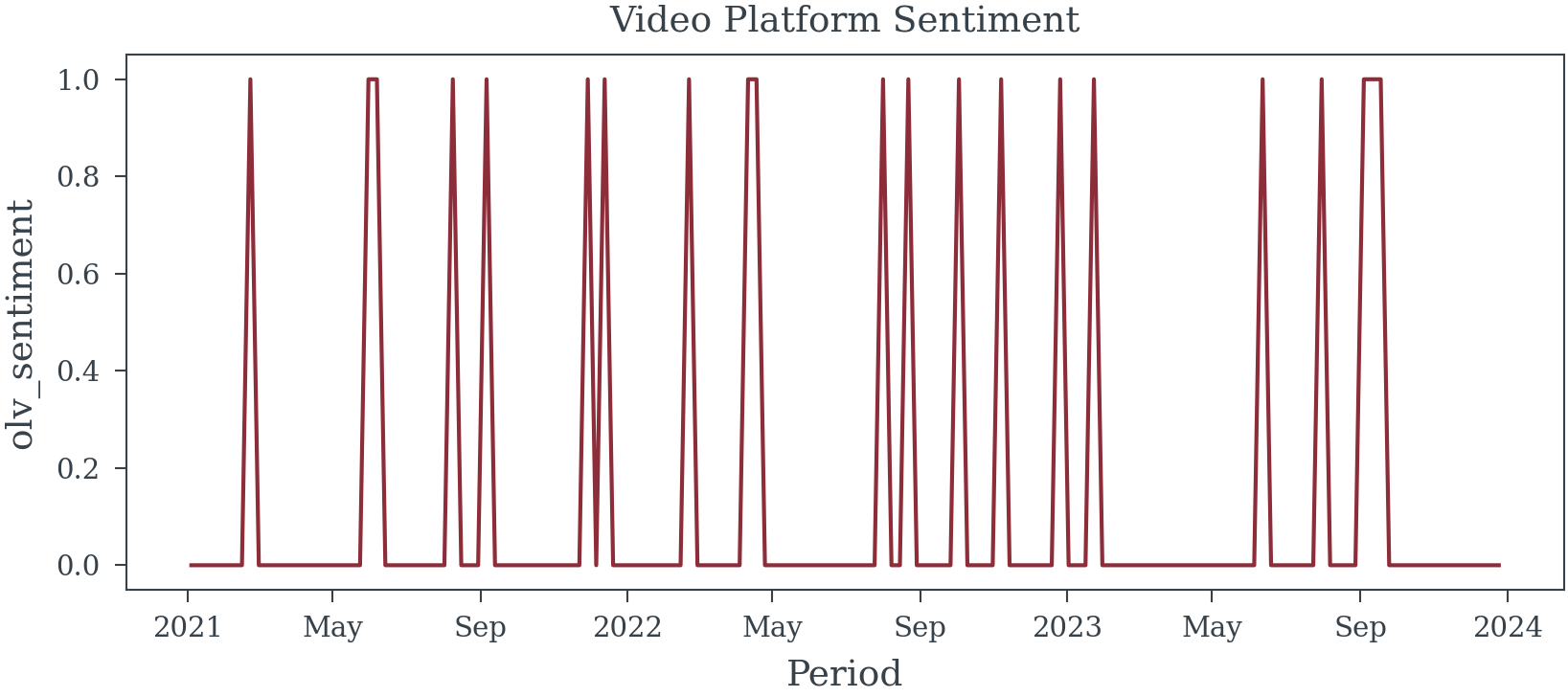
From the causal model, we can see that seasonality is part of the necessary adjustment set to accurately estimate the effect of OLV impressions on sales. Although seasonality is unobserved, we can reasonably approximate it using a periodic function (e.g., sine or cosine terms) to capture seasonal fluctuations over time. Let’s consider the following model were we adjust for seasonality (using fourier terms), price, olv impressions, and Video Platform Sentiment (olv_sentiment in the models). Note that Video Platform Sentiment is not a confounder, typically we would not adjust for it, but we include it here to illustrate the point that adjusting for variables that are not confounders can needlessly increase VIFs.

Over Adjusted Model
Correctly Adjusted Model

Figure 5: The causal graph for the relationship between OLV Impressions and Sales. Adjusting for Seasonality and Price closes all biasing paths, allowing for an unbiased estimate of the effect of OLV Impressions on Sales. Including Video Platform Sentement does nothing to reduce bias and only adds variance of our estimate.

Figure 6: Adjusting for Seasonality and Price closes all biasing paths, allowing for an unbiased estimate of the effect of OLV Impressions on Sales.

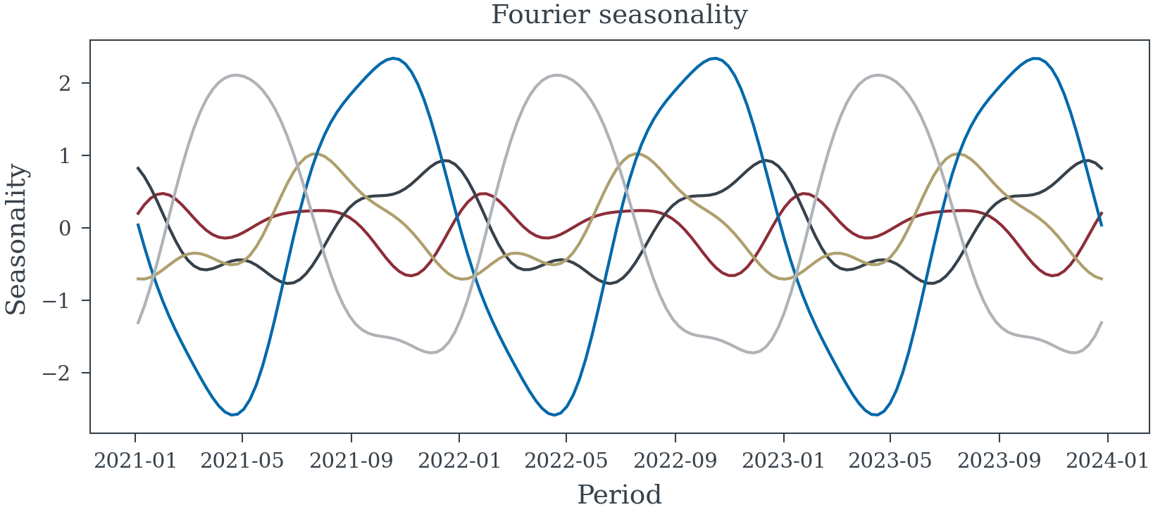
Fourier Seasonality

To capture the seasonal fluctuations in the data, we can use Fourier terms to approximate the unobserved seasonality variable. These terms are periodic functions that can model the cyclical patterns in the data, allowing us to adjust for the influence of seasonality on sales and OLV impressions. By including these terms in the regression model, we can effectively control for the confounding effect of seasonality and obtain an unbiased estimate of the effect of OLV impressions on sales.

I will use a model helper to generated the fourier

Over Adjusted Model
Correctly Adjusted Model

Table 4: VIF for the regression model with Fourier components with the addition of OLV sentiment

               VIF
hill_olv     : 70.91
log_price    : 57.59
olv_sentiment: 4.43
fourier_sin_0: 1.01
fourier_sin_1: 1.01
fourier_sin_2: 1.0
fourier_cos_0: 1.42
fourier_cos_1: 1.01
fourier_cos_2: 1.01

Table 5: VIF for the regression model with Fourier components without the addition of OLV sentiment

               VIF
hill_olv     : 18.98
log_price    : 18.84
fourier_sin_0: 1.01
fourier_sin_1: 1.0
fourier_sin_2: 1.0
fourier_cos_0: 1.14
fourier_cos_1: 1.0
fourier_cos_2: 1.0

Vectors Spaces and Basis Vectors

Fourier components provide an orthogonal basis for the space of periodic functions with a given period \(L\) . This orthogonality helps to address multicollinearity, which is why the VIFs in Table 5 and Table 4 are all near 1 for the fourier components!

Over Adjusted Model
Correctly Adjusted Model

Table 6: The over adjusted regression model with Fourier components with the addition of OLV sentiment

OLS Regression Results
Dep. Variable:	sales	R-squared:	0.888
Model:	OLS	Adj. R-squared:	0.881
Method:	Least Squares	F-statistic:	128.3
Date:	Tue, 19 Nov 2024	Prob (F-statistic):	9.51e-65
Time:	19:17:22	Log-Likelihood:	3.4816
No. Observations:	156	AIC:	13.04
Df Residuals:	146	BIC:	43.54
Df Model:	9
Covariance Type:	nonrobust

	coef	std err	t	P>\|t\|	[0.025	0.975]
const	10.7020	0.324	32.982	0.000	10.061	11.343
hill_olv	0.7217	0.433	1.665	0.098	-0.135	1.578
log_price	-1.0720	0.127	-8.433	0.000	-1.323	-0.821
olv_sentiment	0.0183	0.161	0.114	0.909	-0.299	0.336
fourier_sin_0	0.0449	0.028	1.591	0.114	-0.011	0.101
fourier_sin_1	0.0214	0.028	0.768	0.444	-0.034	0.077
fourier_sin_2	0.0166	0.028	0.596	0.552	-0.038	0.072
fourier_cos_0	-0.8321	0.041	-20.141	0.000	-0.914	-0.750
fourier_cos_1	0.1959	0.028	6.963	0.000	0.140	0.251
fourier_cos_2	0.0084	0.028	0.303	0.763	-0.046	0.063

Omnibus:	0.997	Durbin-Watson:	1.689
Prob(Omnibus):	0.607	Jarque-Bera (JB):	0.912
Skew:	-0.186	Prob(JB):	0.634
Kurtosis:	2.964	Cond. No.	53.9

Notes:
[1] Standard Errors assume that the covariance matrix of the errors is correctly specified.

Table 7: The correctly adjusted regression model with Fourier components and no OLV sentiment

OLS Regression Results
Dep. Variable:	sales	R-squared:	0.888
Model:	OLS	Adj. R-squared:	0.882
Method:	Least Squares	F-statistic:	145.4
Date:	Tue, 19 Nov 2024	Prob (F-statistic):	7.68e-66
Time:	19:18:03	Log-Likelihood:	3.4747
No. Observations:	156	AIC:	11.05
Df Residuals:	147	BIC:	38.50
Df Model:	8
Covariance Type:	nonrobust

	coef	std err	t	P>\|t\|	[0.025	0.975]
const	10.6756	0.226	47.201	0.000	10.229	11.123
hill_olv	0.7678	0.157	4.898	0.000	0.458	1.078
log_price	-1.0712	0.126	-8.468	0.000	-1.321	-0.821
fourier_sin_0	0.0444	0.028	1.597	0.112	-0.011	0.099
fourier_sin_1	0.0215	0.028	0.773	0.441	-0.033	0.076
fourier_sin_2	0.0167	0.028	0.603	0.548	-0.038	0.071
fourier_cos_0	-0.8289	0.030	-27.407	0.000	-0.889	-0.769
fourier_cos_1	0.1953	0.028	7.081	0.000	0.141	0.250
fourier_cos_2	0.0086	0.028	0.313	0.755	-0.046	0.063

Omnibus:	1.098	Durbin-Watson:	1.688
Prob(Omnibus):	0.577	Jarque-Bera (JB):	0.987
Skew:	-0.195	Prob(JB):	0.610
Kurtosis:	2.979	Cond. No.	26.6

Notes:
[1] Standard Errors assume that the covariance matrix of the errors is correctly specified.

Table 8: The correctly adjusted regression model with Fourier components and no OLV sentiment

OLS Regression Results
Dep. Variable:	sales	R-squared:	0.063
Model:	OLS	Adj. R-squared:	0.051
Method:	Least Squares	F-statistic:	5.166
Date:	Tue, 19 Nov 2024	Prob (F-statistic):	0.00674
Time:	19:27:23	Log-Likelihood:	-162.03
No. Observations:	156	AIC:	330.1
Df Residuals:	153	BIC:	339.2
Df Model:	2
Covariance Type:	nonrobust

	coef	std err	t	P>\|t\|	[0.025	0.975]
const	10.1355	0.637	15.919	0.000	8.878	11.393
log_price	-0.8167	0.355	-2.299	0.023	-1.519	-0.115
hill_olv_predicted	0.9943	0.463	2.148	0.033	0.080	1.909

Omnibus:	23.961	Durbin-Watson:	0.227
Prob(Omnibus):	0.000	Jarque-Bera (JB):	11.734
Skew:	0.487	Prob(JB):	0.00283
Kurtosis:	2.075	Cond. No.	26.5

Notes:
[1] Standard Errors assume that the covariance matrix of the errors is correctly specified.

Here, we observe that although the VIF values are considerably lower than those reported in Table 1 in the previous example (1.1.1), the impact on our ability to accurately measure the effect of OLV impressions on sales is significantly more detrimental.

Comparing Table 7 to Table 6 we see that the inclusion of Video Platform Sentiment (represented as olv_sentement in the model), did not bias the estimate of the total effect of OLV impressions on sales. However, it did lead to an increase in p-values, pushing them above our significance threshold of 0.05.

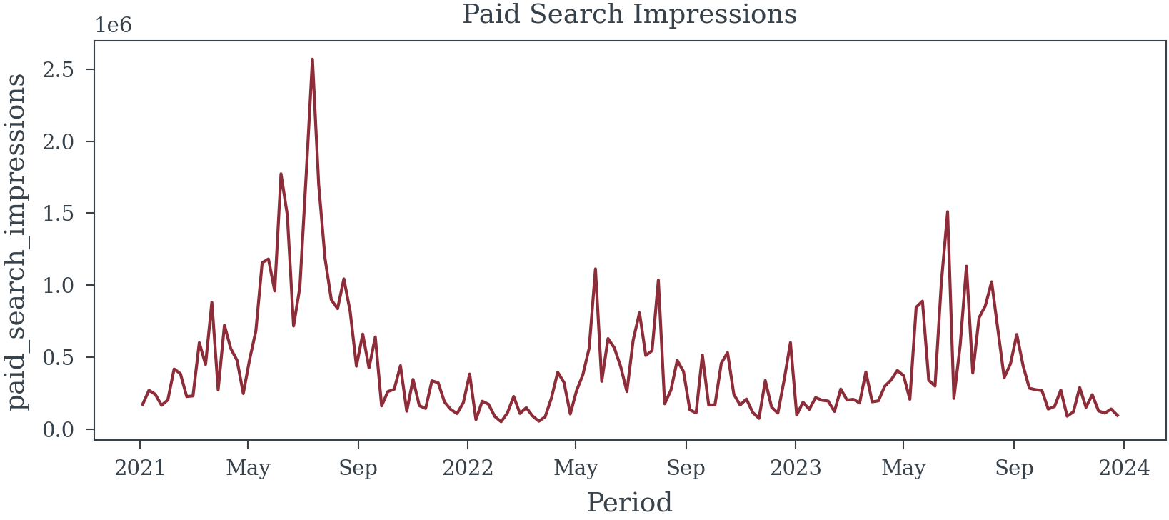
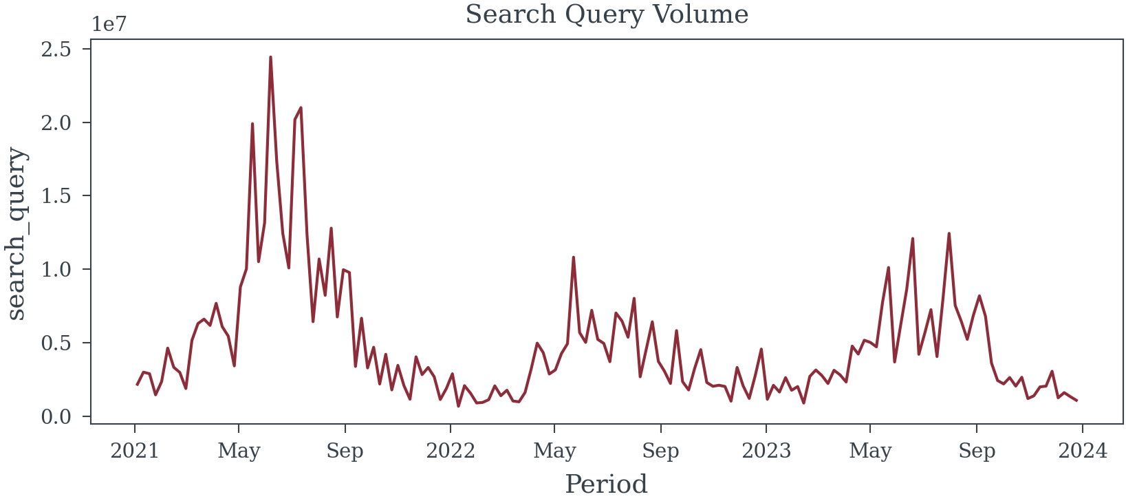
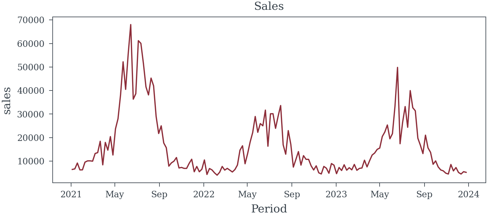
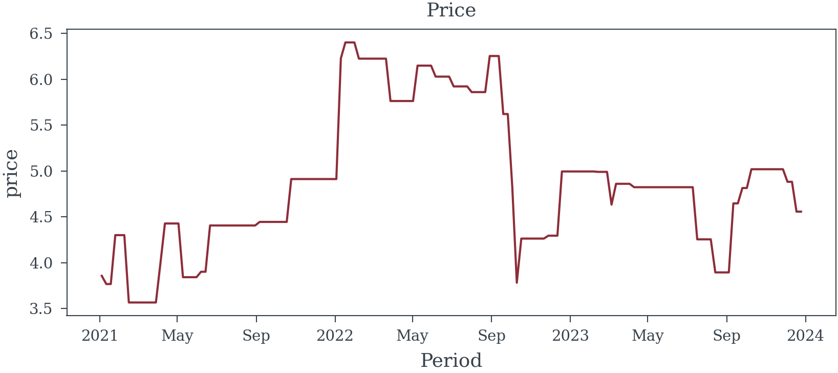
Appendix A - Paid Search Data

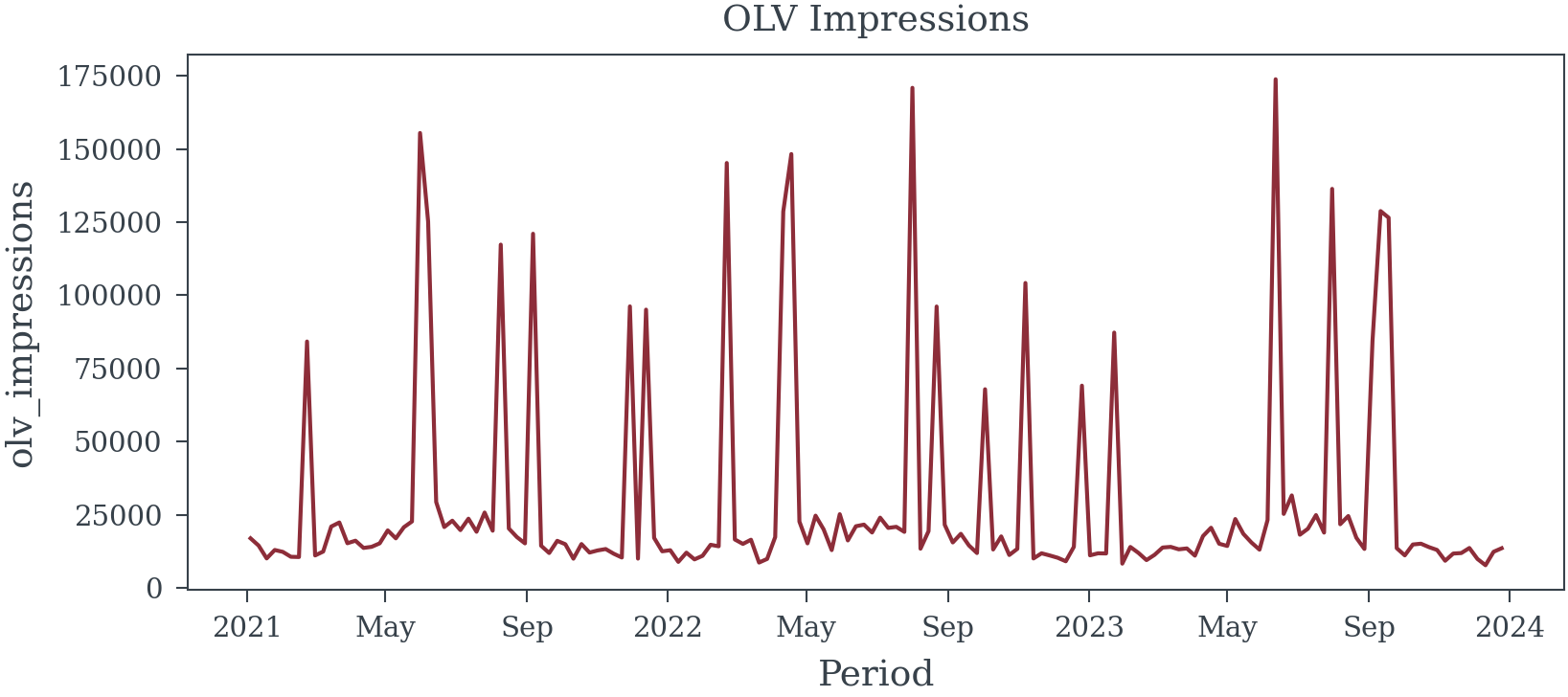
Appendix B - OLV Data

Reuse

CC BY 4.0

Citation

BibTeX citation:

@online{reda,
  author = {Reda, Matthew},
  title = {When Is {Multicollinearity} an {Issue?}},
  url = {https://redam94.github.io/common_regression_issues/multicollinearity.html},
  langid = {en}
}

For attribution, please cite this work as:

Reda, Matthew. n.d. “When Is Multicollinearity an Issue?” https://redam94.github.io/common_regression_issues/multicollinearity.html.