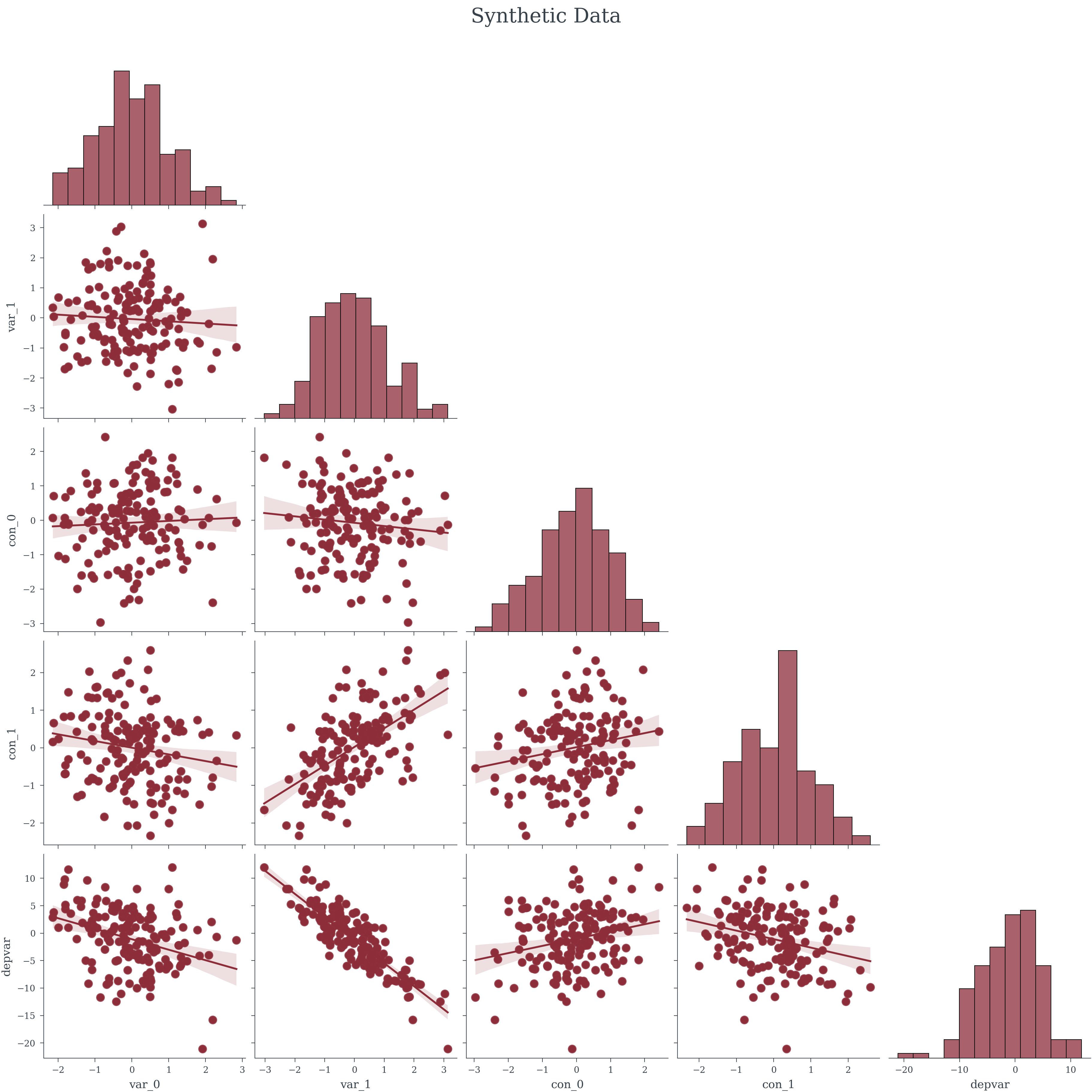
Simple Regression Data

Data simulated to adhere to standard OLS assumptions

source

generate_ols_data

 generate_ols_data (sample_size:int, n_exogenous_vars:int,
                    n_confounder:int=0, noise_sigma:float=1.0,
                    random_seed:Optional[int]=None)

Generate Simple OLS data

Type Default Details
sample_size int
n_exogenous_vars int Number of variables with a direct effect on the dep var
n_confounder int 0 Number of confounder variables to include
noise_sigma float 1.0 Level of un-explained gaussian noise to add
random_seed Optional None Random seed for reproducability
Returns Dataset Generated Data
SAMPLE_SIZE = 156
N_INDEPVAR = 2
N_CONFOUNDER = 2
NOISE_SIGMA = 1
RANDOM_SEED = 42

data = generate_ols_data(
    SAMPLE_SIZE, N_INDEPVAR, 
    n_confounder=N_CONFOUNDER,
    noise_sigma=NOISE_SIGMA, 
    random_seed=RANDOM_SEED)
data.head()
<xarray.Dataset> Size: 240B
Dimensions:  (Index: 5)
Coordinates:
  * Index    (Index) int64 40B 0 1 2 3 4
Data variables:
    var_0    (Index) float64 40B 0.5611 0.9553 -1.824 0.5083 0.162
    var_1    (Index) float64 40B -1.173 0.6022 -1.697 -1.17 -1.124
    con_0    (Index) float64 40B 1.744 0.828 0.06655 0.9896 0.7824
    con_1    (Index) float64 40B 0.439 -0.2966 -0.6974 -1.178 -0.1907
    depvar   (Index) float64 40B 2.91 -6.19 9.812 2.616 3.067
Attributes:
    true_betas:  {'var_0': -2.081, 'var_1': -4.826, 'con_0': 0.644, 'con_1': ...
    true_alpha:  -1.216
Figure 1: Sythetic Data
Table 1: OLS on synthetic data without controlling for confounds
OLS Regression Results
Dep. Variable: depvar R-squared: 0.912
Model: OLS Adj. R-squared: 0.911
Method: Least Squares F-statistic: 795.4
Date: Sat, 09 Nov 2024 Prob (F-statistic): 1.43e-81
Time: 18:17:04 Log-Likelihood: -296.16
No. Observations: 156 AIC: 598.3
Df Residuals: 153 BIC: 607.5
Df Model: 2
Covariance Type: nonrobust
coef std err t P>|t| [0.025 0.975]
const -1.2774 0.131 -9.775 0.000 -1.536 -1.019
var_0 -2.2304 0.134 -16.666 0.000 -2.495 -1.966
var_1 -4.3309 0.116 -37.226 0.000 -4.561 -4.101
Omnibus: 1.649 Durbin-Watson: 2.158
Prob(Omnibus): 0.438 Jarque-Bera (JB): 1.242
Skew: -0.188 Prob(JB): 0.537
Kurtosis: 3.223 Cond. No. 1.17


Notes:
[1] Standard Errors assume that the covariance matrix of the errors is correctly specified.
Figure 2: OLS fit on synthetic data without controlling for confounds
Table 2: OLS on synthetic data controlling for confounds
OLS Regression Results
Dep. Variable: depvar R-squared: 0.965
Model: OLS Adj. R-squared: 0.965
Method: Least Squares F-statistic: 1055.
Date: Sat, 09 Nov 2024 Prob (F-statistic): 3.26e-109
Time: 18:17:04 Log-Likelihood: -223.44
No. Observations: 156 AIC: 456.9
Df Residuals: 151 BIC: 472.1
Df Model: 4
Covariance Type: nonrobust
coef std err t P>|t| [0.025 0.975]
const -1.2551 0.083 -15.145 0.000 -1.419 -1.091
var_0 -2.1015 0.086 -24.360 0.000 -2.272 -1.931
var_1 -4.8119 0.093 -51.774 0.000 -4.996 -4.628
con_0 0.6550 0.086 7.611 0.000 0.485 0.825
con_1 1.1080 0.110 10.041 0.000 0.890 1.326
Omnibus: 1.168 Durbin-Watson: 1.685
Prob(Omnibus): 0.558 Jarque-Bera (JB): 1.216
Skew: -0.132 Prob(JB): 0.544
Kurtosis: 2.657 Cond. No. 2.21


Notes:
[1] Standard Errors assume that the covariance matrix of the errors is correctly specified.
Figure 3: OLS fit on synthetic data controlling for confounds