Some series look like they switch between a few regimes: quiet years and busy years, a resting animal and a travelling one. The natural model gives every time step a hidden discrete state and lets that state follow a Markov chain. This is a hidden Markov model (HMM), and it has a problem for anyone who samples with NUTS. The sampler needs gradients, and a state that is either 0 or 1 has none.
The way out is to never sample the states. Sum them out of the likelihood, sample the continuous parameters, and compute the state probabilities afterwards. I built a worked example around two real datasets: the yearly count of magnitude 7+ earthquakes worldwide from 1900 to 2024, and GPS tracks of four elk. The method worked. The earthquake result was less tidy than the textbook’s: on today’s catalogue, two regimes describe the series only modestly better than no regimes at all.
The generative story
A -state Poisson HMM for yearly counts reads
is the transition matrix: row says where the chain goes from state . is the distribution of the first state, and each state has its own rate . Given the path of states, the counts are independent Poisson draws. All the dependence between years runs through the hidden chain.
The data are 1,591 events over 125 years from the USGS ComCat catalogue: a mean of 12.7 a year and a variance of 17.4, where a Poisson variable would have 12.7. The autocorrelations are small, around 0.1 to 0.2, but they stay positive for twelve lags in a row, which is what slowly switching regimes would produce. This series is tamer than the one in the HMM textbook of Zucchini, MacDonald and Langrock, which covers 1900 to 2006 with a mean of about 19 a year. The old magnitudes have since been recomputed, and many events moved below 7.
Summing over paths without listing them
The likelihood of is a sum over every possible state path. With states and time steps there are paths, which is for this series with two states.
The forward algorithm gets the same sum in operations. Define the forward variable , the probability of the data so far jointly with being in state now. It obeys
It works because every path that reaches state at time passed through some state at time , and everything before that is already summed inside . The chain remembers one step, so a vector of numbers carries everything the past has to say. The Kalman filter uses the same idea for continuous states.
The recursion in PyMC
Each is a product of probabilities and underflows after a few dozen steps, so the recursion runs on the log scale, where the sum over becomes a logsumexp. The loop over time is a pytensor.scan. This is the constant-transition branch of the function in the worked example:
def hmm_loglik(log_emis, log_Gamma, log_delta):
    """log p(y_1..T) with the hidden states summed out."""
    def step(log_e_t, log_alpha, log_G_t):
        # log alpha_t(k) = log p(y_t | k)
        #   + logsumexp_j [log alpha_{t-1}(j) + log Gamma_jk]
        return log_e_t + pt.logsumexp(log_alpha[..., :, None] + log_G_t, axis=-2)

    log_alpha_1 = log_delta + log_emis[0]
    log_alpha = pytensor.scan(
        step,
        sequences=[log_emis[1:]],
        outputs_info=[log_alpha_1],
        non_sequences=[log_Gamma],
        return_updates=False,
    )
    return pt.logsumexp(log_alpha[-1], axis=-1)
sequences are sliced one emission row per step, outputs_info is the carried , and non_sequences pass through unchanged. The model computes the emission log-probabilities for every year and state, then adds the result as a pm.Potential:
coords = {"state": np.arange(K), "to": np.arange(K)}
with pm.Model(coords=coords) as model:
    lam = pm.Gamma("lam", alpha=3, beta=0.2, dims="state",
                   transform=pm.distributions.transforms.ordered)
    Gamma = pm.Dirichlet("Gamma", a=np.ones((K, K)) + 4.0 * np.eye(K),
                         dims=("state", "to"))
    delta = pm.Dirichlet("delta", a=np.ones(K), dims="state")
    log_emis = pm.logp(pm.Poisson.dist(lam), counts[:, None])  # (T, K)
    pm.Potential("hmm_loglik", hmm_loglik(log_emis, pt.log(Gamma), pt.log(delta)))
NUTS now sees a smooth function of the rates and the transition probabilities, and nothing discrete.
A hand-written likelihood needs a check. pymc_extras can write the same model generatively and remove the states itself:
with pm.Model(coords=coords_with_year) as generative_hmm:
    ...  # the same priors for lam, Gamma and delta
    regime = DiscreteMarkovChain("regime", P=Gamma,
                                 init_dist=pm.Categorical.dist(p=delta), dims="year")
    pm.Poisson("quakes", lam[regime], observed=y, dims="year")

marginal_hmm = marginalize(generative_hmm, ["regime"])
Evaluated at the same point, both log-densities came out at -364.95362, equal to six decimals. The library version is shorter. The hand-written scan is the one that can be bent later.
A failure first: label switching
Nothing in the likelihood says which state is “state 0”. Swap the two rates, the rows and columns of and the entries of , and the likelihood is identical, so the posterior has identical modes. With unconstrained rates the two-state fit reported zero divergences, an of 1.35 and a smallest bulk effective sample size of 9.
No chain had the physics wrong. Each found the same two rates, about 11 and 15, and they disagreed about the labels. In two chains each label’s mean sits near 13, between the two rates, which is what a chain that swaps labels mid-run produces. correctly reports that the chains did not sample the same distribution.
The fix is the ordered transform in the model above, which requires and keeps one mode. Ordered variables need starting values that respect the order, passed through pm.sample(initvals=...). With that, is 1.00 and the smallest bulk ESS is 969. The fit describes a quiet regime of 10.85 earthquakes a year (94% HDI 9.11 to 12.33) and a busy one of 14.77 (13.08 to 16.31), each persisting from one year to the next with probability about 0.89.
Getting the states back
The states were summed out, not lost. A mirror-image recursion run backwards gives , and for each posterior draw
Averaging over draws gives the smoothed probability of each state in each year. The worked example runs this in NumPy on all 4,000 draws at once, after sampling. The pymc_extras route is recover, which samples one state path per draw. The two answers differed by at most 0.011.
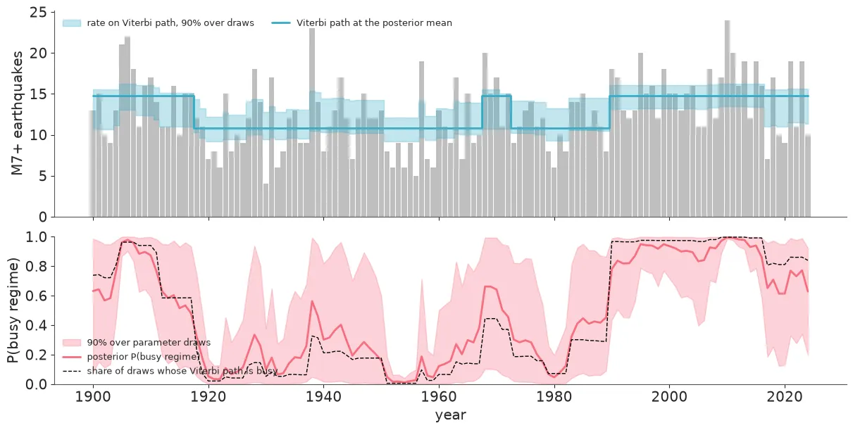
The worked example’s own figure. The band in the lower panel is the spread of the busy-regime probability across parameter draws.
There is a busy stretch around 1905 to 1915, brief bumps in the late 1930s and around 1970, and a long busy period from about 1990 to the mid-2010s. The band matters more than the line. For most years the probability of the busy regime ranges over half the unit interval across parameter draws. The two rates are about four earthquakes a year apart and a Poisson count here has a standard deviation of about 3.5, so one year cannot tell them apart. The assignment comes from runs of years. The Viterbi algorithm finds the single most probable path and commits every year to one state, so the share of draws whose path is busy sits closer to 0 or 1 than the smoothed probability does.
Persistence is just as uncertain. The median dwell time is 12 years in the quiet regime and 11 in the busy one, with 94% intervals of 2 to 60 and 2 to 43 years. The prior on each row of mildly favours staying (a Beta(5, 1) for two states, mean 0.83). Replacing it with a flat prior moved the stay probabilities from 0.89 to about 0.76 while the rates barely changed. A handful of switches in 125 years cannot pin down how sticky the regimes are.
How many states, and are they regimes at all
The hidden state does carry information. One-step-ahead forecast residuals from a plain Poisson model keep the series’ autocorrelation (0.16, 0.16 and 0.20 at lags 1 to 3), and the HMM’s do not (-0.02, 0.02 and 0.10). Series replicated from the plain Poisson posterior matched or exceeded the observed variance-to-mean ratio 0.7% of the time. The HMM’s did 26.6% of the time.
More states did not help. Three states produced 5 divergences and four produced 32, and the rates of neighbouring states overlap.
The extra states are slices of the same two, and a rarely visited state has its rate pinned only by the prior. This is a modelling result. Raising target_accept would hide the divergences without making the extra states real, and the ordering constraint does not help either: when two rates overlap, it cuts a multimodal posterior in an arbitrary place.
Comparing models takes care because the years are not independent given the parameters. The worked example uses leave-one-out with the states integrated out, which reuses the forward and backward variables with no refit, and a forecasting test: fit on 1900 to 1989, then score the 35 years from 1990 to 2024 one step ahead.
| Model | Integrated LOO: elpd behind the best (SE) | Forecast: elpd ahead of one rate (SE) |
|---|---|---|
| Three-state HMM | 0.0 (best) | not run |
| Two-state HMM | 0.0 (0.6) | 5.4 (2.3) |
| Four-state HMM | 0.1 (0.5) | not run |
| Negative binomial, i.i.d. | 3.1 (3.4) | 2.0 (1.5) |
| One Poisson rate | 5.9 (4.4) | 0.0 |
The two-state HMM beats a single rate by a few units with standard errors of a few units, and it is not decisively better than “more variable than Poisson, with no time structure”. That is weak evidence for regimes. It is also not a physical claim: a catalogue that mixes magnitude types over a century can mimic regimes.
The same scan, bent
The reason to keep the hand-written recursion is the second dataset: 735 GPS locations of four elk, with a step length and a turning angle for each move. Each change is one line. The four tracks become a batch axis, padded to the longest. A missing or padded observation gets a log-emission of 0, which means “no information at this step”. Two emissions add their log-densities.
The fit separates an encamped state, with a mean step of about 0.38 km and turning angles centred on reversals, from an exploring state with a mean step of about 3.4 km. Letting the transition probabilities depend on distance to water uses the same scan with one matrix per step. An exploring elk is more likely to settle the farther it is from water (slope 1.22 per standard deviation of distance, 94% HDI 0.33 to 2.13). The integrated LOO still put that model only 2.0 units of elpd ahead with a standard error of 3.9: no demonstrable gain in predicting individual steps. And for one elk the step residuals stayed positively autocorrelated at every lag, so two states did not capture everything.
What to do in practice
- Sum the states out. Write the forward recursion on the log scale and check it at one point against
marginalizefrompymc_extras. - Break the label symmetry on purpose. Order the parameter that separates the states and pass ordered starting values. The constraint only works when the states differ clearly in that parameter.
- Report state probabilities with their spread. The state sequence is a summary of a posterior, not an observation.
- Read divergences after adding states as an answer. Overlapping rates and divergences mean the data do not support the extra state.
- Compare against a dull overdispersed model, with the states integrated out, and with a forecast test if forecasting is the point.
- Report persistence with its prior. With few observed switches, the prior on visibly moves the answer.
The states of an HMM are a modelling device. “Busy regime” is a label for a mixture component with Markov dynamics, and it will absorb a trend or a catalogue change as if it were a state. Marginalising makes the model easy to fit. It does not make the states real.
Further reading: the full worked example has the data, the complete models, the checks and the elk analysis. All empirical numbers above come from it. It is a modelling lesson, not a seismological finding. References as cited there: Zucchini, MacDonald & Langrock (2016) for the Poisson HMM and its earthquake series; Morales, Haydon, Frair, Holsinger & Fryxell (2004), Ecology 85:2436, for the elk tracks, as shipped with the R package moveHMM.