Population Pharmacokinetics Is a Compartment Model Inside a Hierarchy

Most regression functions are chosen for convenience: a line, a spline, a tree. In pharmacokinetics the regression function is the solution of a differential equation, and its parameters are physical quantities with units: a clearance, a volume, an absorption rate. Every person has their own values, and nobody gives enough blood to pin theirs down alone. A mechanistic curve per person, with a distribution over people on top, is a population pharmacokinetic model.

I built a worked example on two classic datasets. This post covers the first: theophylline, 12 subjects, one oral dose each, 120 post-dose concentrations over 25 hours. It is a statistics post. The dosing analysis at the end is a modelling exercise on a study subject, not guidance for treating anyone.

The regression function is a compartment model

Treat the body as one well-mixed volume $V$. Drug enters from the gut at a rate proportional to what is still there, with rate constant $k_a$, and leaves at a rate proportional to the concentration, with rate constant $k_e$. Those are two linear differential equations with a closed-form solution. For a dose $D$:

$C(t) = \frac{D\,k_a}{V\,(k_a - k_e)}\left(e^{-k_e t} - e^{-k_a t}\right), \qquad k_e = \frac{CL}{V}$

$CL$ is the clearance, the volume of plasma cleared of drug per hour. It is the parameter that sets exposure, because the area under the curve is $D / CL$. The worked example adds one term, $C_\text{pre}\,e^{-k_e t}$, for the three subjects who had a little theophylline in their blood before the dose.

The formula has a removable 0/0 at $k_a = k_e$, and a sampler will wander near it. The example rewrites the difference of exponentials with expm1, which stays accurate on both sides:

def conc_pt(CL, V, ka, t, dose, c_pre=0.0):
    """One-compartment oral model (PyTensor), valid for ka > ke and ka < ke."""
    ke = CL / V
    delta = ka - ke
    return (dose * ka / V * pt.exp(-ke * t) * (-pt.expm1(-delta * t)) / delta
            + c_pre * pt.exp(-ke * t))

That function is the whole mean structure. Everything around it is a hierarchical regression.

Why the parameters get a population distribution

Each subject has ten post-dose samples and three parameters. Fitting each person separately gives noisy estimates and says nothing about a thirteenth person. Pooling everyone into one curve is wrong on sight: on a log scale the concentrations fall along nearly straight lines whose slopes differ between people. The hierarchy sits between the two. Each subject’s log-parameters are a draw from a shared multivariate normal:

$\theta_i = \mu + L z_i, \quad z_i \sim \mathcal{N}(0, I), \qquad y_{ij} \sim \mathcal{N}\!\left(C(t_{ij};\theta_i),\ \sqrt{(\sigma_\text{prop} C)^2 + \sigma_\text{add}^2}\right)$

$\mu$ is the typical subject, and $L$ is the Cholesky factor of the between-subject covariance, with an LKJ prior on the correlations. Working on the log scale keeps every parameter positive and makes the population log-normal. The non-centred form ($\mu + L z_i$) is the usual choice for a dozen groups. The residual error has a proportional part and an additive floor, the common shape for assay error.

MU_PRIOR = np.array([np.log(0.04), np.log(0.5), np.log(1.5)])
SD_PRIOR = np.array([0.5, 0.3, 1.0])

with pm.Model(coords=coords_pop) as m_pop:
    mu = pm.Normal("mu", MU_PRIOR, SD_PRIOR, dims="par")
    chol, _, _ = pm.LKJCholeskyCov("L", n=3, eta=2.0,
                                   sd_dist=pm.HalfNormal.dist(0.5), compute_corr=True)
    z = pm.Normal("z", 0.0, 1.0, dims=("subj", "par"))
    theta = mu + z @ chol.T
    CL = pm.Deterministic("CL", pt.exp(theta[:, 0]), dims="subj")
    V = pm.Deterministic("V", pt.exp(theta[:, 1]), dims="subj")
    ka = pm.Deterministic("ka", CL / V + pt.exp(theta[:, 2]), dims="subj")  # ka > ke
    c = conc_pt(CL[sid], V[sid], ka[sid], t_obs, dose_kg[sid], c_pre[sid])
    sig_prop = pm.HalfNormal("sig_prop", 0.2)
    sig_add = pm.HalfNormal("sig_add", 0.5)
    pm.Normal("y", c, pt.sqrt((sig_prop * c) ** 2 + sig_add**2), observed=y_obs)

Two lines in that model are not routine: the informative prior on the volume (centre $\log 0.5$, sd 0.3) and the definition of ka as CL / V plus a positive excess. Both exist because of what happens without them.

Where it breaks: a mirror-image posterior

Swap $k_a$ and $k_e$ in the formula. The bracket changes sign and so does the denominator, so the shape of the curve is unchanged. Only the prefactor moves, and choosing $V' = V k_e / k_a$ cancels that as well. A body that absorbs slowly and eliminates fast, with a much smaller volume and the same clearance, draws the identical curve at every time. Pharmacologists call slow absorption that looks like elimination flip-flop kinetics.

A hierarchy does not rescue this, because the whole population can flip together. The worked example fits a version with vague, unordered priors and starts two chains in each world. Each chain stayed where it started. The run reported 72 divergences, all from the mirror chains, a largest r_hat of 1.759 and a smallest bulk effective sample size of 6. All four chains agreed on the typical clearance (0.040 or 0.041 L/h/kg) and fitted the data equally well, with mean log-likelihoods within about 1. The mirror chains described a population with a typical volume of 0.028 L/kg.

The r_hat alarm was correct, but it rang only because the chains were deliberately started in both basins. A single run that happened to start in one of them would have looked healthy.

Two kinds of information break the symmetry, and they assume different things. The ordering $k_a = k_e + e^{\eta}$ keeps only the branch where absorption is faster. That is true for an immediate-release oral solution like this one and false for sustained-release products, where the ordering would silently pick the wrong world. The physiological prior on $V$ does not care which rate is faster: theophylline distributes in body water, about 0.5 L/kg, and the mirror mode sits about 9 prior standard deviations away. The example uses both.

What the fit showed

With both in place the model sampled with 0 divergences, a largest r_hat of 1.005 and a smallest bulk effective sample size of 684. The typical subject clears 0.040 L/h per kg (90% interval 0.035 to 0.047) from a volume of 0.46 L/kg, a half-life of about 8 hours. Clearance varies between people with a coefficient of variation of about 27%, and absorption varies far more (log-scale sd 0.75). The data did the work on clearance: the prior’s 90% interval for the typical value was 0.018 to 0.091. They did less for the correlation between clearance and volume, whose median is 0.6 with a 90% interval from 0.04 to 0.90.

The checks were less tidy. LOO could not separate the combined error model from a purely additive one (a difference of 0.4 with a standard error of 3.1, and 6 or 7 observations with Pareto $\hat k$ above 0.7 in each, so the comparison is itself approximate). The individual fits miss sharp early peaks: subjects 1, 5 and 9 each have a sample in the first hour or so at or above the upper edge of their band. Normalised prediction errors show no drift, but their spread is wide in the first two hours and narrow afterwards, with an overall sd of 0.77. The model is adequate for clearance and the elimination phase and weakest in absorption.

The second half of the example, on warfarin, has a failure of the same family. A lag-time parameter created a spurious mode: one of four chains sat at a lag near 1 hour with a mean log density about 19 units lower, r_hat reached 1.13, and there were no divergences. Starting the lag at 0.6 hours without jitter fixed it.

Partial pooling for a subject with two samples

Before any blood test, a new person is a draw from the population. Add them to the model as one more subject with two observations, and their posterior combines the population, acting as the prior, with their own samples. Nothing new has to be built.

The example tests this on real people. For each subject in turn it refits to the other 11 plus two of that subject’s samples, those nearest 7 and 24 hours, and predicts the eight that were held out. The same fit carries a “ghost” subject with no data, whose parameters are the population-only forecast. One compiled model serves all twelve fits, because the likelihood weights are data:

w = pm.Data("w", np.ones(len(y_obs)))
pm.Potential("loglik", (w * pm.logp(pm.Normal.dist(c, sig), y_obs)).sum())

compiled_tdm = nutpie.compile_pymc_model(m_tdm)
tr = nutpie.sample(compiled_tdm.with_data(w=w), seed=RANDOM_SEED + k)

Over the 96 held-out concentrations the gain depends on the phase. After 4 hours the mean absolute error halves, from 0.85 to 0.42 mg/L. Over all held-out samples it falls only from 1.34 to 1.11, because the early samples depend on the absorption rate, which samples at 7 and 24 hours say almost nothing about. The 90% predictive intervals covered 93% to 95% of the held-out values in both cases. The 90% width of each subject’s clearance posterior halves on average, from 0.041 to 0.021 L/h/kg.

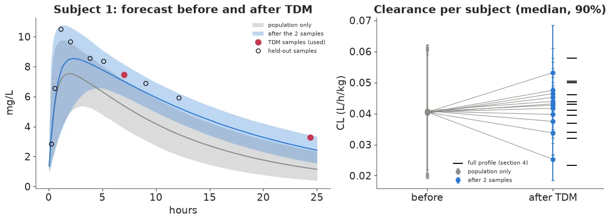
Subject 1 clears theophylline more slowly than anyone else in the study. The population forecast falls off too fast. Two samples pull the forecast through the held-out points after 2 hours, though the sharp early peak is still under-predicted.

From a posterior to a regimen

Under repeated dosing the steady-state curve is a superposition of the single-dose solution. It is again closed-form and linear in the dose, so each posterior draw yields a peak and a trough per milligram, and any candidate regimen gets a probability. The example’s target is the classical 10 to 20 mg/L range for theophylline (it notes that some current guidelines aim lower), held through the whole dosing interval. The probability of target attainment is the share of draws whose trough is at least 10 and whose peak is at most 20.

For subject 1 the example scans doses from 50 to 1,000 mg in 25 mg steps at intervals of 6, 8 and 12 hours. With the population alone, the best regimen is 275 mg every 6 hours, and it reaches the target with probability 0.50: the spread in clearance between people is wider than the window allows. After two samples the best dose drops to 175 mg every 6 hours with probability 0.84, the same dose the full profile picks. Judged with the two-sample posterior, the population-based 275 mg would put the peak above 20 mg/L with probability 0.91. At a 12-hour interval nothing works well: the best dose reaches the target with probability 0.35 after two samples and 0.46 with the full profile.

These probabilities are conditional on the model. The example states two caveats: the steady-state predictions assume linear kinetics while theophylline’s elimination is known to saturate at high concentrations, and the posterior comes from a single-dose study. It adds that a real monitoring service would confirm with a steady-state trough sample.

What to do in practice

1. Write the mechanistic solution as a plain function first. A closed form in a numerically stable arrangement is easier to test than a model block, and it is reused for every prediction afterwards.

2. Look for symmetries on paper, then start chains on both sides. r_hat can only compare the chains it is given.

3. Break a symmetry with knowledge you can defend, and say which. An ordering constraint assumes fast absorption. A physiological prior on the volume does not.

4. Put positive parameters on the log scale, non-centre them, and model their correlation. Then report how little a dozen subjects say about that correlation.

5. Validate the pooling out of sample. Hold out most of one subject’s data, keep a no-data subject in the same fit as the population baseline, and compare the two forecasts.

6. Report the decision as a probability under a stated state of knowledge. List the assumptions the posterior does not cover next to it.

The compartment model supplies the shape of the curve, the hierarchy supplies the prior for the next person, and two samples were enough to move one subject’s regimen. The example’s own checks also show where the same model is weak: the first two hours.

Further reading: the full worked example has the data, the complete models, the warfarin covariate and clotting-response analysis, and the figures behind every number above. All empirical numbers in this post come from it. It is a modelling lesson, not medical advice. Data: Boeckmann, Sheiner & Beal (1994), NONMEM Users Guide Part V, as distributed in R’s datasets::Theoph.