Explore a model v0.5

The Model Explorer shows what a fitted model learned and how well it works. It does this for all model families:

• Bayesian: posterior means with highest-density intervals, and R-hat.
• Frequentist: estimates with confidence intervals and p-values, and information criteria.
• Machine learning: coefficients or importances.

The sandbox calculates the views from the bundle and the data that the fit used. The views come with Vega-Lite plots. The web app shows each section with governance evidence and lineage. It also compares versions and optimises budgets. The rest of this guide uses the HTTP API that the web app calls.

In the web app

The page of a model version has Explore and Compare. For marketing-mix models, it also has Optimise budget. The Model Explorer (/models/<model>/versions/<n>/explore) puts its sections into groups by the question that they answer:

Group	Sections
Overview	At a glance: the plain readings of the diagnostics and the fit, the holdout metrics and the About card of the model
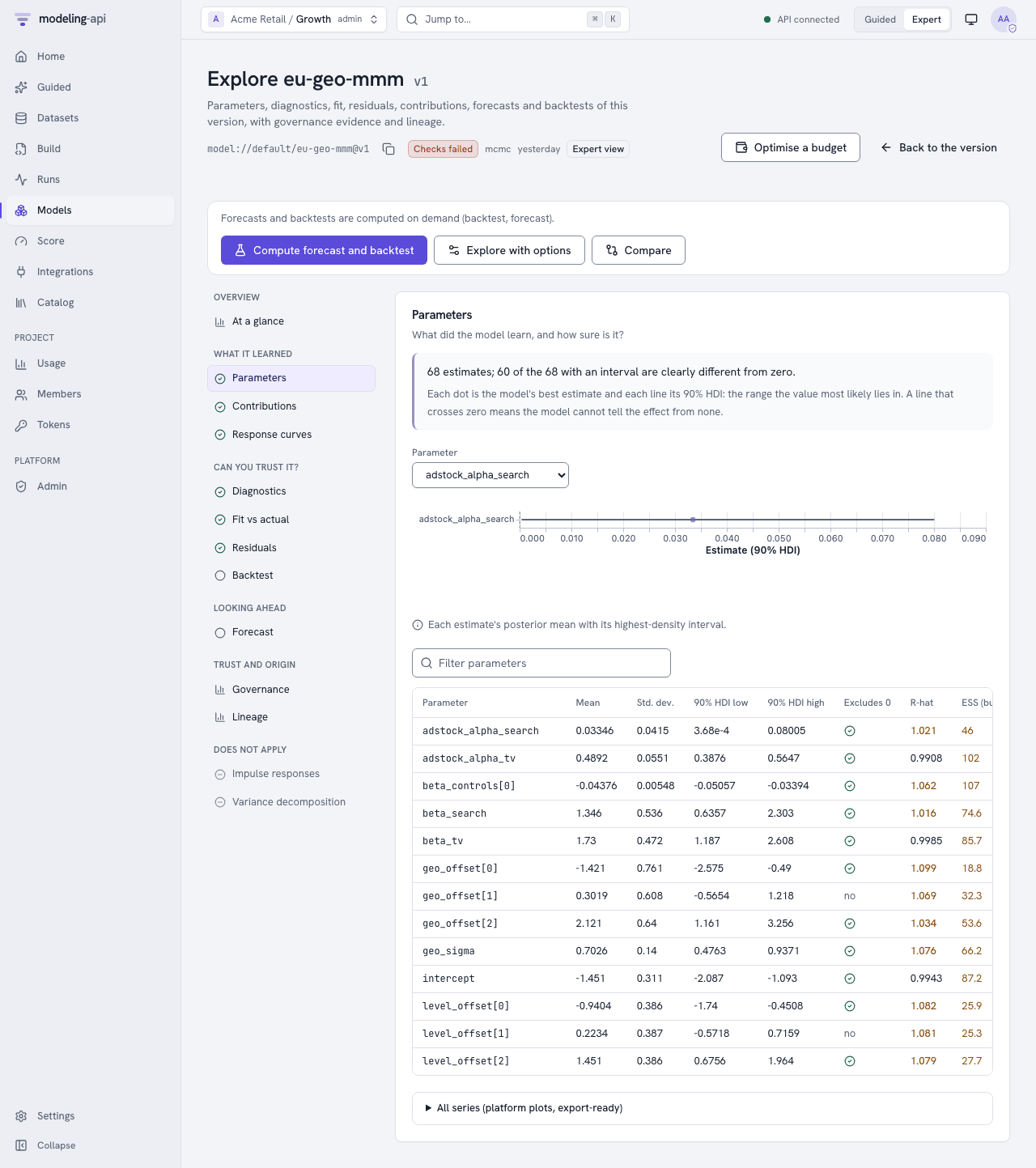
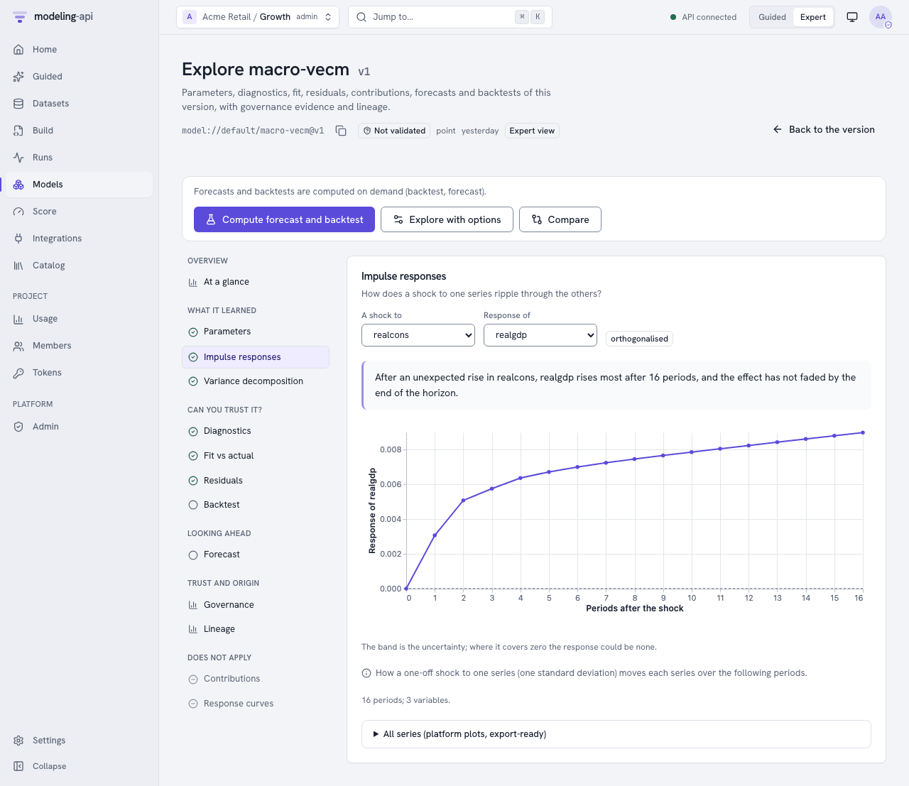
What it learned	Parameters (a table that you can sort and filter, with intervals, p-values, R-hat and ESS, and a forest plot for each parameter), contributions, response curves, impulse responses, variance decomposition and fields (the outputs of the model on a 2-D grid)
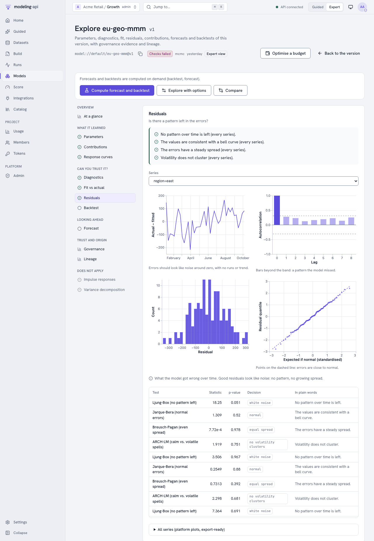
Can you trust it?	Diagnostics (convergence, fit statistics for each series, the tests of the model), fit vs actual (with the coverage of the band in plain words), residuals (over time, ACF, histogram, QQ plot, Ljung-Box, Jarque-Bera, Breusch-Pagan and ARCH-LM), backtest
Looking ahead	Forecast (a fan for each series)
Trust and origin	Governance (the status badge of the latest validation, each check with its evidence, the status history) and lineage (dataset, spec revision, fit run and workflow run, and also plugin, image, seed and libraries)

The explorer lists the sections that do not apply to the model last, with the reason. For example, an MMM has no impulse responses. The explorer calculates forecasts and backtests only when you ask:

• Click Compute forecast and backtest.
• Or click Explore with options. Then set the horizon, the interval and the backtest plan. The plan has these items: expanding window or rolling origin, horizons, folds, minimum training periods and gap.

As in the Data Explorer, Guided mode shows the plain reading first. Expert mode shows all the numbers.

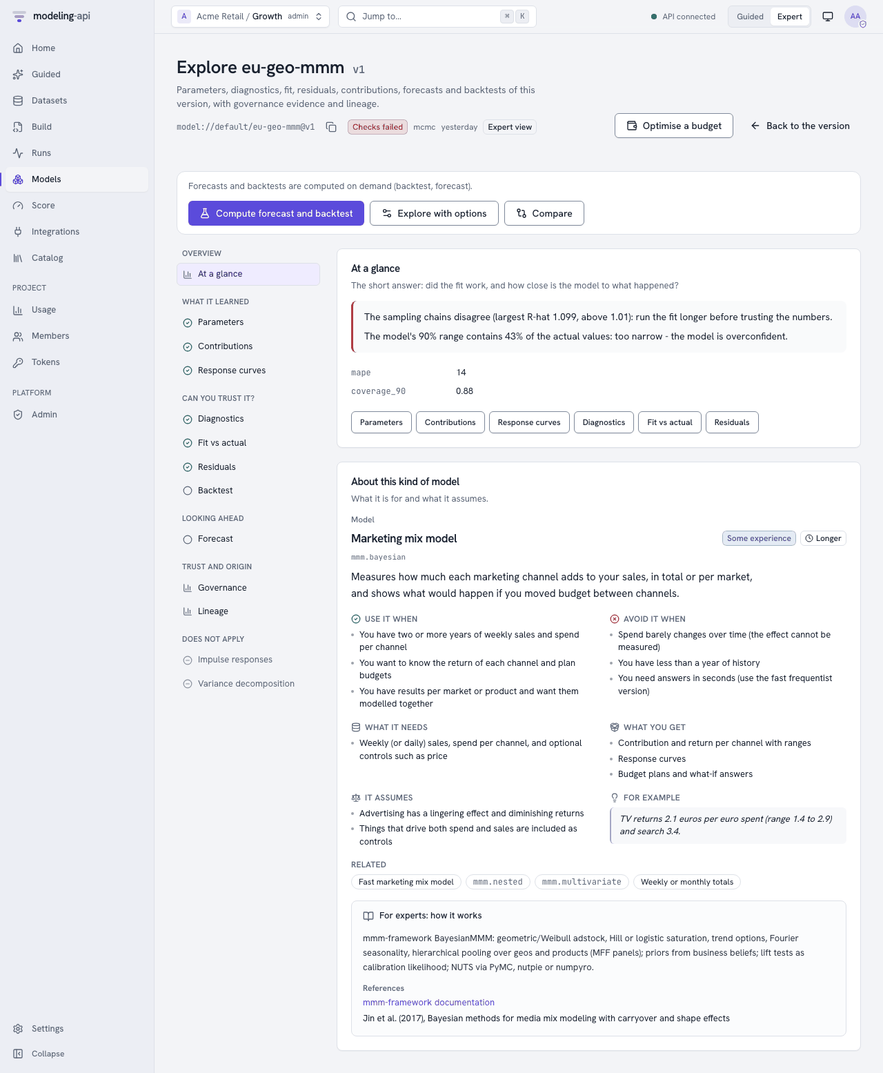
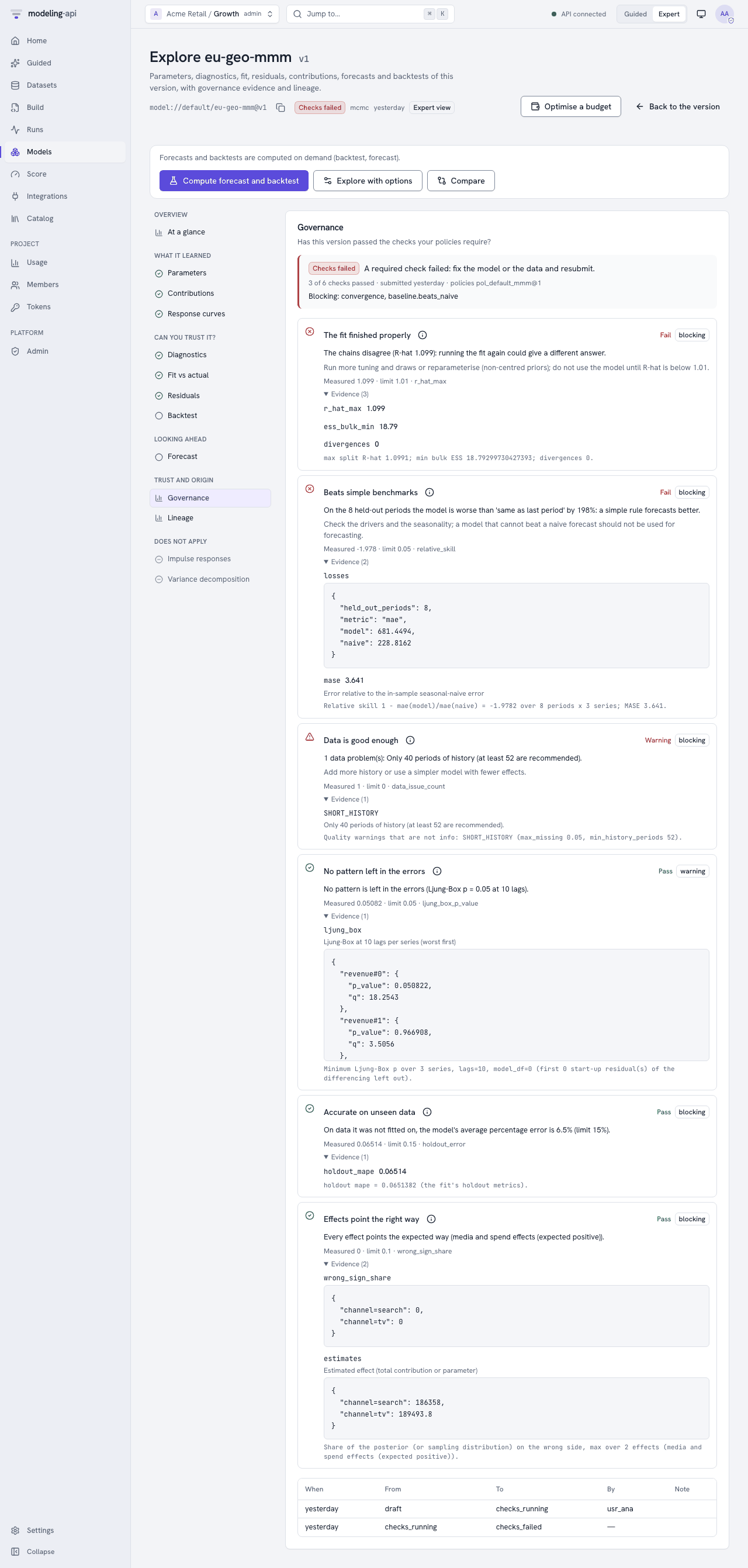
The header shows the validation status of the version. It has a link to the validations of the version, where you can request a new validation. Under Governance evidence, these links show:

• Open this validation goes to the latest validation: its status path, the decisions of the reviewers and the evidence pack.
• Policies goes to the governance policies. See Validate models with governance policies.

If a workflow fitted the version, Lineage has a link to the monitor of the workflow run.

Compare (/models/compare) shows two to eleven versions side by side. To use it:

1. Select each model and version. The tests use the first version as the reference.
2. Click Compare.

The page shows these items:

• The holdout metrics, with a mark on the best value of each metric.
• The Diebold-Mariano tests in plain words. For example, "about equally accurate", or an advantage that is more than chance.
• The ranking for each metric.
• The fit statistics of each version.
• Which version predicts new data best? (v0.10): the core.model_comparison plot. It shows the expected log predictive density (elpd) of each version and its difference to the best version. The card shows only when two or more versions have elpd_loo (or elpd_waic) on the same number of observations. The description of the card tells you which of the two estimates the plot shows.

Time-series forecasters (statsmodels and the other ts models) forecast the full held-out period from one origin. Thus their errors make a single path, and no test of equal accuracy is valid on it. For these models, the page shows the metrics and rankings. It tells you to compare their backtests. You can also run a compare.diebold_mariano workflow node on rolling-origin backtest errors.

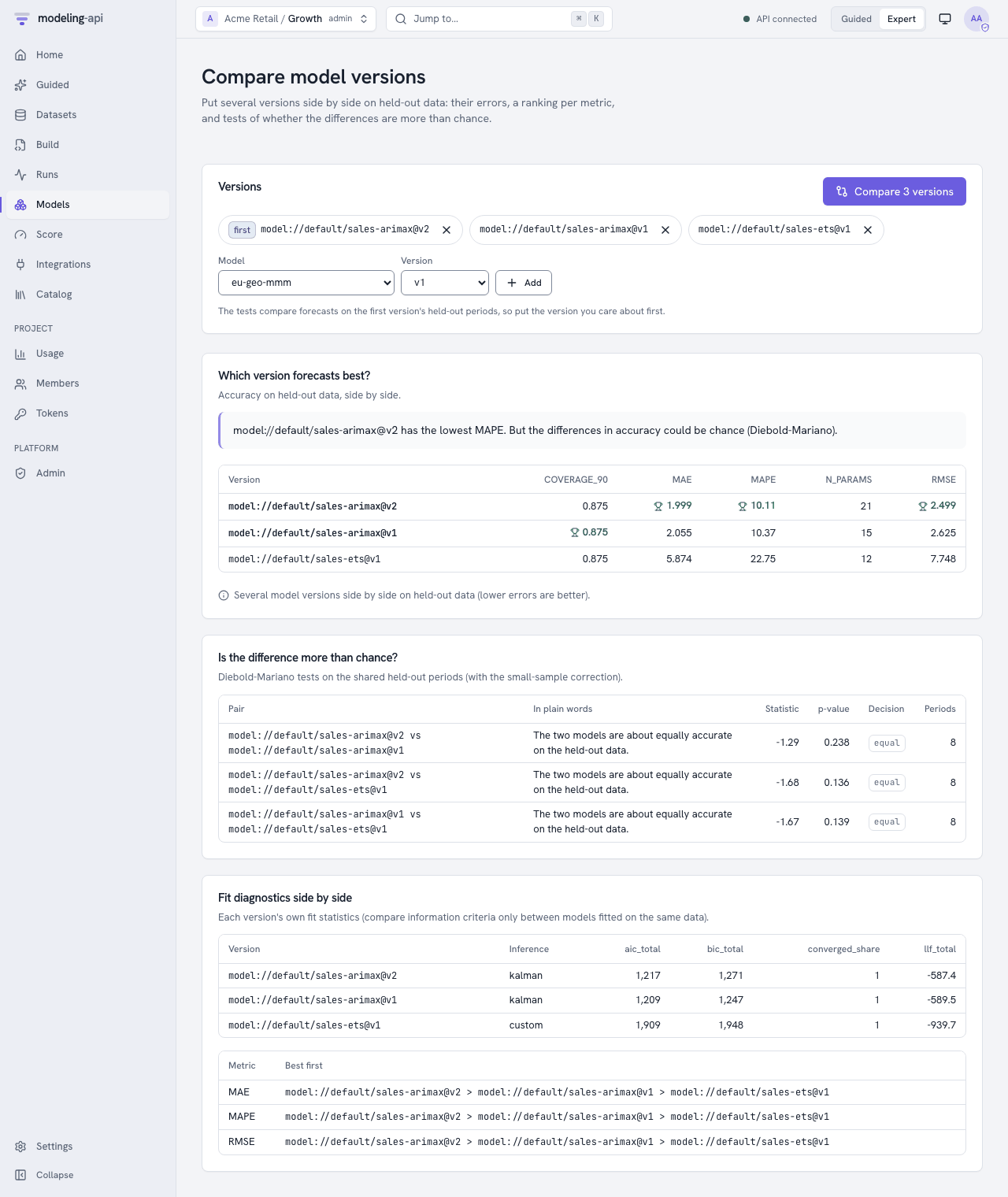
Compare compares model versions on held-out data. To compare the runs of a study (the metrics, params, curves and images that each run logged), use the compare page of the runs table. See Compare runs and use experiments.

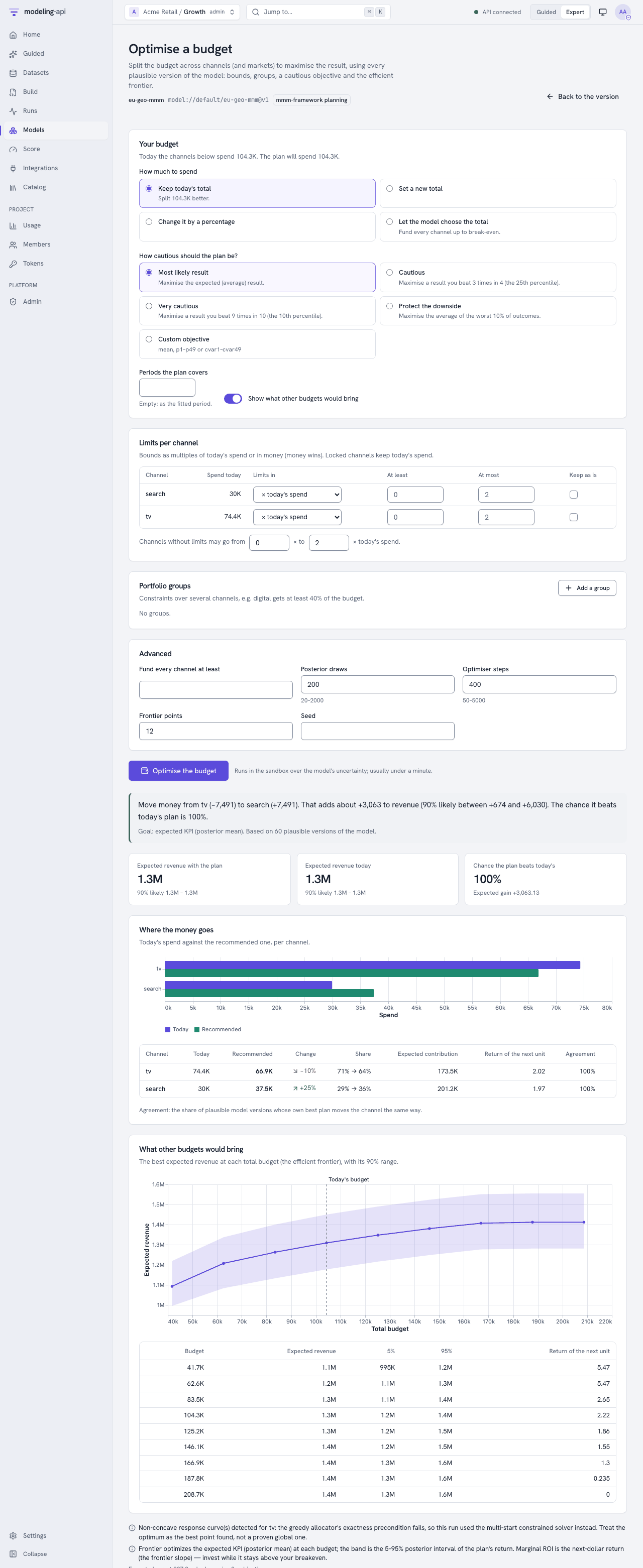
Optimise budget (/models/<model>/versions/<n>/optimize) is only for marketing-mix models. It asks for these items:

• How much to spend: the current total, a new total, a change in percent, or the total that the model would select. The last option is only in Expert mode.
• How careful to be: the expected result, the 25th or 10th percentile, or the average of the worst 10%.
• Limits for each channel: multiples of the current spend, an amount of money, or no change.
• Portfolio groups and the frontier.

If the page cannot meet a bound, it tells you why before anything runs. The plan reads like this: "Move money from tv (−7,491) to search (+7,491). That adds about +3,063 to revenue (90% likely between +674 and +6,030)…". The plan also shows these items:

• The allocation for each channel (and market).
• The expected result now and with the plan.
• The probability that the plan is better than the current allocation.
• The return of the next unit for each channel.
• The efficient frontier.

The expected results show the number of digits that is necessary to make the two ends of each range different. For example, "1.305M – 1.312M", not "1.3M – 1.3M". In Guided mode, the What if… step goes to this page with Optimise my budget. The page gives the goal and the notes of the optimiser in plain words, for example "Goal: the most likely revenue". The text of the optimiser itself is under For experts: how the plan was found. The request and the result are the request and result of POST …:optimize.

From Python and the command line

model_id, version = "mdl_01jaf3c1d2e3f4g5h6j7k8m9n0", 3
explored = api.models.explore(
    model_id, version, sections=["params", "residuals", "forecast"], horizon=13
)
residuals = api.explorations.view(explored, "residuals")

compared = api.models.compare(
    ["model://growth/arimax@v3", "model://growth/ets@v1", "model://growth/theta@v2"], horizon=4
)
table = api.explorations.view(compared, "comparison")  # metrics, ranking, Diebold-Mariano

mapi explore model model://growth/sales-arimax@v2 -s params -s residuals -s irf --horizon 12
mapi explore compare model://growth/sales-arimax@v2 model://growth/sales-ets@v1 --horizon 4

Views written at fit

Each fit writes params, diagnostics, fit, residuals, decomposition, response_curves, irf, fevd and fields. The fit lists the sections that do not apply to the model as skipped, with the reason. Read the index and the views through the UI route of the model version:

api "$API/v1/models/$MODEL_ID/versions/3/artifacts/ui/explore/index.json"
api "$API/v1/models/$MODEL_ID/versions/3/artifacts/ui/explore/residuals.json"

Forecasts, backtests and more, on demand

api -X POST "$API/v1/models/$MODEL_ID/versions/3/explore" -d '{
  "sections": ["forecast", "backtest"],
  "horizon": 12,
  "backtest": {"kind": "expanding_window", "horizons": [1, 4, 12], "n_folds": 5,
               "min_train": 104}
}'

The answer (202) is an Exploration. Poll GET /v1/explorations/{run_id} to get the index and the signed view links. If you send the same request again, the answer is 200 from the last run.

Error by horizon v0.11

The backtest view has the error metrics for each horizon, pooled over all the folds (BacktestView.by_horizon, for example by_horizon["4"]["mae"]). Each fold also keeps its own by_horizon. If the plan has no horizons, the backtest uses the horizons 1 to the length of the first test window (a maximum of 32).

The backtest section has a second chart, "Backtest error by horizon". It shows the pooled MAE for each number of periods ahead, and a light line for each fold. The chart shows only when two or more horizons have a pooled MAE. The error usually increases with the horizon. A fast increase tells you that the model is good only for short forecasts.

Compare model versions

api -X POST "$API/v1/models:compare" -d '{
  "models": ["model://growth/sales-arimax@v3", "model://growth/sales-ets@v1",
             "model://growth/sales-mmm@v2"]
}'

This call explores the first version with the other versions as compare_with. It writes the comparison view, which has these items:

• The holdout metrics of each version, side by side.
• A ranking for each error metric. A lower value is better.
• Pairwise Diebold-Mariano tests on the held-out periods of the first version. The tests use the Harvey-Leybourne-Newbold small-sample correction and a Newey-West number of autocovariances. They answer the question "is the difference in accuracy more than chance?".
• The core.model_comparison plot (v0.10), in ui/explore/plots/comparison.json after the metric bars. The view adds it when two or more versions have elpd_loo estimates on the same number of observations (else elpd_waic). The difference to the best version has a standard error when the two versions keep their pointwise values. To get elpd_loo, fit each version with keep: {log_likelihood: true} and evaluate.metrics: [elpd_loo].

If a version forecasts the held-out periods from one origin (time-series forecasters), the view does not include the tests. It gives a warning. For more sections, add "sections": ["comparison", "params"].

The sections

Section	What you see	Families
params	One row for each parameter cell: mean, sd, interval (hdi_90 for Bayesian, ci_90 for other models), p-value, R-hat, bulk ESS	all with parameters
diagnostics	R-hat max, ESS min, divergences, optimiser status, AIC/BIC, holdout metrics, the diagnostics of the plugin, warnings in plain words	all
fit	Actual against fitted with a 90% band, and the split line at the first held-out period	models over time
residuals	Residuals over time, their ACF, Ljung-Box, Jarque-Bera, Breusch-Pagan and ARCH-LM tests, a histogram and a normal QQ plot	models over time
decomposition	The contributions of the model over time (added over markets) and the share of each part	models with a component output (MMMs, linear models)
response_curves	Mean contribution for each channel at each spend level, with a 90% band	MMMs with a response grid
irf	Impulse responses (response × shock × horizon) with bands	VAR, VARMAX, VECM
fevd	Forecast-error variance decomposition	VAR, VARMAX, VECM
fields	Each output on a 2-D grid as an image: the mean, the sd, the mean÷sd, the 5% and 95% quantiles and some posterior draws for each frame, with arrows for a vector field. Play the draws to see some possible fields that agree with the data. From v0.10, when the quantiles and draws go much wider than the posterior means, the colours cover the 1% to 99% range of the means. Thus a log-scale intensity does not look flat. Colours for the full range shows all of it.	models with an output that has a grid (maps, images, space-time fields)
forecast	A forecast fan over horizon periods after the history. The drivers stay at their last values	models that forecast
backtest	New fits on a rolling-origin or expanding-window plan: metrics for each fold and horizon, against "same as last period" and "same as last season"	models over time
comparison	More than one version side by side (above)	all

The science models have many outputs on a grid. Some examples:

• sci.heat_plate: field, the temperature of each cell for each run.
• sci.turing_pattern: pattern, settled and turing_space.
• sci.storm_localisation: render, patch_fit and frames_hat.
• sci.ibp_features: ink_hat and features.
• sci.graphical_model: pcor and edge_prob.
• sci.network_latent_space: tie_prob and tie.
• sci.circular_regression: density and overlap.

The fields section calculates its statistics on a line. It does not use the circular rules of an output that is an angle (OutputDecl.circular), as the score summaries do. At this time, no circular output of a bundled model has a grid. The section does not show an output that is not numeric, or an output that does not have the dims of its grid.

For plugin authors: what the explorer reads

The explorer does not depend on the model. Plugins get these views if they follow some conventions:

• Predictions come from the score path (predict, expected values). Thus each plugin gets fit and residuals automatically.

• Parameters: The explorer reads them from these sources, in this sequence:

  1. The posterior group (chain, draw).
  2. A params or coefficients group. This group is a table (variables estimate, and optionally std_err, p_value, ci_lower, ci_upper along one parameter dim). Or it has one variable for each parameter.
  3. learned["params"] as {name: number} or {name: {estimate, std_err, p_value, ci_lower, ci_upper}}.

  Confidence intervals without explicit bounds are estimate ± z · std_err.

• Convergence: Diagnostics with the code RHAT/ESS_BULK, sample_stats.diverging, learned["converged"] (a bool) or a NOT_CONVERGED diagnostic, and learned["aic"|"bic"|"llf"].

• Decomposition: An output with a component dim (contributions).
• Impulse responses: A group or derived quantity irf with the variable irf over (response, shock, horizon) (optional lower/upper), and fevd over (variable, horizon, shock).
• Response curves: The response_curves derived quantity that the what-if sliders use.

The governance checks use the same reads (see Validate models with governance policies).