Plot recipes catalog

Generated from every recipe installed through the mapi.plots entry point. Name them in a spec's outputs.plots. See Plots for how to use them. Each picture is the recipe drawn on synthetic example data, as the app's catalog shows it.

Recipe	Version	Title	What it shows	Persona	Needs groups	Needs representation
causal.donor_weights	1.0.0	Donor weights	Shows which markets the model uses to make a copy of each treated market. A large weight means that the copy follows that market closely.	both	donor_weights	any
causal.event_study	1.0.0	Effect by period since the start	Shows the effect in each period before and after the start. Before the start the effects must be near zero, else the comparison groups were already different.	both	event_study	any
causal.impact	1.0.0	Effect of the intervention	Shows the actual values beside the values that the model expects without the campaign, launch or test. The difference is the effect, per period and in total.	both	impact	any
causal.pre_fit	1.0.0	Fit before the intervention	Shows how well the model follows the actual values before the start. If it does not follow them, do not trust the effect after the start.	both	impact	any
core.calibration	1.0.0	Calibration	Checks if the ranges and probabilities that the model predicts agree with how often things happen in your data. A line inside the band, or dots on the diagonal, show a well-calibrated model.	expert	observed_data	draws, point
core.confusion	1.0.0	Confusion matrix	Counts the cases that the model classifies correctly and incorrectly, for a binary or multiclass target. For yes/no, the four boxes are the true and false positives and the true and false negatives at one probability threshold.	both	–	draws, point
core.convergence	1.0.0	Sampler convergence	Checks that the fitting method found stable answers for each model parameter. Red points and a 'check' status show the parameters that you must not trust yet.	expert	posterior	draws
core.counterfactual	1.0.0	Scenario vs baseline	Compares a 'what if' scenario with the baseline over time. It also shows how sure the model is about the total difference.	both	–	any
core.data_overview	1.0.0	Data overview	Shows each column of your data over time, where values are missing and how much data each group has. Use it before you fit a model.	both	–	any
core.decision_distribution	1.0.0	Decision outcome	Shows the range of results for each option of a decision. It also gives the probability that each option is the best.	both	–	draws
core.decomposition	1.0.0	Decomposition	Splits the outcome into the parts that the model adds together, such as a baseline and each driver. It shows each part over time and its total share.	both	contributions	any
core.energy	1.0.0	Sampler energy	Checks if the fitting method can move through all of the possible values of the model, including the extreme ones. A red bar shows a chain with a problem.	expert	sample_stats	draws
core.fit_vs_actual	1.0.0	Predicted vs actual	Puts each prediction of the model next to the actual value in a scatter plot. Dots on the dashed diagonal line are perfect predictions.	both	–	any
core.loo_pit	1.0.0	LOO-PIT and Pareto k	Checks each actual value against the predictions of the model when that value is left out of the fit. It also finds the values that have too much effect for this check to be reliable.	expert	log_likelihood	draws
core.loss_curve	1.0.0	Loss curve	Shows the loss of a fit that runs in steps, such as ADVI, at each step. A flat curve at the end shows that more steps will not make the fit better.	expert	–	any
core.model_comparison	1.0.0	Model comparison	Ranks two or more models by how well they are expected to predict new data. It shows how far each model is from the best one and how sure that difference is.	expert	–	any
core.pair	1.0.0	Pair plot	Shows the draws of each pair of model parameters as a cloud of points, with a histogram of each parameter. Red points mark draws where the fitting method had problems.	expert	posterior	draws
core.posterior_forest	1.0.0	Posterior forest	Shows the estimate and the range of each model parameter as a row with a dot and two lines. Rows whose range does not include zero have a clear direction.	expert	posterior	draws
core.ppc	1.0.0	Posterior predictive check	Compares data that the fitted model makes with your actual data. It shows if the ranges of the model are too narrow, too wide or shifted.	expert	posterior_predictive, observed_data	draws
core.ppc_fan	1.0.0	Fit and forecast	Shows the model's estimate over time as a line with shaded ranges, and the actual values as dots. A dashed line marks where the training data ends and the forecast starts.	both	–	any
core.prior_posterior	1.0.0	Prior and posterior	Shows, for each parameter, the values that the model allowed before it saw the data and the values after the fit. Parameters that the data moved most come first.	expert	prior, posterior	draws
core.prior_predictive	1.0.0	Prior predictive check	Shows data that the model can make before it sees your data, next to your data. Use it to check that your starting assumptions give values of the right size.	expert	prior_predictive	any
core.rank_matrix	1.0.0	Rank matrix	Shows how likely each item is to have each place in a ranking, and how likely each item is to be above each other item. Use it when the order of items matters more than their values.	both	–	draws
core.residuals_over_time	1.0.0	Residuals over time	Shows the error of the model (actual minus predicted) for each point in time. The errors should stay near the zero line with no pattern.	expert	–	any
core.ridge	1.0.0	Ridgeline	Shows a curve of the possible values for each group, such as each school or each region, one above the other and sorted by the average. Use it to compare many groups at once.	both	–	draws
core.roc_pr	1.0.0	ROC and precision-recall curves	Shows how well the predicted probabilities separate the yes cases from the no cases at all thresholds, for a binary or multiclass target. A curve near the top-left corner (ROC) or the top-right corner (precision-recall) shows a good separation.	both	–	draws, point
core.state_sequence	1.0.0	State sequence	Shows your data over time above the probability of each hidden state, such as a calm or a busy period. Use it to see when the state changes and how sure the model is.	both	–	any
ml.confusion_epochs	1.0.0	Confusion matrix over epochs	Shows the confusion matrix of the validation data at some epochs of the training. You can see which classes the network learns first and which classes it confuses to the end.	expert	–	any
ml.feature_importance	1.0.0	Feature importance	Ranks the inputs that a tabular model uses most. For a linear model it shows the size and the direction of each input's effect.	expert	–	any
ml.misclassified	1.0.0	Wrong validation images	Shows the validation images that the network classifies incorrectly, with the true class, the predicted class and its probability. Look at them to find wrong labels or classes that look the same.	both	–	any
ml.training_curves	1.0.0	Training curves	Shows the loss and the accuracy of a neural network on the training data and on the validation data while it learns. When the validation loss goes up and the training loss goes down, the network starts to overfit.	both	–	any
mmm.adstock	1.0.0	Carry-over of the effect	Shows how the effect of one unit of spend spreads over the weeks after the spend, for each channel. It also shows the average delay of the effect.	both	adstock	any
mmm.budget_plans	1.0.0	Budget plan comparison	Compares budget plans side by side: how each plan splits the spend and what outcome each plan is expected to bring. It also shows the change from a reference plan.	both	plans	draws
mmm.cross_effects	1.0.0	Effects between outcomes	Shows how a change in one outcome goes with a change in another outcome, for each pair that the model links. For example, more sales of a premium product can go with more sales of a basic product.	both	cross_effects	any
mmm.decomposition	1.0.0	Contribution by component	Splits sales (or another KPI) into the baseline and the part from each marketing channel. It shows each part over time and its total share.	both	contributions	any
mmm.effectiveness	1.0.0	Effect of spend over time	Shows the effect of one unit of spend in each period, for the channels whose effect can change over time. Use it to see if a channel becomes stronger or weaker.	both	effectiveness	any
mmm.lift_tests	1.0.0	Lift tests and the model	Compares the result of each lift test with the value that the calibrated model gives for the same channel, period and market. It shows the tests that the model does not agree with.	both	lift_tests	any
mmm.marginal_cost	1.0.0	Marginal cost	Shows what the next unit of outcome costs in each channel at each level of spend. It can also show the return of the next unit of spend.	both	response_curves	any
mmm.mediation	1.0.0	Direct and mediated effects	Shows how much of the effect of each channel comes directly and how much comes through a mediator, such as site visits or brand awareness.	both	mediation	any
mmm.prior_beliefs	1.0.0	Your beliefs and the priors	Compares the range that you gave for each channel with the values that the model allows before it sees your sales. Use it to check that the model understood your beliefs.	guided	prior_beliefs	any
mmm.response_curves	1.0.0	Response curves	Shows how much outcome each channel brings for each level of spend. A curve that becomes flat shows that more spend in that channel adds little.	both	response_curves	any
mmm.roi	1.0.0	ROI and marginal ROI	Shows the return of each channel for each unit of its current spend, and the return of the next unit of spend. A dashed line marks the point where a channel pays back its spend.	both	response_curves	any
mmm.spend_effect	1.0.0	Share of spend and share of effect	Compares the share of the media budget that each channel gets with its share of the effect of all channels. A channel with a larger share of effect than of spend returns more than the average channel.	both	response_curves	any
mmm.waterfall	1.0.0	Contribution waterfall	Shows how the baseline and each channel add up, step by step, to the total KPI of the period. The last bar is the total.	both	contributions	any
net.graph	1.0.0	Network graph	Shows a network as dots joined by lines, where thick lines are strong links. A second panel shows every pair of nodes as a grid of colours.	both	–	any
sci.area_map	1.0.0	Area map	Shows a map of areas, such as districts, coloured by the model's estimate for each area. Other panels show the uncertainty and how likely it is that the value is above a limit.	both	–	any
sci.ensemble	1.0.0	Ensemble of draws	Shows many possible paths from the model as thin lines, with a shaded range and the actual values. Use it to see what single outcomes can look like, not only the average.	both	–	any
sci.field_map	1.0.0	Field map	Shows a map of a value that the model estimates on a grid, such as a density over an area. One panel shows the average and another panel shows where the model is not sure.	both	–	any
sci.image_residuals	1.0.0	Image residuals	Shows the observed image, the image that the model expects and the difference between them. A pattern in the difference shows something that the model misses.	both	observed_data	any
sci.phylogeny	1.0.0	Phylogeny with tip estimates	Shows a family tree of species next to the model's estimate for each species. Close relatives sit side by side, so you can see if related species have similar values.	both	–	any
sci.point_pattern	1.0.0	Point pattern	Shows points, such as events or light sources, at their positions on a map or an image. A ring around each point shows where its true position can be.	both	–	any
sci.power_spectrum	1.0.0	Power spectrum	Shows how much signal there is at each scale or frequency, as the model sees it, with shaded ranges and the measured points.	expert	–	any
sci.ppc_image_grid	1.0.0	Predictive image grid	Shows the observed image next to a few images that the model makes. If the model fits, it is difficult to tell which image is the real one.	both	observed_data	any
sci.profile_bands	1.0.0	Profiles with bands	Shows the model's estimate along one dimension, such as distance, with shaded ranges. It draws one curve for each level of a second dimension, such as time.	both	–	any
sci.rose	1.0.0	Rose of angles	Shows directions or times of day on a circle. Bars show how often each direction occurs, with the range that the model expects for each sector.	both	–	any
sci.swatches	1.0.0	Colour swatches	Shows squares in the colours that the model gives to each item, next to the measured colours. Squares that change from draw to draw show where the model is not sure.	both	–	any
sci.vector_field	1.0.0	Vector field	Shows a field of arrows, such as forces or flows, on a grid. Colours show the length of the arrow in each cell and a second panel shows where the length is not certain.	both	–	any

Donor weights

causal.donor_weights@1.0.0

Shows which markets the model uses to make a copy of each treated market. A large weight means that the copy follows that market closely.

How to read it. The copy of geo_03 uses three donors: geo_00 (39%), geo_04 (30%) and geo_06 (17%). The other donors have small weights. If geo_00 had a campaign of its own, the copy is not correct.

Use it when

• You ran a geo test and want to know which markets make the comparison
• A result looks strange and you want to find a donor that is not a good match

Avoid it when

• The model is not a synthetic control
• You want to see the effect (use Effect of the intervention)

What it needs

• A donor_weights group from causal.synthetic_control: the weight of each donor for each treated unit as draws

What is on the chart

• One bar for each donor with the mean weight, from the largest to the smallest
• A line for the 90% range of each weight
• One row for the donors that are not in the top 15, added together
• One panel for each treated unit, up to 4 units

For experts

Reads weight(sample, unit, donor) (or chain/draw) and pre_rmse(unit), attr prior (simplex: Dirichlet; horseshoe: unconstrained). Bars are posterior means, rules HDIs at hdi_prob (0.9). Donors are ranked by |mean|; the first top (15) are shown and the rest are summed per draw. unit selects one treated unit; without it up to 4 units get a panel each, else the first unit is shown.

Effect by period since the start

causal.event_study@1.0.0

Shows the effect in each period before and after the start. Before the start the effects must be near zero, else the comparison groups were already different.

How to read it. The effect is near zero in the four periods before the start, so there is no sign of different trends. After the start it grows from +2 to +5 units. The average effect after the start is +3.6 (90% interval 3.3 to 4.0).

Use it when

• Stores or markets started the treatment at different times
• You want to see if the effect grows, stays or goes away after the start
• You want to do a check of the trends before the start

Avoid it when

• The model is not a difference-in-differences model
• Only one unit got the treatment (use a synthetic control)

What it needs

• An event_study group from causal.did: the effect of each period relative to the start as draws, and the average effect after the start

What is on the chart

• A dot for the median effect in each period and a line for its 90% range
• A zero line and a dashed red line at the start
• A caption with the average effect after the start and a check of the trends before the start

For experts

Reads coef(sample, event_time) (the reference period is exactly 0), n_cells(event_time) and att(sample), attrs reference (-1), binned and design (did: event times -1 and 0 only). Dots are medians and rules HDIs at hdi_prob (0.9). The pre-trend check flags each lead whose HDI excludes 0. With staggered adoption a two-way fixed effects event study can mix the effects of early and late units (Goodman-Bacon 2021; Sun and Abraham 2021).

Effect of the intervention

causal.impact@1.0.0

Shows the actual values beside the values that the model expects without the campaign, launch or test. The difference is the effect, per period and in total.

How to read it. In the 4 weeks of the campaign the total effect is +28 units (90% interval 19 to 36). This is +7% of the sales without the campaign. The probability that the effect is above zero is 100%, so you can report the effect.

Use it when

• You ran a campaign, a launch or a test and want to know what it added
• You want to show the effect and its range to other people
• You want to see when the effect started and if it stopped after the end

Avoid it when

• The model did not follow the period before the start (look at Fit before the intervention first)
• Other changes started at the same time as the intervention

What it needs

• An impact group from a causal model (causal.impact, causal.synthetic_control or causal.did): the actual values, the values without the intervention as draws, and the cells of the effect window

What is on the chart

• Three panels with the same time axis: the actual values and the values without the intervention with their 90% range, the effect per period, and the cumulative effect in the effect window
• A red line at the start and a dashed red line at the end
• A caption with the total effect, its range, the relative effect and the probability that the effect is above zero

For experts

Reads the impact group: actual([unit,] time), counterfactual(sample, [unit,] time) (predictive draws, observation noise included), effect and post([unit,] time), with attrs intervention_start and intervention_end. Lines are medians and bands HDIs at hdi_prob (0.9). unit selects one treated unit; without it the draws are summed over units. The cumulative effect is recomputed per draw as the cumulative sum of effect over the post cells (per unit for staggered adoption). The total is its last value, the relative effect the total divided by the summed counterfactual of the post cells. panels selects series, pointwise and cumulative.

Fit before the intervention

causal.pre_fit@1.0.0

Shows how well the model follows the actual values before the start. If it does not follow them, do not trust the effect after the start.

How to read it. Before the start, the typical difference is 1.9 units and 100% of the actual values are inside the band. The model follows the history, so you can use it after the start. With 60% inside, add controls or use a longer history.

Use it when

• You want to know if you can trust the effect of a campaign or a test
• You want to compare two sets of controls or donors

Avoid it when

• The data has no period before the start
• You want to see the effect itself (use Effect of the intervention)

What it needs

• An impact group from a causal model with some periods before the start

What is on the chart

• The actual values before the start as dots (red when they are outside the band)
• The median and the 90% range of the model without the intervention
• A caption with the typical difference (RMSE), the mean percentage error (MAPE) and the share of actual values inside the band

For experts

The pre-period is the cells before the first post cell that are in no effect window. RMSE and MAPE compare actual with the mean of counterfactual per period. Coverage is the share of finite actual values inside the HDI at hdi_prob (0.9); the caption flags coverage below 80%. For causal.impact the pre-period values are one-step-ahead predictions, for synthetic control the synthetic copy and for DiD the fitted values without the treatment terms. unit as in causal.impact.

Calibration

core.calibration@1.0.0

Checks if the ranges and probabilities that the model predicts agree with how often things happen in your data. A line inside the band, or dots on the diagonal, show a well-calibrated model.

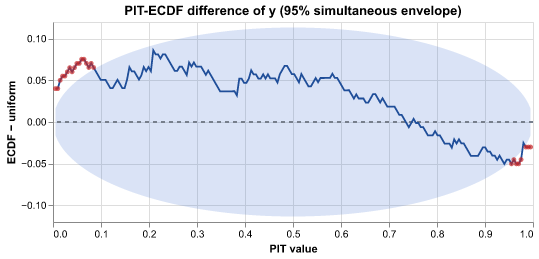
How to read it. The line goes above the band near 0 and below it near 1: too many actual values are in the tails. The predicted ranges of the model are too narrow.

Use it when

• You want a sharper check of the predicted ranges than the PIT histogram
• You predict a yes/no outcome and want to know if a 70% prediction comes true about 70% of the time
• You fitted a classifier that gives one probability for each row, without draws

Avoid it when

• You have no actual values to compare with
• You have only a few observations (fewer than about 30)

What it needs

• Predictions with draws (posterior_predictive or predictions group), or one predicted probability for each cell for a yes/no outcome
• The actual values (observed_data or observed group)

What is on the chart

• For numbers: the PIT-ECDF difference with a 95% band that holds at all points together
• For yes/no outcomes: a reliability diagram with a band for each group and a histogram of the predicted probabilities
• Red points where the line or a group is outside its band
• A caption with the verdict, and the Brier score for yes/no outcomes

For experts

Continuous: PIT = P(ŷ < y) + ½ P(ŷ = y); the line is ECDF(z) − z on a grid of min(max(n, 20), 200) points. The simultaneous envelope at prob (0.95) is ±c·sqrt(z(1−z)/n) with c the prob quantile of the largest standardised deviation over the grid in n_sim (1000) simulated uniform samples (cumulative multinomial counts, seed). Binary (auto when y ∈ {0, 1} and the draws are in [0, 1]): bins (10) equal-width bins of the mean prediction; each band is the binomial range p ± z·sqrt(p(1−p)/n_bin); the expected calibration error weights |observed − predicted| by bin size. A point prediction (no sample dims, values in [0, 1], for example the y_hat of an sklearn classifier) takes the binary path with the probability as the mean; var and observed_var pick the pair. A point prediction of a target that is not 0/1 is an error, because the PIT check needs draws.

Confusion matrix

core.confusion@1.0.0

Counts the cases that the model classifies correctly and incorrectly, for a binary or multiclass target. For yes/no, the four boxes are the true and false positives and the true and false negatives at one probability threshold.

How to read it. At the threshold 0.5, the model finds 62 of the 80 positive cases (recall 0.78). 25 of its 87 alarms are false (precision 0.71). With the threshold auto, the threshold goes down to 0.31. The recall goes up to 0.9 and the precision goes down to 0.6.

Use it when

• You must change the probabilities into yes/no decisions and want to see the errors
• You want the precision, the recall and the specificity at one threshold
• You want to explain the errors of a classifier to people who do not read models

Avoid it when

• You want to see all thresholds (use ROC and precision-recall curves)

What it needs

• Predicted probabilities of the positive class, with draws or one value for each cell (posterior_predictive, predictions or draws group, or a score summary)
• The actual 0/1 values (observed_data or observed group)

What is on the chart

• A 2 × 2 matrix of the actual class against the predicted class, with counts or with the share of each actual class
• For a multiclass target: a K × K matrix of the most probable class (up to 30 classes; the other classes are put together), with the accuracy and the macro F1
• A caption with the accuracy, the precision, the recall (sensitivity), the specificity, the F1 score and the threshold

For experts

threshold is a number (default 0.5) or 'auto': the threshold that maximises Youden's J = TPR − FPR over the distinct predicted probabilities. normalize='true' divides each row (actual class) by its count; 'none' shows counts. Precision = TP/(TP+FP), recall = TP/(TP+FN), specificity = TN/(TN+FP), F1 = 2PR/(P+R). positive, var and observed_var work as in ROC and precision-recall curves. Multiclass: the predicted class is the argmax of the class probabilities; threshold and positive are not used (the caption says so).

Sampler convergence

core.convergence@1.0.0

Checks that the fitting method found stable answers for each model parameter. Red points and a 'check' status show the parameters that you must not trust yet.

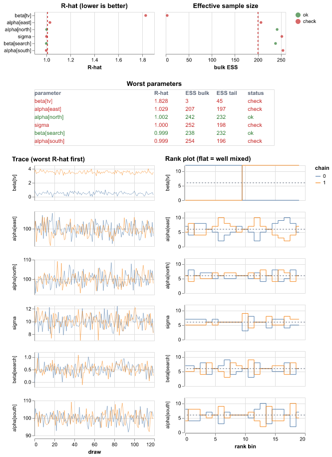
How to read it. beta[tv] has R-hat 1.8 and its two trace lines stay at different levels: the chains disagree. The rank plot is not flat. Run the sampler longer or change the model before you use beta[tv]. The caption also reports 3 divergent transitions.

Use it when

• You fitted a Bayesian model and want to know if you can use it
• Results change from run to run

Avoid it when

• The model is not fitted with draws (such as a least-squares model)
• You want to know if the model is correct (a converged model can still be wrong)

What it needs

• A fitted Bayesian model with draws in chains (the posterior group)
• Optional: sample_stats with the divergence flags

What is on the chart

• A dot for R-hat of each parameter with a red limit line
• A dot for the effective sample size of each parameter with a limit line
• A table of the worst parameters
• Trace lines and rank plots of the worst parameters
• A caption with the number of problems and divergent transitions

For experts

Rank-normalised split R-hat (max of bulk and folded), bulk and tail ESS, per parameter element. A row is 'check' when R-hat > rhat_threshold (default 1.01) or min(bulk, tail ESS) < ess_per_chain × chains (default 100 per chain). Sorted by R-hat; max_parameters (40) dots, table_rows (15) table rows, max_traces (6) traces and rank histograms (bins, default 20; flat = well mixed). max_elements (2000) caps the elements checked. Divergences come from sample_stats.diverging.

Scenario vs baseline

core.counterfactual@1.0.0

Compares a 'what if' scenario with the baseline over time. It also shows how sure the model is about the total difference.

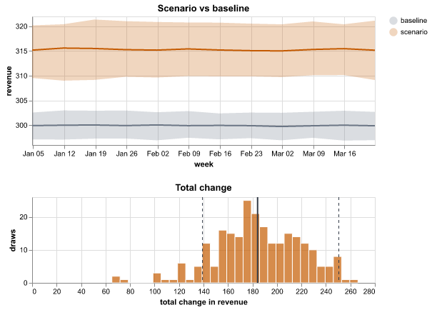
How to read it. The scenario line is above the baseline every week. The histogram of the total change is from 40 to 80, all above zero. The caption says that the probability of an increase is 100%.

Use it when

• You changed an input, such as spend or price, and want to see the effect
• You want the probability that the scenario does better

Avoid it when

• You compare more than one scenario (use Decision outcome)
• The scenario is far outside the data that the model saw

What it needs

• A scenario score: scenario draws (or summary) and baseline draws (or summary)
• Optional: delta draws (scenario minus baseline) for the total difference

What is on the chart

• Two lines with 90% bands: the scenario and the baseline
• A histogram of the total change, with its mean and a 90% range
• A caption with the change and the probability of an increase

For experts

Bands are equal-tailed quantiles of the draws summed over hidden dims; summary inputs use their interval statistics. The total change sums the delta draws over all dims (or scenario − baseline when both have draws); the histogram uses bins (default 30) and the range is an HDI at hdi_prob. When only summaries exist, the chart shows the difference of the means with no uncertainty.

Data overview

core.data_overview@1.0.0

Shows each column of your data over time, where values are missing and how much data each group has. Use it before you fit a model.

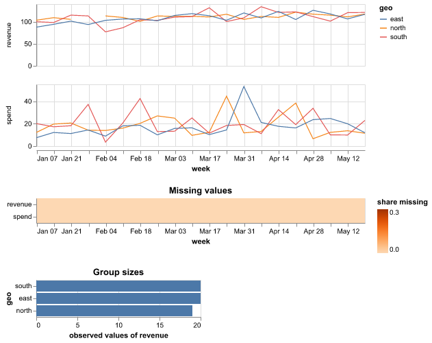
How to read it. The revenue panel has a gap in week 4 for 'north'. The heatmap shows that search spend is missing for the first four weeks in 'east'. Fix or fill these values before you fit the model.

Use it when

• You uploaded a dataset and want a first look
• You want to find gaps, spikes or groups with little data

Avoid it when

• Your data has no numeric columns
• You want a plot of model results

What it needs

• A dataset, or the observed_data, data or constant_data group of a run

What is on the chart

• One panel for each column with a line for each group
• A heatmap of the share of missing values over time
• Bars of the number of values in each group
• A caption with the column that has most missing values

For experts

The time dim is detected (or along); the colour dim is a small categorical dim (facet, at most max_levels levels). Other dims are summed with min_count=1. The heatmap is the mean of isnull() over the other dims. Group sizes count non-null values of the first variable. vars and max_vars pick columns; above max_rows the x values are thinned evenly.

Decision outcome

core.decision_distribution@1.0.0

Shows the range of results for each option of a decision. It also gives the probability that each option is the best.

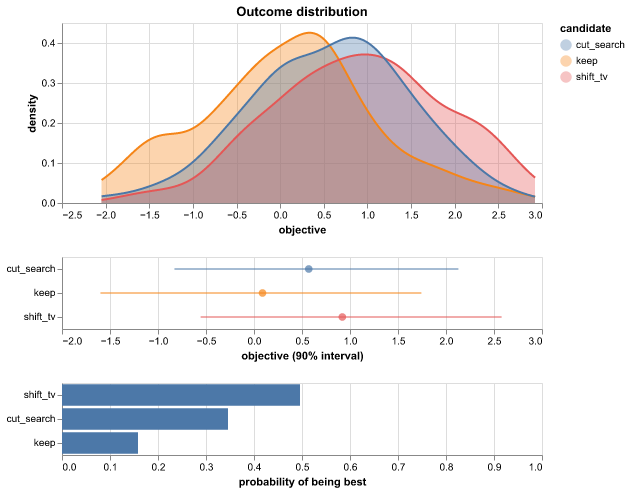
How to read it. 'shift_tv' has the highest curve and a 64% probability to be the best. Its range overlaps with 'cut_search', so the choice is not certain. 'keep' is best in only 8% of the draws.

Use it when

• You choose between a few options, such as budget splits
• You want to see the risk of each option, not only its average

Avoid it when

• The result has more than one value for each option (sum it first)
• You have no draws, only averages

What it needs

• A decision group with draws of one result for each option (an option dimension)

What is on the chart

• Smooth curves of the results of each option
• A dot and a 90% range for each option
• Bars of the probability that each option is the best
• A caption that names the best option

For experts

Needs sample draws (chain/draw or sample). Densities are KDEs on a shared grid from the 0.5th to the 99.5th percentile; ranges are HDIs at hdi_prob. P(best) is the share of draws where the option has the highest (or lowest, with higher_is_better false) value, which needs the options to share draws. candidate names the option dim (default: the only extra dim); max_candidates caps it at 12.

Decomposition

core.decomposition@1.0.0

Splits the outcome into the parts that the model adds together, such as a baseline and each driver. It shows each part over time and its total share.

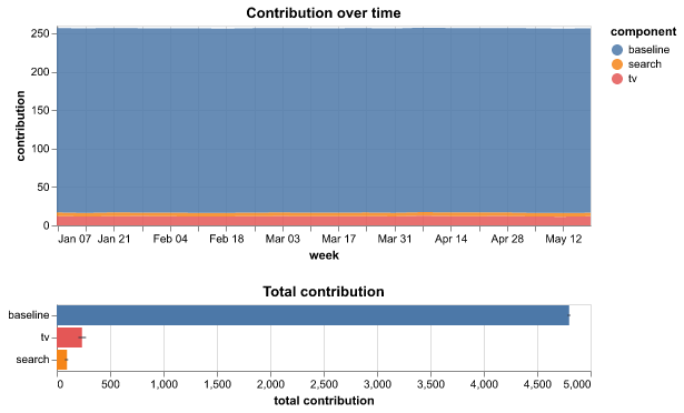
How to read it. The baseline gives 85% of revenue, TV 10% and search 5%. The 90% range of search includes zero, so the model is not sure that search adds anything.

Use it when

• You want to know how much each part of the model explains
• You want to explain the result to people who do not read models

Avoid it when

• Your model does not add its parts together
• Some parts are negative and large (a stacked area is then hard to read)

What it needs

• A contributions, decomposition or components group with one variable or label for each part, over time

What is on the chart

• Stacked areas of each part over time
• Bars of the total contribution of each part with a 90% range
• A caption with the share of the top parts, and the parts that can be zero

For experts

Components are the labels of a component dim (component, default the first of component/channel/contribution/term/effect) plus whole variables without it. The area uses the mean over draws per time; the bar uses the mean of each draw's total with an HDI at hdi_prob (default 0.9). Shares are of the summed means. max_components caps the parts (default 20). Groups: contributions, decomposition, then components (the unobserved-components and ETS states, the HSGP trend and seasonality). A variable with attr decomposition='exclude' (the UC and ETS slope state, which is a rate and not an additive part) is skipped unless vars names it.

Sampler energy

core.energy@1.0.0

Checks if the fitting method can move through all of the possible values of the model, including the extreme ones. A red bar shows a chain with a problem.

How to read it. The E-BFMI of chain 1 is 0.19, below 0.3. The blue histogram is much narrower than the grey one. The sampler does not reach the tails, so make the priors narrower or change the parameterisation.

Use it when

• You fitted a Bayesian model with NUTS or HMC and want to check the sampler
• The convergence check is good, but you do not trust the extreme values

Avoid it when

• The model is not fitted with NUTS or HMC (there is no energy)
• You want to know if the model is correct

What it needs

• A sample_stats group with the energy of each draw in each chain

What is on the chart

• Two histograms: the energy (grey) and its change from one draw to the next (blue)
• A bar for the E-BFMI of each chain with a dashed limit line
• A caption that names the chains below the limit

For experts

E-BFMI per chain = mean(diff(E)²) / var(E) (ArviZ bfmi, Betancourt 2016). The histograms pool the chains: marginal energy E − mean(E) per chain, transitions diff(E) − its mean per chain, on shared bins (40) between the 0.5% and 99.5% points. bfmi_threshold (0.3) sets the limit.

Predicted vs actual

core.fit_vs_actual@1.0.0

Puts each prediction of the model next to the actual value in a scatter plot. Dots on the dashed diagonal line are perfect predictions.

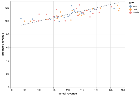
How to read it. Most dots are near the diagonal and the caption says R² = 0.85. The dots for 'south' are all below the line, so the model predicts too low for that market.

Use it when

• You want a quick view of how accurate the model is
• You want to find the cells where the model is far wrong
• Your data has no time dimension

Avoid it when

• You want to see when the errors happen (use Residuals over time)
• You need to see the range of the predictions (this chart shows only the middle value)

What it needs

• Predictions with draws (posterior_predictive, predictions or draws group), or a score summary with interval statistics
• The actual values (observed_data or observed group)

What is on the chart

• A dot for each cell: the actual value across, the prediction up
• A dashed diagonal line for perfect predictions
• Colours for each market or product when there is a group dimension
• A caption with R² and the typical error in percent (MAPE)

For experts

Point = median or mean of the draws (or the summary's point statistic). With draws, hidden dims are summed; with a score summary, the extra dims are kept as cells. R² = 1 − SS_res / SS_tot on the plotted cells (not a held-out score). MAPE skips cells where the actual value is zero. The chart is the same for train and test cells: filter the input to judge the forecast.

LOO-PIT and Pareto k

core.loo_pit@1.0.0

Checks each actual value against the predictions of the model when that value is left out of the fit. It also finds the values that have too much effect for this check to be reliable.

How to read it. 3 of 120 values (2.5%) have a Pareto k of more than 0.7. All three are in the week of the holiday sale, which the model does not know about. The PIT line stays in the band, so the other predictions are well calibrated.

Use it when

• You want a calibration check that does not use each actual value two times (one time to fit and one time to check)
• You want to find values that have a large effect on the model, such as outliers
• You want to know if you can trust the LOO score (elpd_loo) of a model

Avoid it when

• The model has no log_likelihood group
• The model gives only one value for each cell, with no draws

What it needs

• Draws with a log_likelihood group
• For the PIT panel: posterior_predictive draws and the actual values (observed_data group)

What is on the chart

• The LOO-PIT ECDF difference with a 95% band that holds at all points together (when the posterior_predictive and observed_data groups are present)
• A dot for the Pareto k of each value, coloured good (less than 0.5), ok or bad (more than the threshold), with lines at 0.5 and at the threshold
• A caption with the number and the share of values above the threshold, and the verdict on the PIT line

For experts

PSIS (Vehtari et al. 2024) on the log ratios −log p(y_i | θ_s): tail length M = ceil(min(0.2 S, 3 √S)), a generalized Pareto fit (Zhang and Stephens, with the weakly informative prior) whose quantiles replace the tail, truncated at the largest raw weight; k = inf when the tail is too short. LOO-PIT_i = Σ_s w_si 1[ŷ_si < y_i] + ½ Σ_s w_si 1[ŷ_si = y_i] with the normalised weights. The envelope is the simultaneous one of Calibration (prob 0.95, n_sim 1000, seed). Draws are thinned evenly to max_draws (2000). var picks the log_likelihood variable (default: the first), observed_var the actual values; k_threshold (0.7) sets the bad line. The bundle's metrics.json also keeps the k of elpd_loo (pareto_k).

Training loss

core.loss_curve@1.0.0

Shows the loss of a fit that runs in steps, such as ADVI, at each step. A flat curve at the end shows that more steps will not make the fit better.

How to read it. The moving average goes from 12 400 to 830. Over the last 10% of the steps, it goes down by 4% more. The loss still goes down at the end, so more steps can make the fit better.

Use it when

• You fitted a model with ADVI and want to know if it had sufficient steps
• You want to compare the training loss and the validation loss of a model that records both

Avoid it when

• The model was fitted with MCMC (use Convergence)
• The run did not record a loss at each step

What it needs

• A fit_history group (an ADVI fit writes it) or a metrics_history group, with one variable for each curve over a step dimension

What is on the chart

• The raw loss as a light line
• A moving average as a dark line
• A log scale when all values are more than zero and the largest value is more than 50 times the smallest value
• A caption with the first and the last value of the moving average and its change over the last 10% of the steps

For experts

group='auto' takes fit_history, then metrics_history; var picks one variable; along is the step dim (default 'step'). The smoothed line is a rolling mean with window smooth (default max(1, n // 50)). log_y=None uses log10 when all values > 0 and max/min > 50. Up to max_points (2000) evenly spaced steps, the last step always kept. The ADVI history keeps at most 5000 evenly spaced steps (the dataset attr thinned_from holds the original count). The caption warns when the smoothed loss still falls by more than 1% over the last 10% of the steps. The run adds this plot to every fit with a fit_history group.

Model comparison

core.model_comparison@1.0.0

Ranks two or more models by how well they are expected to predict new data. It shows how far each model is from the best one and how sure that difference is.

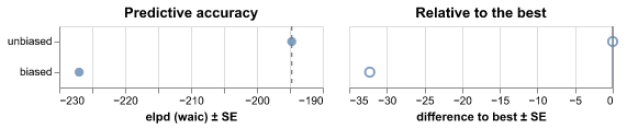
How to read it. 'unbiased' is best. 'biased' is 35 ± 6 elpd worse. That is more than twice the standard error, so the difference is clear. Use 'unbiased'.

Use it when

• You fitted more than one model to the same data and want to pick one
• You want to know if a more complex model is worth it

Avoid it when

• The models use different data or a different outcome
• You have only one model

What it needs

• A comparison group (for example from PSIS-LOO), or the log_likelihood group of each model

What is on the chart

• A dot and a ±1 standard error line for the score (elpd) of each model
• A dot and a ±1 standard error line for the difference to the best model
• A caption that names the best model and judges the gap

For experts

With ic='auto' a precomputed comparison group (elpd/elpd_loo/elpd_waic/elpd_kfold, se, dse, weight on a model_dim) is used as is; otherwise WAIC is computed from each child's log_likelihood (var picks the variable) and dse = sqrt(n · var(pointwise difference)) to the best model. Verdict on the runner-up: |Δelpd| < 4 is very small; > 2 dse is clear; else smaller than its uncertainty. Prefer PSIS-LOO over WAIC when it is available.

Pair plot

core.pair@1.0.0

Shows the draws of each pair of model parameters as a cloud of points, with a histogram of each parameter. Red points mark draws where the fitting method had problems.

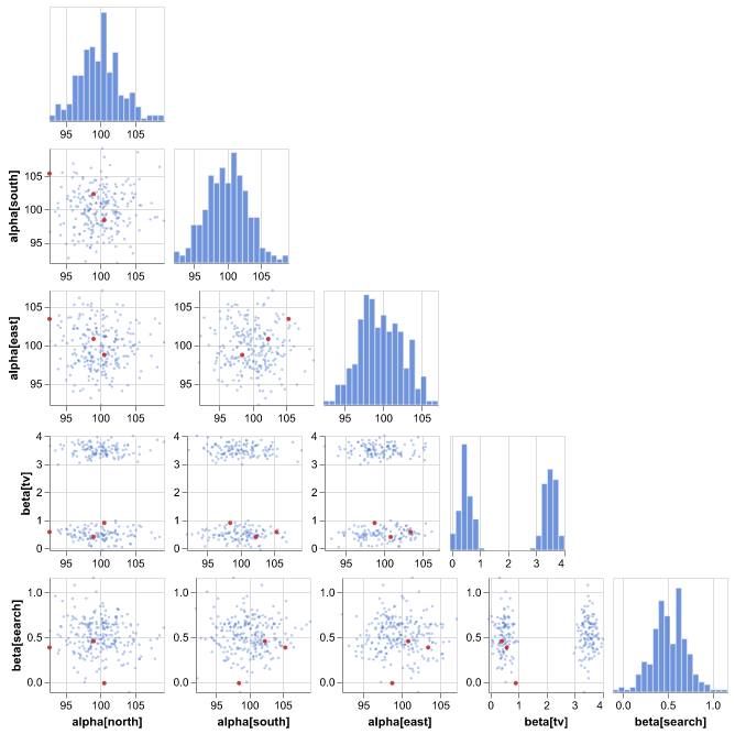
How to read it. The cloud of beta[tv] against alpha[north] has two separate groups of points: the two chains found different values of beta[tv]. The 3 red points are inside the clouds, so they do not point to a funnel.

Use it when

• Sampler convergence reports divergent transitions and you want to see where they are
• You want to see if two parameters trade off against each other
• You want to see the shape of the fitted values, such as two peaks or a funnel

Avoid it when

• The model has many parameters and you do not know which ones to look at
• You want the ranges of many parameters at once (use Posterior forest)

What it needs

• A fitted Bayesian model with draws in chains (the posterior group)
• Optional: sample_stats with the divergence flags

What is on the chart

• A histogram of each parameter on the diagonal
• A cloud of points for each pair of parameters below the diagonal
• Red points for the divergent transitions
• A caption with the strongest correlation and the number of divergences

For experts

Elements of var_names (default: every numeric posterior variable) are taken in model order up to max_params (5; constant elements are skipped). The scatters show up to max_draws (500) evenly thinned draws plus the divergent draws; the histograms (bins, 20) use all draws. Each axis spans the full range of the draws. Divergences come from sample_stats.diverging when its (chain, draw) shape matches. The caption reports the largest |Pearson r| over all draws; above 0.8 it suggests a reparameterisation.

Posterior forest

core.posterior_forest@1.0.0

Shows the estimate and the range of each model parameter as a row with a dot and two lines. Rows whose range does not include zero have a clear direction.

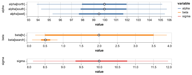
How to read it. beta[tv] is 0.5 with a 94% range from 0.1 to 0.9: the effect is clearly positive. beta[search] goes from −0.2 to 0.6, so its direction is not certain.

Use it when

• You want to read the fitted values of the parameters
• You want to see which effects are clearly positive or negative

Avoid it when

• The parameters have no clear meaning on their own (for example, many latent values)
• The fit has not converged (check Sampler convergence first)

What it needs

• A fitted Bayesian model with draws (the posterior group)

What is on the chart

• A dot for the median (or mean) of each parameter
• A thick bar for the middle 50% range
• A thin line for the 94% range
• A dashed zero line for variables whose ranges cross zero
• One panel with its own scale for each variable

For experts

The thin line is the HDI at hdi_prob (default 0.94, the ArviZ default); the thick bar is the central (equal-tailed) interval at inner_prob (default 0.5). point is median or mean. Elements are listed in model order up to max_rows (60); var_names picks variables. The caption counts intervals that exclude zero, which only matters for parameters where zero means 'no effect'.

Posterior predictive check

core.ppc@1.0.0

Compares data that the fitted model makes with your actual data. It shows if the ranges of the model are too narrow, too wide or shifted.

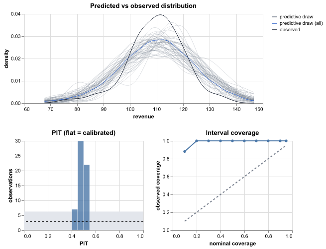
How to read it. The coverage line is below the diagonal and only 70% of the values are in the 90% range. The PIT histogram is high at both ends (a U shape). The ranges of the model are too narrow, so the model is too sure.

Use it when

• You want to check if the model's ranges are honest
• You want to see if the model gets the shape of the data right, such as its tails

Avoid it when

• You want to see the fit over time (use Fit and forecast)
• You have no draws, only averages

What it needs

• Predictions with draws (the posterior_predictive group)
• The actual values (observed_data group)

What is on the chart

• Thin curves for the shape of some predicted datasets and a dark curve for your data
• A PIT histogram with a grey band for the expected count (flat = calibrated)
• A coverage line against the ideal diagonal
• A caption with the coverage of the 90% range and warnings

For experts

PIT = P(ŷ < y) + ½ P(ŷ = y) per observed cell over the matched draws. The PIT histogram uses bins (default 20) and a ±1.96 SD binomial band. Coverage is the share of observations inside central equal-tailed intervals at levels (0.1 to 0.95). Caption rules: mean PIT < 0.4 (over-predicts) or > 0.6 (under-predicts); > 20% of PIT values in the outer 10% (too narrow); < 2% with n ≥ 50 (too wide). PIT values are not independent across time, so treat the band as a guide.

Fit and forecast

core.ppc_fan@1.0.0

Shows the model's estimate over time as a line with shaded ranges, and the actual values as dots. A dashed line marks where the training data ends and the forecast starts.

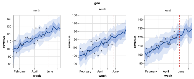
How to read it. The 90% band covers 18 of the 20 actual weeks and the line goes through the dots: the model fits the history well. After the dashed line, three weeks in a row are above the band. The model probably missed a change in level at that time.

Use it when

• You want to see how well the model follows the history
• You want to show a forecast with its range to other people
• You want to check the forecast against values that the model did not see

Avoid it when

• Your data has no time or order dimension
• You want to compare single predictions with actual values cell by cell (use Predicted vs actual)

What it needs

• Predictions with draws (posterior_predictive, predictions or draws group), or a score summary with interval statistics
• Optional: the actual values (observed_data or observed group)
• A time-like dimension, such as week or date

What is on the chart

• A line for the median (or mean) estimate
• Shaded 50% and 90% bands
• Dots for the actual values
• A dashed line where the training data ends
• One panel for each market or product when the data has a small group dimension
• A caption with the share of later actual values inside the 90% band

For experts

Bands are per-time quantiles of the draws (equal-tailed, at levels, default [0.5, 0.9]) after summing the draws over the hidden dims; joint draws make totals valid. A score summary uses its hdi_/eti_/q* statistics and cannot be summed. point picks median or mean. split_at sets the dashed line (default: the tree attr split_at, else the first x after the last observation). facet and max_facets pick the panel dim; the y axes are independent per panel. The caption's coverage counts only observations after the split, in the widest band.

Prior and posterior

core.prior_posterior@1.0.0

Shows, for each parameter, the values that the model allowed before it saw the data and the values after the fit. Parameters that the data moved most come first.

How to read it. beta[tv] moved most: its mean changed by 2.2 prior standard deviations. The prior and the posterior of sigma overlap by 21%, so the data told the model much about the noise. A parameter with 90% overlap depends mostly on its prior.

Use it when

• You want to know what the data taught the model
• You want to find parameters that only the prior controls
• You want to check that a prior is not too narrow

Avoid it when

• The model has no prior group
• The model has hundreds of parameters (the chart shows the top ones only)

What it needs

• A prior group and a posterior group with draws of the same variables

What is on the chart

• One panel for each parameter with the prior (grey) and the posterior (blue)
• Panels sorted by how far the mean moved, in prior standard deviations
• A caption with the overlap of each pair and the parameters where the data adds little

For experts

Variables in both groups with draws (or var_names). Per cell: Gaussian KDE (Silverman) of prior and posterior on a shared grid of points (80); overlap = ∫ min(p, q). Cells are ranked by |mean_post − mean_prior| / sd_prior; at most max_cells (8) per variable and max_vars (12) variables. Overlap above little (0.8) is reported as 'the data adds little'.

Prior predictive check

core.prior_predictive@1.0.0

Shows data that the model can make before it sees your data, next to your data. Use it to check that your starting assumptions give values of the right size.

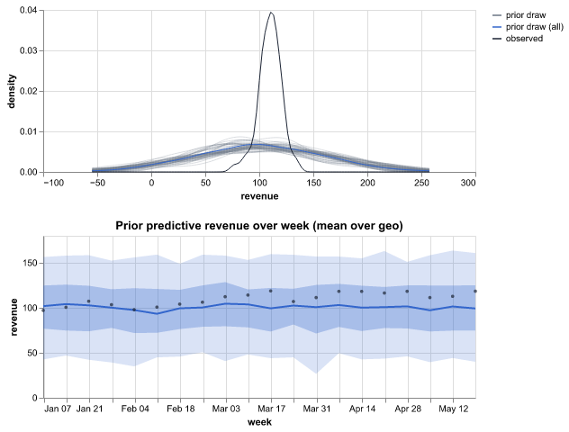
How to read it. The grey curves spread from −100 to 300 and your weekly revenue is between 80 and 130. 100% of your values are inside the 90% range, so the beliefs allow the data. If the curves went to 10 000, the beliefs would be much too wide.

Use it when

• You set the starting beliefs of a Bayesian model and want to check them
• The fit fails or is slow and you suspect the starting beliefs

Avoid it when

• The model is not Bayesian
• You want to judge the fitted model (use Posterior predictive check)

What it needs

• A prior_predictive group (draws of the outcome before fitting)
• Optional: the actual values (observed_data group) with the same variable name

What is on the chart

• Thin grey curves: the shape of the data in some draws
• A thick blue curve for all draws together
• A dark curve for your data
• A band over time when the data has a time dimension
• A caption with the share of your values inside the 90% range

For experts

Densities are KDEs of num_draws (default 50) evenly spaced prior predictive draws plus the pooled draws. Over time: quantile bands at levels of the mean over the other dims. The caption counts observations inside the per-cell 90% equal-tailed interval; under 50% suggests priors too narrow or on the wrong scale, and a median width over 100 × the data range suggests priors too wide. The observed variable must have the same name as the predicted one.

Rank matrix

core.rank_matrix@1.0.0

Shows how likely each item is to have each place in a ranking, and how likely each item is to be above each other item. Use it when the order of items matters more than their values.

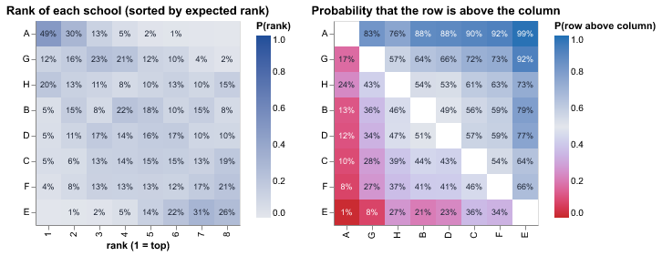
How to read it. School A is first in 49% of the draws and is above school G in 83% of them. The middle schools have spread-out rows: their places are not certain.

Use it when

• You want to rank teams, products, schools or regions and know how sure the ranking is
• You want the chance that one item is better than another

Avoid it when

• There are more than 30 items (raise max_items to 60 at most)
• Ties are common and meaningful (the chart breaks ties in a fixed order)

What it needs

• Draws of a variable with one item dimension, in the posterior, predictions or posterior_predictive group

What is on the chart

• A heatmap of the chance of each rank for each item, sorted by the expected rank
• A heatmap of the chance that the row item is above the column item
• Percentages in the cells when there are 12 items or fewer
• A caption with the top item and how sure its place is

For experts

Per draw, items are ranked by value (descending: rank 1 = largest; ties keep item order). P(rank = k) is the share of draws, the expected rank sorts the rows, and P(row above column) = P(x_row > x_col) for descending (else <). Up to max_draws (4000) draws with every item finite; max_items (30) items. labels (auto: at most 12 items) prints the percentages.

Residuals over time

core.residuals_over_time@1.0.0

Shows the error of the model (actual minus predicted) for each point in time. The errors should stay near the zero line with no pattern.

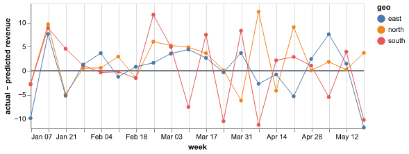
How to read it. The residuals stay between −10 and +10 until June, and then they are all above zero. The model under-predicts from June, so it probably misses a change in the level or a new driver.

Use it when

• You want to find structure that the model does not capture
• You suspect a trend, a season or a one-time event that the model misses

Avoid it when

• You need a first view of the fit (start with Fit and forecast)
• You have very few time points

What it needs

• Predictions with draws (posterior_predictive, predictions or draws group), or a score summary with interval statistics
• The actual values (observed_data or observed group)

What is on the chart

• A line with points for the residual at each time
• A zero line
• One colour for each market or product when there is a group dimension
• A caption that says if the model is too high or too low on average

For experts

Residual = observed − point (median or mean), on the same cells as Predicted vs actual. The caption reports an average bias when |mean residual| > 5% of the mean |observed|. Look for runs on one side of zero (bias over time), waves (a missing season), a funnel (spread that grows with the level) and single spikes (events or data errors).

Ridgeline

core.ridge@1.0.0

Shows a curve of the possible values for each group, such as each school or each region, one above the other and sorted by the average. Use it to compare many groups at once.

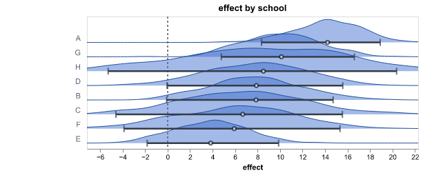
How to read it. School A is at the top with a mean effect of 14 and school E is at the bottom with 4. The bars of most neighbouring schools overlap, so only the difference between the top and the bottom is clear.

Use it when

• Your model has one value for each group and you want to compare the groups
• You want to see the shape of each range, not only its ends

Avoid it when

• There are more than 30 groups. The chart then shows only 30 of them (raise max_levels to 100, or use Posterior forest)
• The variable has more than one dimension that you cannot fix to one level

What it needs

• Draws of a variable with one group dimension, in the posterior, predictions or posterior_predictive group

What is on the chart

• One smoothed curve for each group, sorted by the mean
• A dot for the mean and a bar for the 94% range of each group
• A dashed zero line when the values cross zero
• A caption with the top and bottom groups and how many neighbours overlap

For experts

Gaussian KDE (Silverman bandwidth) per level on a common grid over the 0.5–99.5 % range of all draws (points, 100), each scaled so its peak is overlap (1.6) row heights. Bars are the HDI at hdi_prob (0.94). Rows are ordered by mean (descending puts the largest on top); above max_levels (30), evenly spaced rows in that order are kept. dim picks the level dim when the variable has more than one; select fixes the others. Up to max_draws (4000) draws.

ROC and precision-recall curves

core.roc_pr@1.0.0

Shows how well the predicted probabilities separate the yes cases from the no cases at all thresholds, for a binary or multiclass target. A curve near the top-left corner (ROC) or the top-right corner (precision-recall) shows a good separation.

How to read it. The AUC is 0.86, so the model separates the classes well. Only 8% of the cases are positive. The precision falls below 0.5 when the recall is more than 0.6. At that point, half of the alarms are false.

Use it when

• You predict a yes/no outcome and want one number for how well the model puts the cases in order
• You want to see the balance between the cases that the model finds and its false alarms at all thresholds
• The yes cases are rare. The precision-recall curve shows this better than the ROC curve
• You classify into three or more classes and want a curve for each class

Avoid it when

• You want to know if the probabilities are correct (use Calibration)
• You need the result at one threshold (use Confusion matrix)

What it needs

• Predicted probabilities of the positive class, with draws or one value for each cell (posterior_predictive, predictions or draws group, or a score summary)
• The actual 0/1 values (observed_data or observed group)
• For a multiclass target: the probability of each class along a class dim, and the actual class labels

What is on the chart

• The ROC curve: the true positive rate against the false positive rate, with a diagonal line for a random guess
• The precision-recall curve, with a line at the base rate (the share of positive cases)
• The AUC and the average precision in the titles of the panels
• A caption with a verdict on the AUC and the base rate. With draws, the caption also gives a 90% range of the AUC
• For a multiclass target: one curve for each class against all other classes (the 12 most frequent classes), and the macro AUC in the title

For experts

The thresholds are the distinct predicted probabilities, thinned to max_points (500, 20..5000). The AUC is the Mann-Whitney statistic with average ranks for ties. The average precision summarises the precision-recall curve. With draws, the AUC of each draw (up to 500 draws) gives the 90% interval in the caption. Verdict on the AUC: >= 0.9 very well, >= 0.8 well, >= 0.7 fairly well, else not well. positive picks the value of the positive class (default: the larger one); var and observed_var pick the pair. On imbalanced data, read the precision-recall panel: the ROC curve can look good while most alarms are false. Multiclass (a class dim on the prediction, or more than two observed classes): one-vs-rest curves per class, the macro AUC is the mean over the classes, classes picks the classes to draw and positive is not used.

State sequence

core.state_sequence@1.0.0

Shows your data over time above the probability of each hidden state, such as a calm or a busy period. Use it to see when the state changes and how sure the model is.

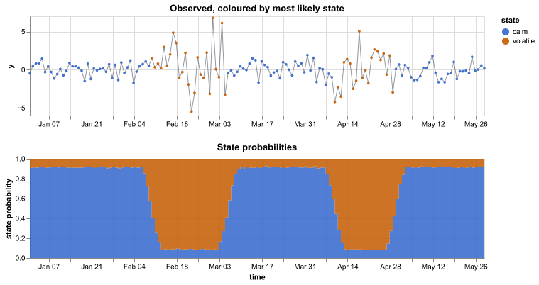
How to read it. The volatile state has a high probability from mid-February to early March and in late April. The large swings in the data are at the same times. At the edges of these periods neither state reaches 80%, so the exact change dates are not certain.

Use it when

• Your model has hidden states or regimes, such as a hidden Markov model
• You want to find change points in a series

Avoid it when

• The states have no fixed labels between draws (label switching). Fix the order in the model first
• There are more than about 10 states

What it needs

• State probabilities with a state (or regime) and a time dimension, or draws of the state number at each time. The chart looks in the hidden_states, regimes, posterior, predictions, posterior_predictive and summary groups
• Optional: the observed series (observed_data group)

What is on the chart

• The observed series with each point coloured by its most likely state
• Stacked areas of the probability of each state at each time
• A caption with the number of changes, the share of time in each state and the times with no clear state

For experts

group='auto' looks in hidden_states (HMM), regimes (Markov switching), posterior, predictions, posterior_predictive, summary, then the root. var defaults to smoothed_prob, state_prob or filtered_prob, else a numeric variable with a state dim and one more dim (so transition and expected_duration are skipped), else integer state draws. state_dim='auto' takes 'state', then 'regime', then a dim whose name contains either. A probability variable is the mean over draws (up to max_draws), clipped at 0 and normalised at each time; a score summary uses its stat='mean' row (else median, else point). Integer state draws are counted per time. along sets the time dim. Without select, every other dim with more than one level is fixed at its first level and the caption names it; with select, a missing level is an error. observed_var picks the series (default: the first observed variable with the time dim); NaN padding is dropped. The most likely state colours the points; up to max_times (2000) evenly spaced times.

Confusion over epochs

ml.confusion_epochs@1.0.0

Shows the confusion matrix of the validation data at some epochs of the training. You can see which classes the network learns first and which classes it confuses to the end.

How to read it. At epoch 1 the network puts most images in the class 'can'. At the best epoch (12), the accuracy is 0.91. The network still confuses only 'bottle' and 'jar'.

Use it when

• You trained an image or table classifier and want to see how the errors changed
• Some classes stay hard and you want to know which classes the network confuses

Avoid it when

• The model has no validation data or was not trained in epochs (use the confusion matrix)

What it needs

• A training group with confusion(epoch, true_class, pred_class) counts (the mapi-jax classifiers write it)

What is on the chart

• Up to 6 small matrices: the first epoch, some epochs between, the best epoch and the last epoch
• Each row is shown as a share of its actual class, or as counts
• A caption with the validation accuracy at the first, the best and the last epoch

For experts

epochs picks the epochs (default: first, evenly spaced, best and last, at most 6); normalize is 'true' (rows divided by the actual-class count) or 'none'; max_classes keeps the most frequent classes and pools the rest.

Feature importance

ml.feature_importance@1.0.0

Ranks the inputs that a tabular model uses most. For a linear model it shows the size and the direction of each input's effect.

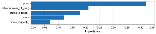
How to read it. price has 42% of the total importance and the week of the year has 21%. promo_lagged[2] has 7%, so the second week after a promotion adds little. For the linear model, the price coefficient is −1.8: a higher price lowers the prediction.

Use it when

• You want to know which inputs drive the predictions
• You want to find inputs that the model ignores

Avoid it when

• You want cause and effect (importance shows use, not cause)
• Inputs are strongly related, so the model can use either one

What it needs

• A feature_importance group from a tree model, or a coefficients group from a linear model

What is on the chart

• Bars for each input, largest first (at most 20)
• Red bars for negative coefficients and blue bars for positive ones
• A range line when there are several models (such as one for each quantile)
• A caption that names the top input and its share

For experts

source='auto' uses the feature_importance group, else coefficients; groups are found at the root, under model/ or anywhere in the tree. Coefficients are ranked by |value|. Extra dims (for example one model per quantile) give the mean as the bar and min to max as the range line. top (default 20) caps the bars; feature_dim names the feature dim. Permutation importance or SHAP is more reliable than impurity importance.

Wrong validation images

ml.misclassified@1.0.0

Shows the validation images that the network classifies incorrectly, with the true class, the predicted class and its probability. Look at them to find wrong labels or classes that look the same.

How to read it. 37 of 400 validation images are wrong at epoch 12. Five 'cat' images that the network calls 'dog' with p = 0.97 have a dog in them: their labels are wrong.

Use it when

• You trained an image classifier and want to see its errors
• You think that some labels are wrong

Avoid it when

• The data are not images
• The model has no validation images

What it needs

• A misclassified group with small images and their true and predicted labels (the mapi-jax image classifiers write it)

What is on the chart

• A grid of up to 24 small images
• Above each image: true class → predicted class and the probability
• A caption with the number of wrong images and of validation images

For experts

Plotly image traces with z pixel arrays (RGB uint8; gray images repeat to three channels; no source URLs). max_items (default 24) and columns (default 6) set the grid. The images are sorted by the predicted-class probability, highest first.

Training and validation curves

ml.training_curves@1.0.0

Shows the loss and the accuracy of a neural network on the training data and on the validation data while it learns. When the validation loss goes up and the training loss goes down, the network starts to overfit.

How to read it. The validation loss is lowest at epoch 7 (0.41). After epoch 9 it goes up while the training loss goes down, so the network starts to overfit. Early stopping kept the weights of epoch 7.

Use it when

• You trained a network and want to know if it had sufficient epochs
• You want to see when the network started to overfit and which epoch was the best

Avoid it when

• The model was not trained in steps (use Convergence or the scorecard)

What it needs

• A metrics_history group with a split label (train and val), or a training group with train_* and val_* variables for each epoch

What is on the chart

• One panel for each metric (loss, accuracy or error, up to 4), with one line for each split
• Points on the validation line
• A caption with the best validation value and its step or epoch, and a note when the network starts to overfit

For experts

Reads metrics_history (per-step series with the label dim label, default 'split') or else the per-epoch training group. keys picks the metrics (default: loss and accuracy or rmse, at most 4 panels); x is 'step' or 'epoch'; smooth applies a moving average of that width to the training series; log_y forces or turns off a log scale; max_points thins each series. The overfit note shows when, over the last 25% of the x range, the validation series rises by more than 2% and the training series falls.

Carry-over of the effect

mmm.adstock@1.0.0

Shows how the effect of one unit of spend spreads over the weeks after the spend, for each channel. It also shows the average delay of the effect.

How to read it. TV has the longest carry-over: on average its effect comes 1.9 weeks after the spend. Search has 85% of its effect in the week of the spend. A TV campaign that ends today still adds sales for some weeks.

Use it when

• You want to know how long the effect of a campaign lasts
• You plan the timing of campaigns, or you read a lift test that ended some weeks ago

Avoid it when

• The model has no carry-over (adstock) part
• You want the size of the effect, not its timing (use Contribution by component)

What it needs

• An adstock group: the share of the effect at each lag for each channel, as draws
• Optional: the average lag of each channel, and the frequency of the data

What is on the chart

• A line and a shaded 90% range of the share of the effect at each lag, for each channel
• A dot and a 90% range for the average delay of each channel
• A caption that names the channel with the longest and the shortest carry-over

For experts

weight(sample, channel, lag) is the adstock kernel of each draw normalised to sum 1. The average delay is mean_lag when present, else Σ lag × weight. Lines are medians and bands are HDIs at hdi_prob (0.9) per lag; facet gives one panel per channel. The unit word comes from attrs['frequency'] (W, D or M).

Budget plan comparison

mmm.budget_plans@1.0.0

Compares budget plans side by side: how each plan splits the spend and what outcome each plan is expected to bring. It also shows the change from a reference plan.

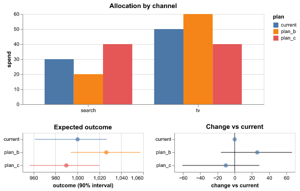
How to read it. plan_b moves 10 from search to TV. It is expected to bring 25 more revenue than 'current' (90% range 5 to 45), with a 99% probability to be better. plan_c is lower than 'current'.

Use it when

• You have a few budget plans and must pick one
• You want the probability that a new plan beats the current plan

Avoid it when

• You have only one plan (use Scenario vs baseline)
• The plans use spend far outside the history

What it needs

• A plans group: spend for each plan and channel, and draws of the outcome for each plan

What is on the chart

• Grouped bars of the spend in each channel for each plan
• A dot and a 90% range of the outcome of each plan
• A dot and a 90% range of the change from the reference plan
• A caption with the best plan and its probability to be better

For experts

Needs outcome draws. Outcome extra dims are summed. Ranges are HDIs at hdi_prob of the outcome and of (plan − reference) per draw; P(better) = share of draws with a positive difference. reference sets the reference plan; spend_var, outcome_var, plan and channel rename the inputs.

Effects between outcomes

mmm.cross_effects@1.0.0

Shows how a change in one outcome goes with a change in another outcome, for each pair that the model links. For example, more sales of a premium product can go with more sales of a basic product.

How to read it. A rise of one unit in premium sales goes with 0.26 more units of basic sales, and the range does not include zero. The link from basic to premium is not clear.

Use it when

• Your model has more than one outcome with links between them
• You want to know if products help each other (halo) or take sales from each other (cannibalisation)

Avoid it when

• The model has one outcome
• You want to prove cause and effect (the links are associations)

What it needs

• A cross_effects group: the effect of each source outcome on each target outcome, as draws, with the kind of each link

What is on the chart

• A dot and a 90% range for each link, coloured by kind
• A dashed line at zero
• A caption that names the links whose range does not include zero

For experts

Reads psi(sample, pair) with the coords source, target and kind on pair and the units in attrs['units']. Dots are medians, ranges HDIs at hdi_prob. The links act on the observed source outcome, so they mix the effect with correlated noise between the outcomes: read them as associations.

Contribution by component

mmm.decomposition@1.0.0

Splits sales (or another KPI) into the baseline and the part from each marketing channel. It shows each part over time and its total share.

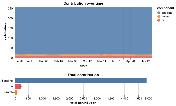
How to read it. The baseline gives 84% of revenue, TV 11% and search 5%. TV's range is narrow, so its share is clear. The range of search includes zero, so do not report its share as a fact.

Use it when

• You want to know how much each channel added in the period
• You report the effect of marketing to people who do not read models

Avoid it when

• You want the effect of future spend (use Response curves)
• The model has not converged

What it needs

• A contributions group split by channel, with draws, plus baseline variables

What is on the chart

• Stacked areas of the baseline and each channel over time
• Bars of the total contribution of each part with a 90% range
• A caption with the share of the top parts

For experts

Same computation as core.decomposition with component default 'channel'; variables without the channel dim (baseline, controls) become their own parts. Bars use the mean of each draw's total and an HDI at hdi_prob. Shares of a multiplicative (log-scale) model depend on the order of the parts, so read them as a guide.

Effect of spend over time

mmm.effectiveness@1.0.0

Shows the effect of one unit of spend in each period, for the channels whose effect can change over time. Use it to see if a channel becomes stronger or weaker.

How to read it. The effect of TV went from 2.0 to 1.45 for each unit of spend (−28%) in the year. It was highest in January. Search and social have a constant effect and do not show.

Use it when

• You fitted a model with time-varying channel effects
• You think that a channel lost (or gained) effect, for example after a creative change

Avoid it when

• No channel has a time-varying effect (the lines are then flat)
• You want the effect of more or less spend (use Response curves)

What it needs

• An effectiveness group: the KPI for each unit of spend in each period for each channel, as draws, and a flag for the time-varying channels

What is on the chart

• A line and a shaded 90% range for each time-varying channel over time
• A caption with the first and the last value and the period of the highest value

For experts

effectiveness(sample, channel, time) is Σ_cells steady-state KPI at the mean fit-window spend with the coefficient of period t, divided by that spend. Lines are medians, bands HDIs at hdi_prob. only_varying (default true) shows the channels with time_varying set (all channels when none is set); without the flag a channel varies when its median moves.

Lift tests and the model

mmm.lift_tests@1.0.0

Compares the result of each lift test with the value that the calibrated model gives for the same channel, period and market. It shows the tests that the model does not agree with.

How to read it. The model agrees with three of four tests. For lift_1 (search), the test measured 80 and the model gives 140. Look at the period and the market of that test, then at the prior of search.

Use it when

• You calibrated the model with lift tests and want to see if it agrees with them
• A test result looks strange and you want to compare it with the model

Avoid it when

• The model has no lift tests
• You want to know if the test itself is correct (the chart takes the test as given)

What it needs

• A lift_tests group: the result and the standard error of each test, and the model's value for each test as draws

What is on the chart

• Two rows for each test: the result of the test with its range (black) and the model's 90% range (blue)
• One panel for each kind of result (contribution or marginal ROAS)
• A caption that names the tests that the model does not agree with

For experts

Reads observed(test), observed_sd(test) and model(chain, draw, test) (or a sample dim) with the coords channel, estimand, start, end and geo on test. The model agrees with a test when its HDI at hdi_prob overlaps observed ± z × observed_sd (z = 1.96). Tests of different estimands get their own panel and scale.

Marginal cost

mmm.marginal_cost@1.0.0

Shows what the next unit of outcome costs in each channel at each level of spend. It can also show the return of the next unit of spend.

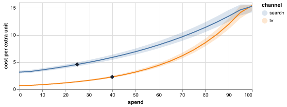
How to read it. At current spend, the next unit of revenue costs 0.8 in search and 2.5 in TV. The TV cost rises fast after 50. Move budget from TV to search until the two costs are close.

Use it when

• You want to move budget to where the next unit of outcome is cheapest
• You want to find the spend level where a channel stops paying back

Avoid it when

• You want total returns, not the return of the next unit (use Response curves)
• The response curves are very flat, so the cost is very large and uncertain

What it needs

• A response_curves group: draws of the response for each channel and spend level
• Optional: the current spend of each channel

What is on the chart

• A line for the median cost (or return) of each channel
• A shaded 90% band for each channel
• A diamond at the current spend of each channel
• A caption that names the cheapest channel at current spend

For experts

Per draw: slope = np.gradient(response, spend). metric='cost' plots 1/slope (NaN where the slope is ≤ 0); metric='roi' plots the slope. Values above the clip_quantile (default 0.98) of all finite values are capped, so the top of a band can be flat because of the cap. Median and HDI at hdi_prob. The value at current spend is interpolated on the median curve, not per draw.

Direct and mediated effects

mmm.mediation@1.0.0

Shows how much of the effect of each channel comes directly and how much comes through a mediator, such as site visits or brand awareness.

How to read it. 76% of the effect of TV goes through the mediators, most of it through awareness. Search works through visits. Social works directly: the ranges of its mediated paths include zero.

Use it when

• Your model has mediators between the channels and the KPI
• You want to know if a channel works through awareness or through visits

Avoid it when

• The model has no mediators
• You want to prove cause and effect (the paths depend on the structure of the model)

What it needs

• A mediation group: the direct effect and the effect through each mediator for each channel, as draws

What is on the chart

• A stacked bar for each channel: the direct part and one part for each mediator
• A line for the 90% range of the total effect
• A dot and a 90% range for the share of the effect through the mediators
• A caption with the largest share, the largest path and the paths whose range includes zero

For experts

Reads direct(sample, channel), indirect(sample, channel, mediator), total and share_mediated (computed from the others when missing). Bars stack the means (which add up); ranges are HDIs at hdi_prob. Effects are KPI totals over the fit window at actual spend. With a latent mediator only the product of the two path coefficients is identified; the chart shows it in KPI units.

Your beliefs and the priors

mmm.prior_beliefs@1.0.0

Compares the range that you gave for each channel with the values that the model allows before it sees your sales. Use it to check that the model understood your beliefs.

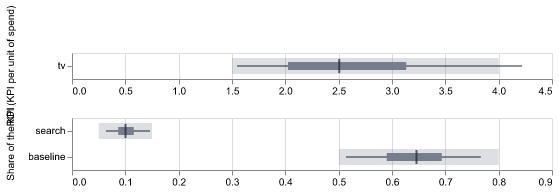
How to read it. You said TV's ROI is between 1.5 and 4.0 with 80% certainty. Only 60% of the model's values are in that range and the median is 2.5. The beliefs were translated too wide. Narrow the range or check the units of spend.

Use it when

• You entered beliefs about ROI or share for each channel
• You want to check the beliefs before you fit the model

Avoid it when

• You did not enter beliefs (the chart then has nothing to compare)
• You want the fitted results (use Contribution by component)

What it needs

• A prior_beliefs group: draws of ROI or share for each channel, and the ranges that you gave

What is on the chart

• A light band for the range that you gave
• A thin line for 90% of the model's starting values
• A dark bar for the middle 50% and a tick at the median
• One panel for each quantity (ROI, share)
• A caption with the share of values inside your range for each channel

For experts

Per channel, the stated quantity (roi or contribution_share, from stated_quantity) gives 5/25/50/75/95% quantiles of the prior draws; baseline_share with range attrs adds a baseline row. Coverage = share of prior draws inside [stated_low, stated_high], compared with stated_credibility. The height setting here is the height of one channel row (default 26).

Response curves

mmm.response_curves@1.0.0

Shows how much outcome each channel brings for each level of spend. A curve that becomes flat shows that more spend in that channel adds little.

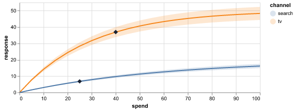
How to read it. The TV curve rises fast and becomes flat after 60. TV's diamond is at 40, on the flatter part. Search is still steep at 25. More money in search probably returns more than the same money in TV.

Use it when

• You want to know which channels are near saturation
• You plan the next budget and want to see the effect of more or less spend

Avoid it when

• You need the cost of the next unit of outcome (use Marginal cost)
• You want to read spend far above anything in the history

What it needs

• A response_curves group: draws of the response for each channel and spend level
• Optional: the current spend of each channel

What is on the chart

• A line for the median response of each channel
• A shaded 90% band for each channel
• A diamond at the current spend of each channel
• A caption that names the channel nearest to saturation

For experts

Median and HDI (hdi_prob, default 0.9) per channel and spend level; extra dims (such as geo) are summed. The spend axis is the grid coordinate or a spend_var over (channel, grid). The caption compares the slope of the median curve at current spend with its steepest slope (np.gradient). facet gives one panel per channel.

ROI and marginal ROI

mmm.roi@1.0.0

Shows the return of each channel for each unit of its current spend, and the return of the next unit of spend. A dashed line marks the point where a channel pays back its spend.

How to read it. Search has an ROI of 2.1 and social 0.55. The whole range of social is below 1.0, so social does not pay back its spend. TV has an ROI of 1.7, but its marginal ROI is 0.8: the next unit of TV spend returns less than it costs.

Use it when

• You want to know which channels pay back their spend
• You want to know where the next unit of budget brings the most
• You report the return of marketing to people who do not read models

Avoid it when

• The KPI and the spend are not in the same money units (the break-even line then has no meaning; set breakeven to None)
• You want the full curve of return against spend (use Response curves)

What it needs

• A response_curves group: the contribution of each channel for each spend level, with the current spend
• Optional: a marginal_cost group with the marginal ROI of each channel

What is on the chart

• A dot and a 90% range for the ROI of each channel
• A dot and a 90% range for the marginal ROI of each channel
• A dashed line at the break-even point (1.0 by default)
• A caption that names the best channel, the channels below the break-even point and the channels where the next unit returns less than it costs

For experts

Per draw: ROI = (f(current) − f(0)) / current, where f is the channel's response curve (extra dims such as geo summed) read by linear interpolation at current_spend (or at multiplier 1 when there is no current_spend). Marginal ROI comes from marginal_cost.marginal_roi_total when present, else from the slope (np.gradient) of each draw's curve at current spend. Dots are medians, ranges are HDIs at hdi_prob (0.9). breakeven (1.0, None for no line) draws the reference line and drives the caption. Channels with no spend have no ROI.

Share of spend and share of effect

mmm.spend_effect@1.0.0

Compares the share of the media budget that each channel gets with its share of the effect of all channels. A channel with a larger share of effect than of spend returns more than the average channel.

How to read it. Search gets 20% of the spend and brings 29% of the effect. Social gets 27% of the spend but brings only 10% of the effect. Social is a candidate for a smaller budget.

Use it when

• You want a quick view of which channels get too much or too little budget
• You present the results of a marketing mix model to people who do not read models

Avoid it when

• You want the return of the next unit of spend (use ROI and marginal ROI)
• Some channels have a negative effect (the shares then do not add up to 100%)

What it needs

• A response_curves group: the contribution of each channel for each spend level, with the current spend

What is on the chart

• A grey bar for the share of spend of each channel
• A blue bar and a 90% range for the share of effect of each channel
• A caption that names the channel with the best and the worst ratio of the two shares

For experts

Effects come from the response curves at current spend (as in mmm.roi). The share of effect is computed per draw (contribution of c / sum over channels) and shown as median and HDI at hdi_prob; the share of spend is current_spend / its sum. Channels without spend count as zero spend.

Contribution waterfall

mmm.waterfall@1.0.0

Shows how the baseline and each channel add up, step by step, to the total KPI of the period. The last bar is the total.

How to read it. The total is 5,760. The baseline parts give 81% and TV gives 11%, the most of the channels. The range of social includes zero, so do not report its part as a fact.

Use it when

• You want to explain the total sales of a period by its parts
• You present the effect of marketing in a report or a deck

Avoid it when

• You want to see the parts over time (use Contribution by component)
• The model is multiplicative, so the parts do not add up

What it needs

• A contributions group: the contribution of each channel and the baseline parts (baseline, trend, seasonality, controls), as draws

What is on the chart

• A bar for each baseline part, then for each channel from the largest to the smallest, then the total
• A line for the 90% range of each step
• A caption with the total, the baseline share and the largest channel

For experts

Each part is the sum over time and every non-channel dim per draw; the bar is the mean, the line the HDI at hdi_prob placed at the end of the step. Variables with a channel dim give one part per channel; other variables (and labels named baseline, trend, seasonality, intercept) are baseline parts. An outcome dim is reduced to outcome, else attrs['primary_outcome'], else its first level.

Network graph

net.graph@1.0.0

Shows a network as dots joined by lines, where thick lines are strong links. A second panel shows every pair of nodes as a grid of colours.

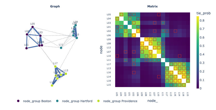
How to read it. The lawyers form three clusters that match their offices. Most known links are inside an office. Lawyer L11 links to all three clusters, so it is a bridge between the offices.

Use it when

• The model estimates links between pairs of things, such as people or genes
• You want to see groups of nodes that link to each other
• You want to compare the estimated links with the known links

Avoid it when

• There are more than 300 nodes (the drawing becomes too dense)
• The links change over time (pick one time with select)

What it needs

• A variable with two node dimensions, such as (node, node_): a probability, a weight or a partial correlation, as draws, a score summary or plain values
• Optional: node positions (node, latent_dim), a group for each node, and the known or observed links

What is on the chart

• A drawing of the nodes and the links above the threshold, with blue for positive and red for negative links
• Arrows when the links have a direction
• A grid of the link values for every pair, ordered so that groups are together
• Dotted lines and open squares for the known links

For experts

The edge value is the posterior mean (or the summary point). Undirected graphs use the mean of both directions; directed defaults to an asymmetric matrix and signed to any negative value. threshold defaults to 0.5 for values in [0, 1], else 10% of the largest |value|; hover shows P(|value| > threshold) over the draws. Positions are the posterior mean of positions (first two coordinates); else a spectral layout of the normalised Laplacian refined with seeded Fruchterman-Reingold steps. The matrix order is the Fiedler vector, within group levels.

Area map

sci.area_map@1.0.0

Shows a map of areas, such as districts, coloured by the model's estimate for each area. Other panels show the uncertainty and how likely it is that the value is above a limit.

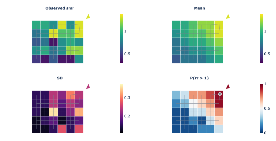
How to read it. The observed panel of lip cancer in Scotland shows extreme values in small districts. The mean panel is smoother. The probability panel is dark red in the north, and crosses mark the districts where the risk is above 1 with 95% probability.

Use it when

• The model gives one value for each area of a map, such as a disease risk
• You want to find the areas where the risk is clearly high
• You want to compare the smoothed estimate with the raw observed values

Avoid it when

• The output is a value on a regular grid (use Field map)
• You need a base map with roads and place names (the chart draws only the outlines)

What it needs

• Draws of a per-area output in the posterior, predictions or posterior_predictive group (a summary with mean and sd also works)
• The outlines of the areas as ring_x(area, vertex) and ring_y(area, vertex)
• Optional: observed values for each area and a neighbour matrix adjacency(area, area_)

What is on the chart

• One map panel each for the observed values, the mean and the SD
• A panel with the probability that the value is above the threshold
• Crosses on the areas where that probability is above 95%
• Optional grey lines between neighbouring areas

For experts

Statistics per area over up to max_draws (2000) draws: mean, median, sd (ddof 1) and P(value > threshold) (stats; default observed, mean, sd and exceedance). threshold defaults to 1 for a non-negative output (a relative risk) and to 0 otherwise. Fills use classes (9) equal steps of the colour scale over the 0.5 to 99.5% range; the colour bar and the hover show the exact value. log_scale colours log10 of the value panels. Areas match the outlines by label when both have labels, else by position. Polygons are drawn as filled scatter shapes on equal-aspect axes, not a geographic projection.

Ensemble of draws

sci.ensemble@1.0.0

Shows many possible paths from the model as thin lines, with a shaded range and the actual values. Use it to see what single outcomes can look like, not only the average.

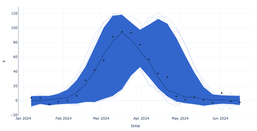
How to read it. Most thin lines rise to a peak in week 10, but some peak in week 14. The band is wide around the peak. The dots are inside the band, so the model allows the actual peak, but it is not sure of the timing.

Use it when

• You want to see the shapes that the model allows, such as peaks and dips
• You want to explain uncertainty to people with single example paths

Avoid it when

• You want a clean summary for a report (use Fit and forecast)
• The output has more than one dimension that you cannot fix to one level

What it needs

• Draws of an output in the predictions, posterior_predictive or posterior group
• Optional: the actual values (observed_data group)

What is on the chart

• Thin lines for 40 single draws
• A shaded 90% band
• A thick line for the median
• Dots for the actual values
• A caption with the share of actual values inside the band

For experts

n_draws (40) lines chosen without replacement with seed; bands are equal-tailed quantiles at levels (default [0.9]) over up to max_draws (2000) draws. point is median, mean or none. along defaults to the time-like dim, else the grid's x. Other dims must have one level or be fixed with select. The median line is not itself a possible path.

Field map

sci.field_map@1.0.0

Shows a map of a value that the model estimates on a grid, such as a density over an area. One panel shows the average and another panel shows where the model is not sure.

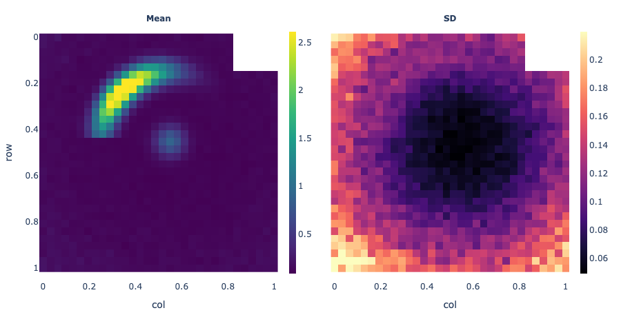
How to read it. The mean panel of a lensed galaxy shows a bright arc at the top left. The SD panel is dark there and bright at the edges of the image. The arc is clear, and the edges are not fixed by the data.

Use it when

• The model gives a value for each cell of a 2D grid (an image or a map)
• You want to see where the data fixes the value and where it does not

Avoid it when

• The output has no grid (use Profiles with bands or Ensemble of draws)
• The output is a direction and a length (use Vector field)

What it needs

• Draws of a gridded output in the posterior, predictions or posterior_predictive group
• Two grid dimensions, from the output's grid declaration or the settings

What is on the chart

• A heatmap of the mean in each cell
• A heatmap of the SD (the uncertainty) in each cell
• Optional panels: median, mean ÷ SD, 5% and 95% values, and a few single draws
• A slider when the output has a frame dimension, such as time

For experts

Statistics per cell over up to max_draws (400) evenly thinned draws: mean, median, sd (ddof 1), z = mean/sd, q05, q95 and n_draws single draws (stats, default mean and sd). log draws log10 first. Rasters are block-averaged to stay under max_cells per panel. colormap, origin and log default to the grid declaration. frame adds a slider (up to max_frames); select fixes other dims.

Image residuals

sci.image_residuals@1.0.0

Shows the observed image, the image that the model expects and the difference between them. A pattern in the difference shows something that the model misses.

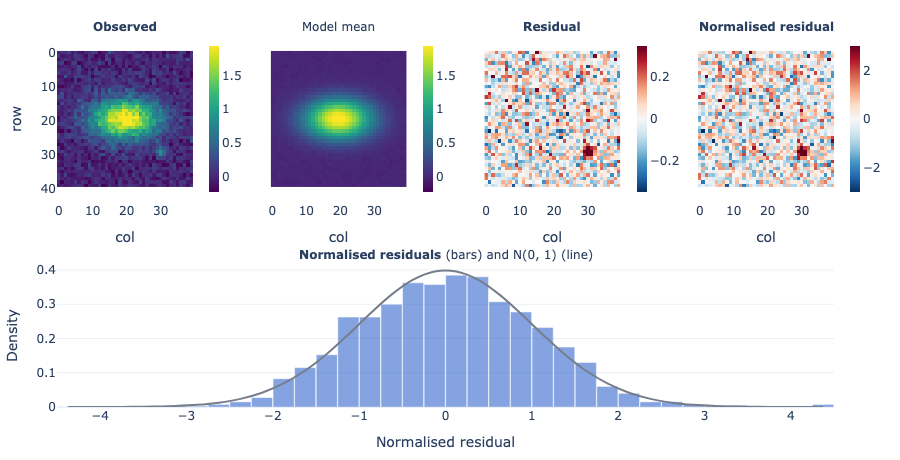
How to read it. The residual of a galaxy image is grey noise except for a red spot at the bottom right. The model has the main galaxy but not a small companion next to it. The normalised residuals have an sd of 1.04, so the noise level is right.

Use it when

• The model makes an image or a map that you can compare with a measured one
• You want to find the parts of the image that the model does not explain
• You want to check that the noise in the model has the right size

Avoid it when

• There is no observed image (use Field map)
• You want to see single images from the model (use Predictive image grid)

What it needs

• Draws of a gridded output in the posterior_predictive, predictions or posterior group
• The observed image with the same grid (observed_data group)
• Optional: the noise of the data (a sigma variable or a number)

What is on the chart

• Heatmaps of the observed image and the model mean on one colour scale
• A heatmap of the residual (observed minus mean) on a red-blue scale
• A heatmap of the residual divided by the uncertainty and the noise
• A histogram of these normalised residuals with the standard normal curve
• A slider when the output has a frame dimension

For experts

Mean and sd (ddof 1) per cell over up to max_draws draws; residual = obs - mean; normalised = residual / sqrt(sd² + σ²). σ² comes from sigma (a variable: posterior draws are averaged as E[σ²]; or a number), read as sigma_kind sd, variance or inverse_variance. Without sigma, a variable named sigma is used, but only for noise-free images: draws from posterior_predictive already hold the noise. The histogram uses all cells at full resolution, bins of 0.25 on [-4.5, 4.5] (the tails go to the end bins). log colours the observed, mean and residual panels as log10 (the residual is a log10 ratio); the normalised residual stays in data units, as σ is.

Phylogeny with tip estimates

sci.phylogeny@1.0.0

Shows a family tree of species next to the model's estimate for each species. Close relatives sit side by side, so you can see if related species have similar values.

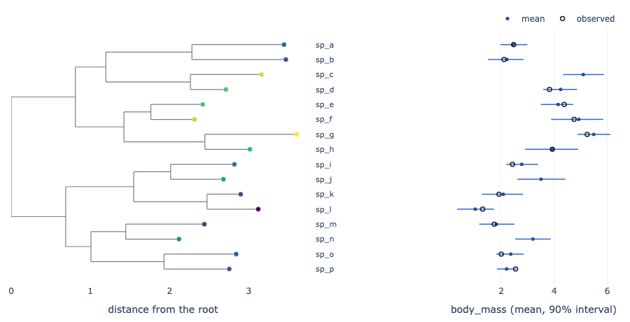
How to read it. The tree of 16 primates puts the large apes together at the top. Their dots in the strip are all on the right. Three species have no observed body mass, and their intervals are a little wider than those of their relatives.

Use it when

• The model gives one value for each species (or other tip) of a tree
• You want to see how the estimate follows the tree
• Some species have no observed value and you want to see their estimate

Avoid it when

• The groups are not related by a tree (use Posterior forest)
• The tree has thousands of tips and you need to see every one of them

What it needs

• Draws of a per-tip output in the predictions, posterior_predictive or posterior group
• The tree as parent(node) and branch_length(node), with optional is_tip(node) and tip_label(node)
• Optional: the observed trait for each tip (observed_data)

What is on the chart

• The tree with the branch lengths along the x axis
• A dot at each tip coloured by the estimate
• A strip with the estimate and its 90% interval for each tip
• Open circles for the observed values

For experts

The layout is rectangular: x is the sum of branch lengths from the root, y the order of the tips in a depth-first walk; a parent sits midway between its outer children. parent holds integer positions (or node labels); -1, NaN or the node itself marks a root, and several roots join at a common origin. The strip shows the mean or median (point) and the equal-tailed interval (0.9). max_tips (400) keeps evenly spaced tips and their ancestors.

Point pattern

sci.point_pattern@1.0.0

Shows points, such as events or light sources, at their positions on a map or an image. A ring around each point shows where its true position can be.

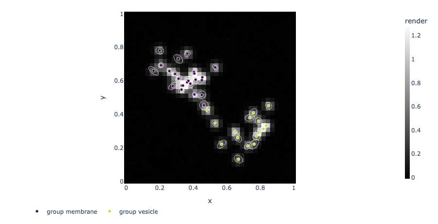
How to read it. Spots in the membrane have small rings, so their positions are clear. Two dim spots have large, tilted rings: they could be one spot or two near spots.

Use it when

• The model finds the positions of points, such as molecules in a microscope image
• You want to see which positions are certain and which are not
• You want to compare the points with an image or a map of the intensity

Avoid it when

• The output is a value on a grid without points (use Field map)
• There are more than 20 000 points (the plot shows a thinned set)

What it needs

• Variables x and y with one value for each point, as draws, a score summary or plain values
• Optional: sd_x and sd_y (or radius) for each point, a group for each point, and a gridded output for the background

What is on the chart

• A dot for each point at its mean position, coloured by group
• A ring (an error ellipse) for each point that holds its true position with 90% probability
• A background image or intensity map
• Open circles for the actual points, when the data has them

For experts

Positions are the posterior mean of x and y (or the summary's point statistic). Ellipses use the 2 x 2 sample covariance of the draws (else sd_x, sd_y or the summary sd, uncorrelated) scaled by sqrt(-2 ln(1 - level)), the chi-square radius for 2 dims; a radius variable is drawn as a circle as given. field (auto: a grid output) is drawn as the field_stat per cell, block-averaged to max_cells. group draws with more than 12 levels use a colour scale.

Power spectrum

sci.power_spectrum@1.0.0

Shows how much signal there is at each scale or frequency, as the model sees it, with shaded ranges and the measured points.

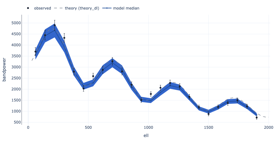
How to read it. The model's spectrum of a sky patch follows the dashed theory curve at large scales, but it is lower than the curve above multipole 1500. 75% of the observed points are in the 90% band, so the patch has a little less power at small scales.

Use it when

• The model gives a spectrum in bins, such as the power of a sky map or a signal
• You want to compare the spectrum with a theory curve and with the data

Avoid it when

• The output is not binned along one dimension (use Profiles with bands)
• You want single possible spectra (use Ensemble of draws)

What it needs

• Draws of a binned output, with a coordinate such as multipole or frequency
• Optional: observed values and their sd (observed_data group)
• Optional: a theory curve in any group

What is on the chart

• A line for the median in each bin
• Shaded 50% and 90% bands
• A dashed theory curve
• Dots for the observed values with error bars
• A caption with the share of observed values inside the 90% band

For experts

Equal-tailed bands at levels (default 0.5, 0.9) and the median or mean over up to max_draws draws. x is x_coord (default: the first numeric coord on the bin dim, such as ell; else the bin index). theory is any variable along one dim (draws give the median). Error bars are error_var, default <observed>_sd. log_x and log_y set log axes. The recipe draws the spectrum as given; scale it (for example to D_ell = ell(ell+1)C_ell/2π) in the model.

Predictive image grid

sci.ppc_image_grid@1.0.0

Shows the observed image next to a few images that the model makes. If the model fits, it is difficult to tell which image is the real one.

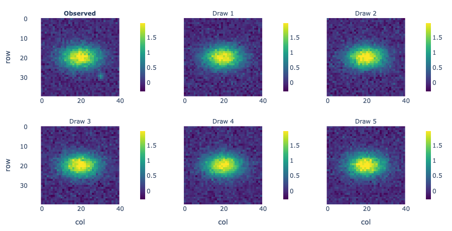
How to read it. In a shuffled grid of six patterns, five look the same and panel D has thinner stripes. The caption says that panel D is the real image, so the model makes stripes that are too wide.

Use it when

• You want a quick visual check that the model can make images like the data
• You want to test yourself or others with a shuffled grid

Avoid it when

• You want to locate the errors cell by cell (use Image residuals)
• There is no observed image (use Field map with draws)

What it needs

• Draws of a gridded output, best from the posterior_predictive group
• The observed image with the same grid (observed_data group)

What is on the chart

• One heatmap of the observed image and one for each draw, on one colour scale
• With shuffle, the panels are in a random order and the caption names the real one
• A slider when the output has a frame dimension

For experts

n_draws (5) draws chosen without replacement with seed; shuffle permutes the observed panel among them with the same seed. All panels share one value range (0.5 to 99.5 percentile). This is the visual 'line-up' test of Buja et al. (2009) and Gelman's graphical posterior predictive checks.

Profiles with bands

sci.profile_bands@1.0.0

Shows the model's estimate along one dimension, such as distance, with shaded ranges. It draws one curve for each level of a second dimension, such as time.

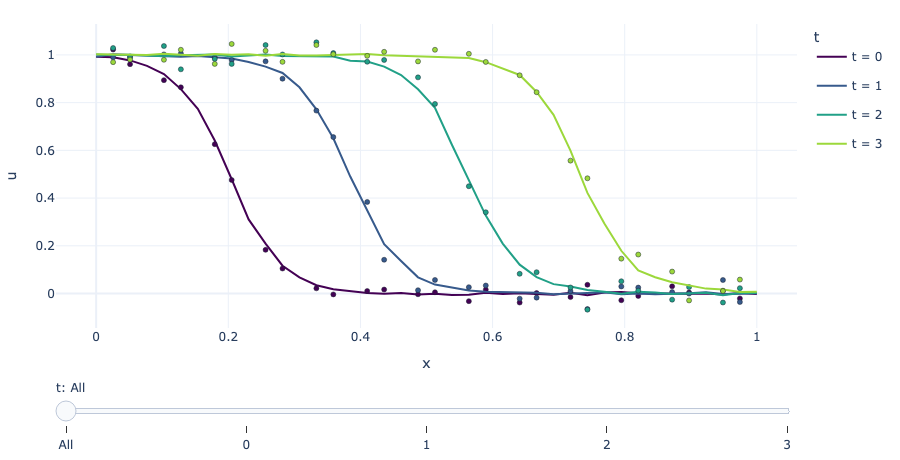
How to read it. Each line is the population along the river on one day. The front moves right and the bands become wider on later days. 88% of the dots are in the 90% band, so the model follows the spread of the population.

Use it when

• The model gives a curve, such as a profile over space at several times
• You want to compare the curves with the actual values

Avoid it when

• The output is a 2D map that you want to see as a picture (use Field map)
• You want to see single possible paths (use Ensemble of draws)

What it needs

• Draws of an output in the predictions, posterior_predictive or posterior group
• Optional: the actual values (observed_data group)

What is on the chart

• A line for the median of each curve
• Shaded 50% and 90% bands for each curve
• Dots for the actual values
• A slider that shows one curve with its bands at a time
• A caption with the share of actual values inside the 90% band

For experts

Median or mean and equal-tailed quantile bands at levels (default 0.5, 0.9; at most 3) over up to max_draws draws. along defaults to the grid's x; by to the grid's frame or y. max_curves (12) picks evenly spaced levels of by. The slider's 'All' step shows the lines without bands. Coverage uses the widest band. log sets a log y axis.

Rose of angles

sci.rose@1.0.0

Shows directions or times of day on a circle. Bars show how often each direction occurs, with the range that the model expects for each sector.

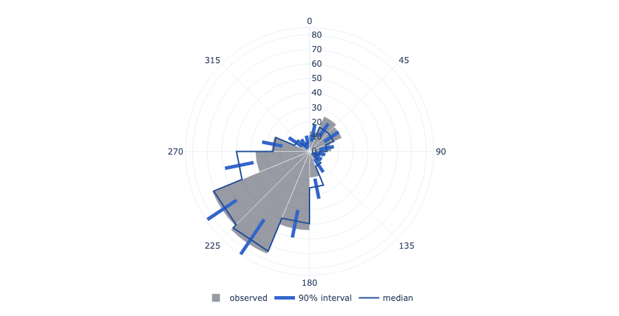
How to read it. The rose of wind directions has a long bar to the south-west. The model's range covers it, but the bars to the north-east end above the range: the model gives too few winds from the north-east.

Use it when

• The data are angles, such as wind directions, hours of the day or days of the year
• You want to check that the model gets the main directions right
• The model gives a density around the circle and you want to see its shape

Avoid it when

• The values are not on a circle (use Posterior predictive check)
• You need the exact numbers for each direction (use a table)

What it needs

• Observed angles (observed_data) and draws of simulated angles (posterior_predictive), or a density over an angle dimension with draws
• The units of the angles: radians, degrees, hours or days

What is on the chart

• Bars for the observed count (or share) in each sector
• A thick line in each sector for the 90% range of simulated data, and the median
• Or a median curve with dotted 90% limits
• A slider when the data have a frame dimension, such as season

For experts

Histogram mode: the observed angles and each of up to max_draws (1000) predictive draws are counted in bins (24) equal sectors; the lines are equal-tailed interval (0.9) quantiles of the counts per sector. scale share divides by the number of angles (the default with a frame). Density mode (an angle_dim such as angle, hour or direction): quantiles per angle; observed angles are scaled to a density per unit. clockwise defaults to true (zero at the top) except for radians.

Colour swatches

sci.swatches@1.0.0

Shows squares in the colours that the model gives to each item, next to the measured colours. Squares that change from draw to draw show where the model is not sure.

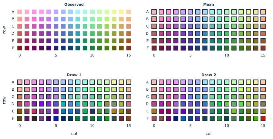
How to read it. On the chip map, the mean squares match the measured squares in the light rows. In the dark rows the draws change from green to brown, so the model is not sure of the dark colours.

Use it when

• The model gives a colour for each item, such as a paint, a chip or a pixel
• You want to compare model colours with measured colours by eye
• The items have places on a chart, such as the colour-naming chip chart

Avoid it when

• The output is not a colour in sRGB from 0 to 1 (convert it first)
• You need exact colour differences (read the numbers instead)

What it needs

• Draws of an output with an item dimension and an rgb dimension of length 3
• Optional: measured colours with the same dimensions (observed_data group)
• Optional: row and col coordinates on the item dimension to draw a map
• Optional: a probability for each item, shown as border width or opacity

What is on the chart

• Squares of the measured colours
• Squares of the mean colour and of a few single draws
• A list of items, or a map when the items have row and col coordinates
• A caption with the mean distance between model and measured colours

For experts

channel (rgb) is the length-3 dim, reordered to r, g, b by its labels. Colours are written as hex strings in the dataset. arrange auto draws a map when row and col coords exist on the item dim (text coords become ordered ticks). prob (draws are averaged) sets border width (0 to 2.5 px) or opacity (prob_as) on the model panels. A list shows at most max_items evenly spaced items. The distance in the caption is the Euclidean sRGB distance on a 0 to 255 scale, not CIEDE2000.

Vector field

sci.vector_field@1.0.0

Shows a field of arrows, such as forces or flows, on a grid. Colours show the length of the arrow in each cell and a second panel shows where the length is not certain.

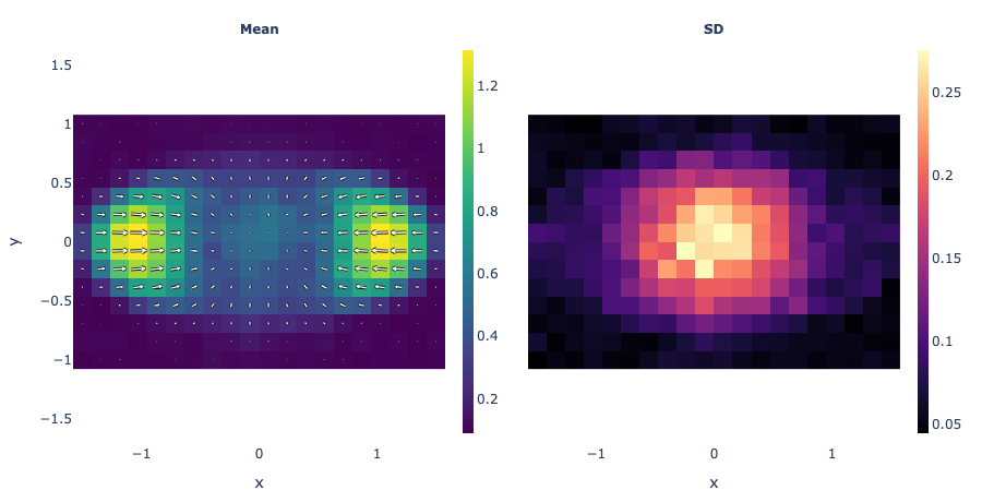
How to read it. The arrows of a cell's traction force point inwards at the edges of the cell. The colours are bright at the two ends, where the forces are largest. The SD panel is high in the centre, so the forces there are not certain.

Use it when

• The model gives a direction and a length for each cell of a 2D grid
• You want to see the pattern of a flow or a force

Avoid it when

• The output has one value for each cell (use Field map)
• The directions change a lot between draws (the mean arrows then look too short)

What it needs

• Draws of a gridded output with a component dimension of length 2 (the x and y parts)

What is on the chart

• A heatmap of the mean length with arrows of the mean direction
• A heatmap of the SD of the length
• Optional panels: the 5% and 95% values of the length
• A slider when the output has a frame dimension

For experts

Length = hypot(u, v) per draw; panels are its mean, sd, q05 or q95 (stats). Arrows are the mean (u, v), block-averaged to about arrows (20) along the longer side and scaled so the longest is 0.9 of the arrow spacing. The mean length is at least the length of the mean vector; they differ when directions vary. component names the length-2 dim (default: the grid's, else the only one).