E18 Scottish lip cancer disease map (ICAR/BYM2)

This tutorial does the main analysis of the pymc-challenges notebook E18_areal_models_icar_bym2.py in the web app. You use the model sci.areal_bym2@1. You do not write PyMC code.

You need:

• The platform (start it with make dev) and a project that you can upload datasets to. This tutorial uses the project epidemiology. If your project has a different name, change the project part of each dataset:// and model:// reference.
• A local copy of pymc-challenges. The export command reads the file data/scotland_lip.geojson.
• About 15 minutes. One fit takes less than one minute of sandbox time.

1. The question

Between 1975 and 1980, 536 men in Scotland got lip cancer. For each of the 56 districts, you know the observed count and an expected count. The expected count is the count of the district if each age group had the national rate. The ratio of the two is the standardised morbidity ratio (SMR). The SMR is a raw estimate of the relative risk of the district.

The notebook asks two questions:

1. Where is the risk really high, when you include the noise of small counts?
2. Does outdoor work explain the risk? AFF is the percentage of the workers in agriculture, fishing and forestry. Lip cancer has a relation to sunlight.

Small districts have few cases, so their SMRs have much noise. The notebook lets each district share its risk with its neighbours on the map. It puts graph priors on the district effects: the intrinsic CAR (ICAR), the proper CAR and BYM2. BYM2 is a scaled ICAR plus independent effects. Its parameter rho is the share of the variation that follows the map.

The decision at the end of the notebook is this:

• Do not publish the raw SMR map. Publish the BYM2 smoothed relative risk and the probability that the relative risk is more than 1. In 19 districts this probability is more than 0.95. These are the districts where the risk is "high and certain".
• Use BYM2 as the default model. The graph models predict equally well, and all three predict better than independent districts. BYM2 has a rho that you can read, and its priors mean the same thing on each map.
• Report the AFF effect as an association. Its 90% interval excludes 0 in each model. But its size changes from a relative risk of 1.96 for each 10 points (independent districts) to 1.50 (BYM2). The size depends on what you assume about risk factors that you did not measure. This is spatial confounding.

What you will get, and the notebook section that each item replaces:

In the web app	Notebook
The graph of the districts, with the island links (Plots, net.graph)	Section 2 (the queen graph) and section 3 (the island links)
The posterior of b0, b1, sigma and rho (Parameters)	Section 4, the BYM2 row of the diagnostics table, and section 6
The smoothed relative risk rr and p_exceed, the probability that rr is more than 1 (Plots, sci.area_map)	Section 7, the three maps
elpd_loo and the Pareto k warning (Diagnostics)	Section 8, the LOO table
The error on 7 districts that the fit did not see (Diagnostics)	Section 8, a smaller version of the 8-fold cross-validation
The ladder of kind values, compared by elpd_loo (the recipe sci_spatial_ladder)	Section 4 (the five models) and section 9 (b1 in each model)
New maps of risk and counts (Score, Simulate)	Section 3, the prior predictive draws "by hand"

Some parts of the notebook are not in the port, for example the unscaled BYM and the Moran's I checks of the residual effects. See Differences from the notebook.

2. Get the data

The export command reads the GeoJSON file of pymc-challenges and writes a NetCDF file that the platform can read. Run it from the root of the modeling-api repository:

uv run python -m mapi_plugin_science.export e18 \
    --challenges <path to pymc-challenges>/data \
    --out scotland_lip.nc --spec scotland_lip.yaml

The command writes:

wrote scotland_lip.nc (variables cases, expected, aff, adjacency, ring_x, ring_y on district=56, district_=56, vertex=51)
upload it as dataset epidemiology/scotland_lip_cancer and fit sci.areal_bym2
wrote the suggested spec to scotland_lip.yaml

The file holds one dataset:

Name	Dims	Type	Meaning
district	56	categorical, fixed	The district names, as in the GeoJSON file (Orkney has the name Okney)
district_	56	categorical, fixed	The same districts again: the second axis of adjacency
vertex	51	integer, fixed	The points of the outline of each district
cases	district	float64, target	The observed cases, 1975 to 1980 (CANCER)
expected	district	float64, exposure	The expected cases (CEXP), from 1.07 to 88.66
aff	district	float64, covariate	The percentage of workers in agriculture, fishing and forestry (AFF)
adjacency	district, district_	int64, constant	1 when two districts touch (queen contiguity), else 0
ring_x, ring_y	district, vertex	float64, constant	The outline of each district in British National Grid metres. NaN fills the unused points

The export makes the graph as the notebook does. Two districts are neighbours when their outlines share at least one point. The graph has 117 edges. Orkney, Shetland and the Western Isles have no neighbours. The model links them when it fits (step 6.1).

The attribute mapi_schema gives each variable its role, so you do not map columns.

Simulated data

--synthetic writes a map of 43 square districts (one of them is an island) with counts from the model itself. The true values are b0 = 0.1, b1 = 0.4, sigma = 0.5 and rho = 0.8. You do not need pymc-challenges for it.

uv run python -m mapi_plugin_science.export e18 --synthetic --out disease_map_synthetic.nc

3. Upload the dataset

1. Open Datasets in the sidebar.
2. Click New dataset.
3. Type scotland_lip_cancer in Name. Type a description, for example "Male lip cancer in 56 districts of Scotland, 1975 to 1980, with district outlines".
4. Click Create dataset. The upload panel opens.
5. Click Choose files and select scotland_lip.nc.
6. Click Preview structure. The panel shows Structure of the file. Make sure that it shows cases, expected and aff on district, and adjacency on district and district_.
7. Optional: type a message in Version message (optional).
8. Click Upload and ingest.

The ingest run reads the file in the sandbox. When it is done, the version page shows the tabs Schema, Coordinates, Missingness, Preview and About. On Schema, cases has the role target, expected has the role exposure and aff has the role covariate. Missingness shows missing values only in ring_x and ring_y. These are the unused points of the shorter outlines.

The file is one plain dataset. You do not need the tree fields ("Put this file in a node of a tree (optional)") or the HDF5 path.

3.1 Explore the data

Look at the data before you build the spec.

1. On the version page, click Explore this version. The Data Explorer opens. The sections under Pictures of the data come first.

2. Click Map.

3. The map shows the 56 districts. Select cases, expected, aff or the ratio cases / expected (the standardised morbidity ratio) to set the colours. The lines join the neighbour districts.

4. The list of areas with no neighbour shows the labels of the data: Okney (Orkney), Shetland and WesternIsles (the Western Isles). The model links them when it fits (step 6.1).
5. The table of Moran's I tells if neighbour districts have similar values. A positive value with a small p-value is a reason for a spatial model.
6. ring_x, ring_y and adjacency are geometry. They are not in Distributions, Unusual values or Data quality.
7. The time sections are in Not for this data. The data has no time dim.

Refer to Scientific data.

4. Build the spec

1. Open Build and click New spec. The editor opens with the geo MMM template.
2. Set the Editor view to YAML.
3. Open the Insert panel on the right.
4. Open the Datasets section and select scotland_lip_cancer. The toast "Dataset set" shows.
5. Type areal in the search field. Under Models, select Disease risk on a map of areas (sci.areal_bym2@^1). The toast "Model set" shows.
6. Select all the text in the editor and paste the full spec below. The template has other blocks (a pipeline, a split and the MMM plots), so the spec must replace all of it.
7. Click Validate. The status shows valid.
8. Click Save spec. The spec gets its name scotland-lip-cancer-bym2 from metadata.name.

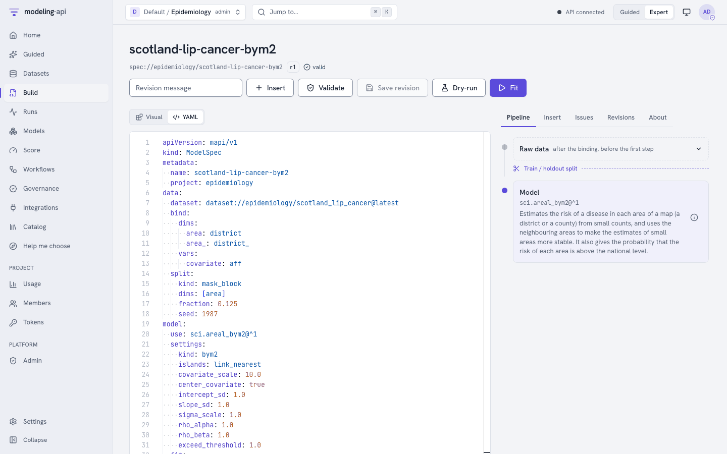
This is the full spec:

apiVersion: mapi/v1
kind: ModelSpec
metadata:
  name: scotland-lip-cancer-bym2
  project: epidemiology
data:
  dataset: dataset://epidemiology/scotland_lip_cancer@latest
  bind:
    dims:
      area: district
      area_: district_
    vars:
      covariate: aff
  split:
    kind: mask_block
    dims: [area]
    fraction: 0.125
    seed: 1987
model:
  use: sci.areal_bym2@^1
  settings:
    kind: bym2
    islands: link_nearest
    covariate_scale: 10.0
    center_covariate: true
    intercept_sd: 1.0
    slope_sd: 1.0
    sigma_scale: 1.0
    rho_alpha: 1.0
    rho_beta: 1.0
    exceed_threshold: 1.0
  fit:
    mode: evaluate_then_refit
    seed: 1987
    tune: 1000
    draws: 1000
    chains: 4
    target_accept: 0.9
    engine: nutpie
evaluate:
  metrics: [rmse, mae, coverage_90, elpd_loo]
outputs:
  plots:
    - core.convergence
    - core.posterior_forest
    - sci.area_map
    - net.graph

The settings are the defaults of the model. They are also the choices of the notebook. The --spec file of the export has the short form of the same spec. This table tells what each setting means for the question:

Setting	Value	Meaning for this question
kind	bym2	The prior of the district effects. bym2 is the model that the notebook recommends. Use poisson, iid, icar or car to fit the other models of the notebook (step 6.5)
islands	link_nearest	Orkney, Shetland and the Western Isles have no neighbours. The model links each one to the district with the closest outline, as the notebook does. Without a link, the BYM2 scaling factor is not defined
covariate_scale	10	b1 is the effect of 10 percentage points of AFF on the log relative risk, as in the notebook
center_covariate	true	The model subtracts the mean AFF (8.66%). Thus b0 is the log relative risk of a district with a mean AFF
intercept_sd, slope_sd	1, 1	The priors b0 ~ Normal(0, 1) and b1 ~ Normal(0, 1) of the notebook
sigma_scale	1	The prior sigma ~ HalfNormal(1) of the total sd of the district effects
rho_alpha, rho_beta	1, 1	The prior rho ~ Beta(1, 1): all shares are equally probable before the data
exceed_threshold	1	p_exceed is the probability that rr is more than 1, that is, more than the national rate

• bind gives the dataset names to the names of the model. The model calls the districts area and the covariate covariate. The outputs come back with your names.
• split holds out 12.5% of the districts (7 districts). The model keeps these districts in the graph, but it does not use their counts. It predicts them from their neighbours. This is the question "what is the risk in a district without data?" of notebook section 8.
• fit.mode: evaluate_then_refit first fits without the held-out districts and calculates the metrics on them. Then it fits again on all 56 districts. The parameters and the maps come from the second fit.
• engine: nutpie is the sampler of the notebook. engine: pymc gives the same result, but it is slower.
• The model always keeps the log-likelihood of each district, so you do not need a keep block for elpd_loo.

The plots

The model declares core.convergence, core.posterior_forest, sci.area_map, net.graph and core.ridge. The fit makes only the plots in outputs.plots. core.ridge needs the setting dim, and a spec cannot give settings to a plot. Without dim, the fit skips the plot with the issue SCHEMA_INVALID. Thus the spec does not name core.ridge.

5. Fit and watch the run

1. Click Fit. The app opens the run page.
2. The badge shows Live while the run sends events.
3. The Progress card shows the progress of the sampler. The run fits two times: first without the 7 held-out districts, then on all 56 districts. The Events card shows the stages of the run and, at the end, the diagnostics. The Logs card stays empty when the model writes no output.
4. When the run is done, the Result card shows Inspect model://epidemiology/scotland-lip-cancer-bym2@v1. Click it.

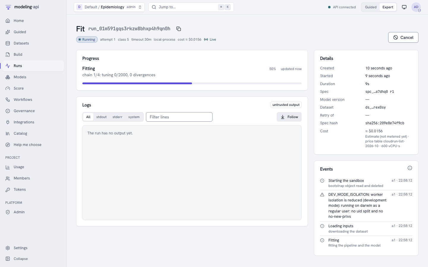
The two fits took 21 s in our test. Each fit samples b0, b1, sigma, rho and two effects for each district (phi for the ICAR part and theta for the independent part).

You can also find the run under Runs. Filter it with the kind fit.

6. Read the result

On the model version page, the tabs are Overview, Diagnostics, Plots, Data tree, Preprocessing and Provenance. Click Explore to open the Model Explorer.

The outputs of this model are on the districts, not on a grid. Thus the Fields section is under "Does not apply". Fit vs actual and Residuals also show there, because they need a time dimension. The maps are in the Plots tab of the model version page.

Open Overview to see the scorecard. The check "Few missing values" passes. It counts only the variables that contain observations. Thus it does not count the padding of the outlines ring_x and ring_y (and adjacency), because they have the role constant. The expert message names these variables.

6.1 The graph that the model used

The model links the three islands before it fits. The bundle of the version keeps the result in learned:

Value	Result	Notebook
n_components_input	4 (the mainland and three islands)	4 connected components
islands_input	Okney, Shetland, WesternIsles	the same
links	Okney to Caithness (28 km), Shetland to Okney (192 km), WesternIsles to Ross-Cromarty (41 km)	the same links and distances
n_edges	120	120
scaling_factor	0.632	0.632

The link from Shetland is 192 km long, because the GeoJSON file draws only the north part of Shetland. The rule still selects Orkney, as in the notebook.

On the model version page, open Plots and select the plot with the title "Network of adjacency" (net.graph). It draws the 120 links at the centres of the districts, next to the full adjacency matrix. Look for the three long links to the islands in the north and the north-west.

6.2 Can you trust the fit?

Open Diagnostics in the Model Explorer (group "Can you trust it?").

• The largest R-hat is 1.006 (phi), the smallest bulk ESS is 588 (rho) and there are 0 divergences. The sampler has no problems.
• TREE_DEPTH shows that 1 of 4000 draws hit the largest tree depth. This is information only. The results are correct.
• PARETO_K_HIGH is a warning: 17 of 56 districts have a Pareto k above 0.7. This is expected. Each district has its own effect, so when PSIS-LOO removes the count of a district, the posterior changes too much. The notebook found 24 such districts. Do not quote elpd_loo as a precise value.

The diagnostics also show the metrics of the 7 held-out districts (Wigtown, Badenoch, Inverness, Kyle-Carrick, Dumbarton, Edinburgh and East Kilbride). The model predicted their counts from their neighbours only:

Metric	Value	Meaning
rmse	7.64 cases	The error of the predicted counts. Edinburgh has 50.7 expected cases, so a large error in cases is possible
mae	4.81 cases	The mean absolute error
coverage_90	1.00	All 7 observed counts are in their 90% intervals
elpd_loo	−153.0	PSIS-LOO of the fit on all 56 districts (notebook: −152.7)

6.3 What the model learned

Open Parameters (group "What it learned"). The table shows the posterior mean and the 90% highest-density interval:

Parameter	Mean	90% interval	Meaning
b0	0.102	0.003 to 0.206	The log relative risk of a district with a mean AFF. Scotland has 11% more cases than the expected counts give
b1	0.406	0.201 to 0.625	The effect of 10 points of AFF on the log risk. exp(0.41) = 1.50 for each 10 points
sigma	0.518	0.382 to 0.656	The total sd of the district effects on the log scale
rho	0.802	0.569 to 1.000	The share of the district variation that follows the map

The table also has 56 rows each for rr, effect, phi and theta.

The answer to "how much of the risk follows the map?" (notebook section 6) is rho. Its median is 0.84 and its 90% interval is wide. Most of the variation after AFF is spatial. A district's risk is better predicted by its neighbours than by an independent quirk of the district. Thus there are possibly more risk factors that change smoothly over Scotland, and that AFF does not include.

6.4 The maps

On the model version page, open Plots:

Plot	What to look for
Sampler convergence (core.convergence)	The text says "All 228 parameters look converged."
Posterior forest (core.posterior_forest)	The intervals of step 6.3 and of each district. b1 is clearly above 0
Area map (sci.area_map)	The title is "Area map of rr". This is the map of notebook section 7. See below
Network (net.graph)	The title is "Network of adjacency". The graph of step 6.1

The area map has four panels for the relative risk rr:

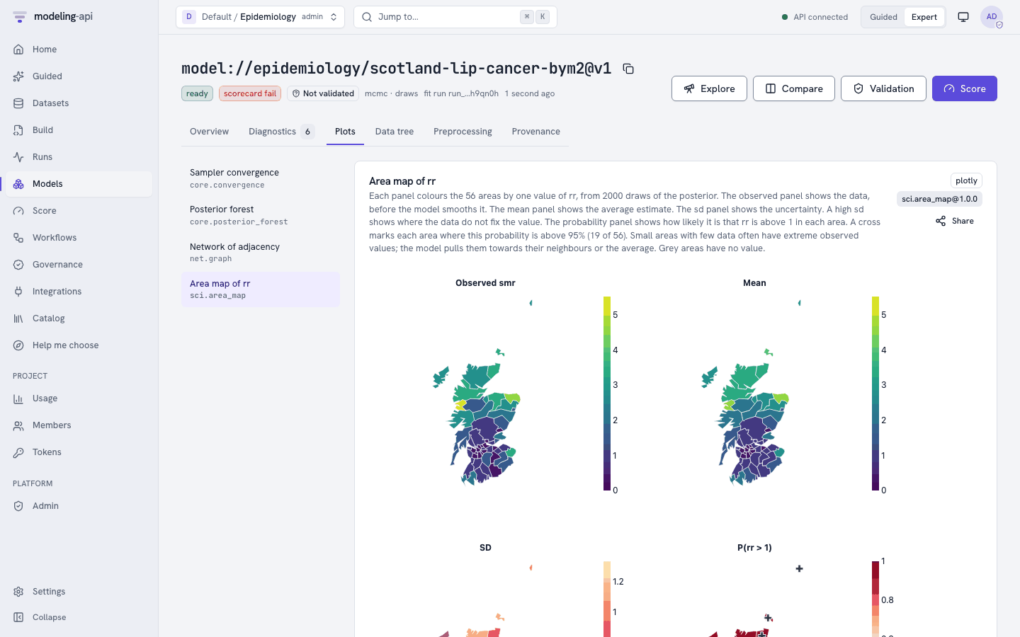
• Observed smr: the raw SMR (observed ÷ expected). The extreme colours are on the smallest districts. Skye-Lochalsh has 9 cases where 1.4 were expected.
• Mean: the smoothed relative risk. The contrast between the north-west and the central belt stays, but the extremes are smaller. The two districts with zero cases (Annandale and Tweeddale) are not the "healthiest" districts of Scotland on this map.
• SD: the uncertainty. It is large on small districts.
• P(rr > 1): the probability that rr is more than 1. A cross marks each district where this probability is more than 95%. There are 19 crosses (notebook: 19).

The districts with the highest smoothed risk are Skye-Lochalsh (median rr 4.56), Banff-Buchan (4.27), Orkney (3.79), Ross-Cromarty (3.22) and Sutherland (3.17). In 14 districts, the probability that rr is more than 1 is less than 0.05 (notebook: 14).

6.5 The decision and the numbers

Make the notebook's decision with these outputs:

1. Where is the risk high? Use the P(rr > 1) panel of the area map, not the Observed smr panel. Report the 19 districts with a cross. Report the smoothed map (Mean) for all districts.
2. Which graph prior? Fit the same spec with kind: iid, kind: icar and kind: car (change the setting, then save and fit each spec). Then select the versions in Models and click Compare. Or run the recipe of step 8, which does these fits for you. The three graph models are within about 1 elpd of each other. All three are about 11 elpd better than iid. Thus use BYM2, because its rho has the same meaning on each map.
3. Does AFF explain the risk? Look at b1 in each kind. With iid, b1 is 0.67. With the graph models, it is about 0.4. AFF has a map like the risk, so the district effects take part of its effect. Report that AFF has a clear association with the risk. Do not report one size of the effect as "the" effect.

We fitted the spec above on the exported data (seed 1987, 4 chains of 1000 draws, nutpie). The table compares the platform with the notebook:

Quantity	Notebook	Platform
b0 (BYM2)	0.101	0.102
b1 (BYM2), 5% to 95%	0.19 to 0.62 (median 0.41)	0.19 to 0.62 (median 0.41)
Relative risk for each 10 points of AFF (BYM2)	1.50	1.51
sigma (BYM2)	0.515	0.518
rho (BYM2), median and 5% to 95%	0.86, 0.52 to 0.99	0.84, 0.48 to 0.99
Districts with P(RR > 1) > 0.95	19	19
Districts with P(RR > 1) < 0.05	14	14
elpd_loo (BYM2)	−152.7	−153.0
Districts with Pareto k > 0.7 (BYM2)	24	17
Scaling factor of the linked graph	0.632	0.632
b1 with iid and with icar	0.670 and 0.374	0.673 and 0.378
alpha with car	0.958	0.956
Sampler (BYM2)	0 divergences, R-hat up to 1.003	0 divergences, R-hat up to 1.006

Your numbers can be a little different if your sandbox has a different version of PyMC or nutpie.

7. Score the model

A score needs the district labels. The model takes expected and aff from the fit when the dataset does not give them. A dataset can change them, for example to ask a "what if" question about AFF. A district that was not in the fit stops the score with UNSEEN_LEVELS.

No new data

The page does not show No new data for this model. The model has no time dimension and cannot forecast, so the server refuses a request without a dataset ("the score request has no data"). A note under Values to score gives this reason.

Predict the risk of each district:

1. On the model version page, click Score.
2. In What do you want to do?, select Predict.
3. In Values to score, select Use a dataset. In Dataset, select dataset://epidemiology/scotland_lip_cancer@latest.
4. Open Advanced. Type rr, p_exceed in Variables (optional). Set Seed (optional) to 1987.
5. Click Predict.

The Results region shows rr and p_exceed for each district, with the statistics mean, hdi_90_lower and hdi_90_upper. For Skye-Lochalsh, the mean of rr is 4.74, from 2.35 to 6.82. The mean of p_exceed is the probability of step 6.4. It is more than 0.95 in 19 districts.

From v0.10, Results by output also shows an output over the districts as a map of areas (sci.area_map): one panel for the mean, one for the sd and one for the probability that the value is above a threshold.

This is the request that the page sends (POST /v1/models/{model_id}/versions/{v}:score):

{
  "apiVersion": "mapi/v1",
  "kind": "ScoreRequest",
  "model": "model://epidemiology/scotland-lip-cancer-bym2@latest",
  "mode": "predict",
  "data": "dataset://epidemiology/scotland_lip_cancer@latest",
  "output": {
    "kind": "expected",
    "summary": ["mean", "hdi_90"],
    "draws": 0,
    "units": "original",
    "names": "dataset",
    "vars": ["rr", "p_exceed"]
  },
  "seed": 1987
}

Simulate a new map:

1. In What do you want to do?, select Simulate.
2. In Values to score, select Use a dataset and the same dataset.
3. In Advanced, type cases, rr in Variables (optional).
4. Click Simulate.

For each posterior draw, the model draws a new map of district effects from the fitted sigma and rho, and then new counts. pm.ICAR cannot draw values, so the model uses its own ICAR sampler. This is the "prior predictive, by hand" of notebook section 3, but with the posterior values of sigma and rho. The new maps do not follow the observed map. The spread of rr is largest in districts with few neighbours, for example Orkney and Shetland. The sum of the mean counts is about 636. The request is the same as above, with "mode": "simulate" and "vars": ["cases", "rr"].

What if no worker worked outdoors?

Make a copy of the dataset with aff set to 0 in each district, and upload it as scotland_lip_cancer_aff0:

import xarray as xr
from mapi_plugin_science.areal_data import AREAL_SCHEMA
from mapi_plugin_science.export import write_export

ds = xr.load_dataset("scotland_lip.nc")
ds["aff"] = ds["aff"] * 0.0
write_export(ds, "scotland_lip_cancer_aff0.nc", schema=AREAL_SCHEMA)

Predict cases and rr on this dataset. The sum of the expected cases falls from 537 to 386. The rr of Skye-Lochalsh (AFF 16%) falls from 4.74 to 2.52 (1.19 to 3.90). This is the BYM2 estimate of the association. Spatial confounding (step 6.5) also applies to this answer.

forecast and counterfactual give MODE_NOT_SUPPORTED. "kind": "predictive" gives Poisson draws of cases in place of the expected counts.

Try it on an endpoint

If you promote the version to an endpoint, open Integrations, then the endpoint, then the Schema and Try it tab. Paste the same request there, without the model field, and click Score.

8. Run a workflow recipe

The recipe sci_spatial_ladder (Disease map: which spatial model?) does notebook sections 4, 8 and 9 in one run:

• It fits three rungs on all the data: iid ("Independent areas"), icar ("Neighbours share risk (ICAR)") and bym2 ("Neighbours and noise (BYM2)").
• It ranks them by elpd_loo and calculates the stacking weights. It keeps the best rung.
• It shows the range of b1 in the best rung. If the range does not include zero, it fits the best rung again with wider and narrower priors.

• It does a convergence check, draws the relative risk map (sci.area_map) and writes a report.

• Set the header to Guided and open Recipes. In Expert mode, open Workflows and then the Templates tab.

• Find the card Disease map: which spatial model? and click Run on my data.
• In 1. Your data, select scotland_lip_cancer in Dataset.
• Open Fine-tune (optional: the defaults are correct for most data). Set Engine to nutpie. The default Bind fits the names of the export, so do not change it.
• Click Run this recipe.

The recipe has no parameters that you must set, so the page does not show "2. What the recipe needs to know".

The app opens the monitor of the run. It has the tabs Graph, Steps, Decisions, Outputs and Events. The recipe took 46 s in our test.

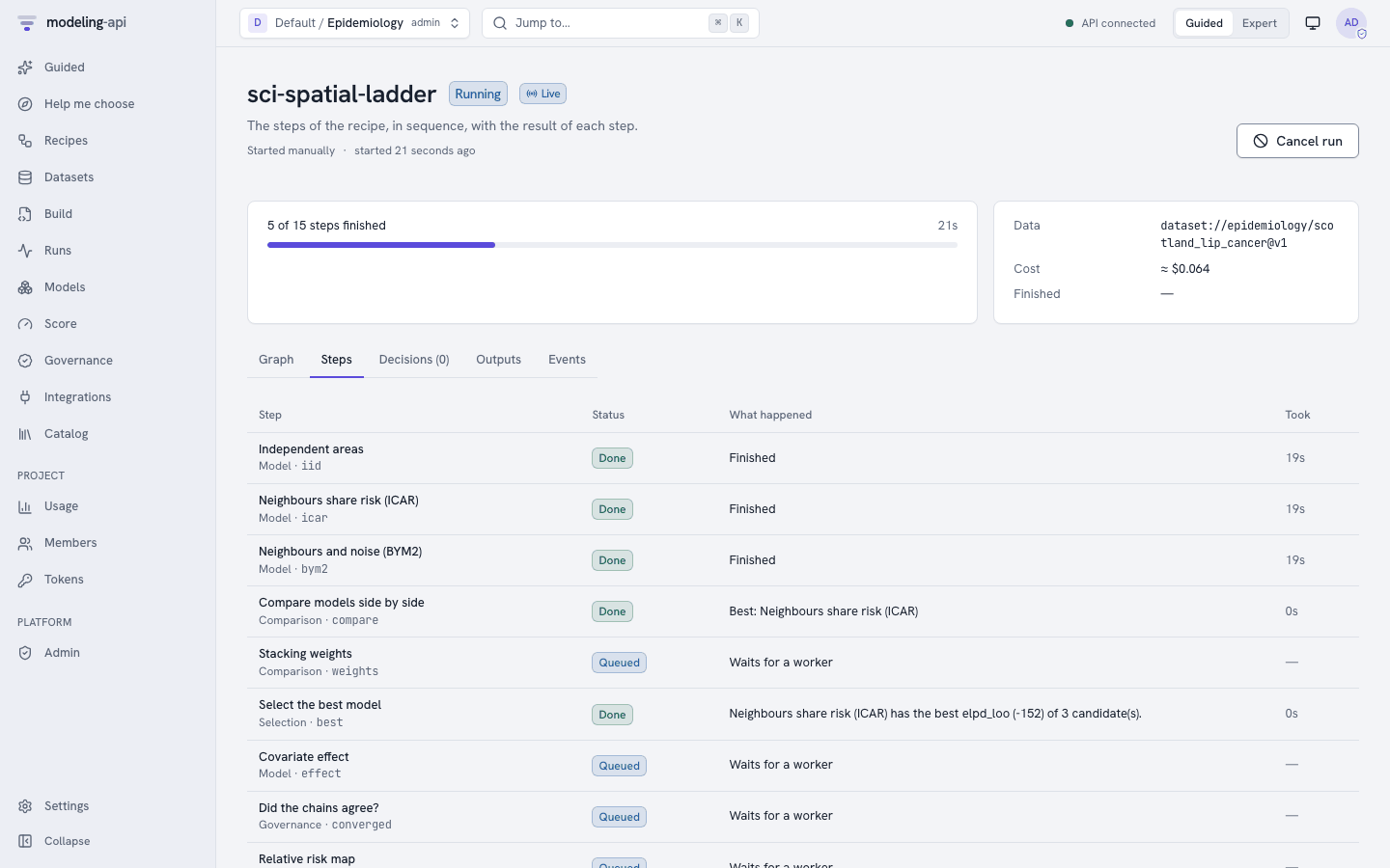
The Outputs tab shows the report of the run. It has the comparison table, the stacking weights, the effect of b1 with each prior width, the elpd_loo of each rung and the map of the best rung. The map of the recipe has no Observed smr panel.

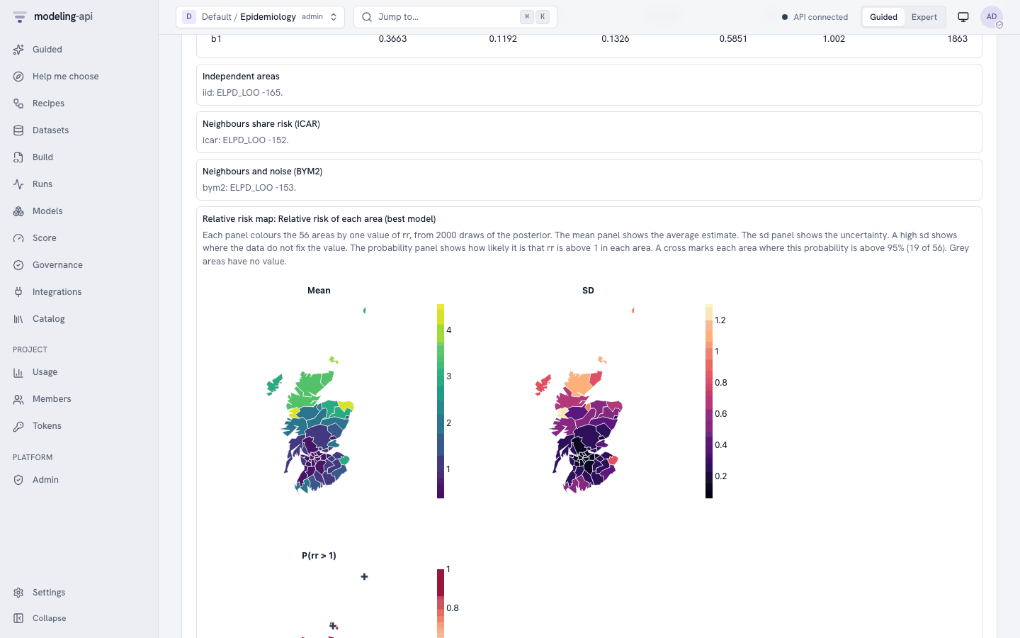
We ran the recipe on the exported data with engine: nutpie and the other defaults:

Node	Result
compare	The ranking is icar, bym2, iid. The best elpd_loo is −151.8
weights	The stacking weight of icar is 1.00. The pseudo-BMA weights are 0.67 (icar) and 0.33 (bym2)
best	"Neighbours share risk (ICAR) has the best elpd_loo (-152) of 3 candidate(s)."
effect	b1 0.379, 94% interval 0.148 to 0.625
clear	then: the chains agree and the range of b1 does not include zero
effect_wide, effect_narrow	b1 0.379 (0.139 to 0.627) and 0.366 (0.133 to 0.585)
converged	pass, R-hat 1.004

The recipe selects icar, not bym2. The notebook also found that the ICAR has the best elpd_loo (−151.9) and that the difference to BYM2 (0.8) is less than one standard error. The stacking weights put all the weight on one rung when the rungs are almost equal. Thus do not read the selection as "BYM2 is wrong". The notebook's decision to use BYM2 comes from its meaning, not from a difference in elpd. The b1 interval excludes zero with each prior width, so the association with AFF comes from the data, not from the priors.

Note

The default bind is {dims: {area: district, area_: district_}, vars: {covariate: aff}}. If your dataset has other names, change Bind in Fine-tune. For example, {"dims": {"area": "county", "area_": "county_"}, "vars": {"covariate": "smokers"}}.

The recipe bayes_workflow_audit (Bayesian workflow audit) also applies to this model. Type sci.areal_bym2@^1 in Model. In Fine-tune, type the bind above in Bind and {} in Prior predictive: the ICAR prior cannot give prior draws, and with prior draws the fit stops. The audit adds a posterior predictive check, a prior sensitivity check and a recovery check on simulated data. Its prior sensitivity check changes only prior widths with names such as prior_sigma. The prior widths of sci.areal_bym2 have other names (intercept_sd, slope_sd and sigma_scale), so this check is skipped. Thus the ladder recipe above fits the model again with these widths itself. The recovery check simulates the counts from the posterior predictive of the model, so each simulated dataset has whole counts.

9. The same with the CLI and the Python client

CLIPython

# get the data and the suggested spec
uv run python -m mapi_plugin_science.export e18 \
    --challenges <path to pymc-challenges>/data \
    --out scotland_lip.nc --spec scotland_lip.yaml

# upload, check and fit on the platform (scotland-lip-cancer-bym2.yaml is the spec of step 4)
mapi use <tenant>/epidemiology
mapi datasets upload scotland_lip.nc --name scotland_lip_cancer
mapi check scotland-lip-cancer-bym2.yaml --remote @
mapi fit scotland-lip-cancer-bym2.yaml --remote @
mapi explore model scotland-lip-cancer-bym2 -s params -s diagnostics

# the risk of each district (step 7)
cat > lip-score.yaml <<'EOF'
apiVersion: mapi/v1
kind: ScoreRequest
model: model://epidemiology/scotland-lip-cancer-bym2@latest
mode: predict
data: dataset://epidemiology/scotland_lip_cancer@latest
output: {kind: expected, summary: [mean, hdi_90], vars: [rr, p_exceed]}
seed: 1987
EOF
mapi score lip-score.yaml --remote @ --model <model id> --version 1 -o lip.zarr.zip

# the recipe (step 8)
mapi workflows init sci_spatial_ladder --name disease-map-ladder
mapi workflows apply disease-map-ladder.yaml
mapi workflows run disease-map-ladder \
    -i data=dataset://epidemiology/scotland_lip_cancer@latest \
    -p engine=nutpie --watch
RUN=$(mapi --json workflows runs disease-map-ladder -n 1 | jq -r '.[0].run_id')
mapi workflows node "$RUN" compare    # the rungs, best first
mapi workflows node "$RUN" weights    # the stacking weights
mapi workflows node "$RUN" clear      # is the effect of AFF clear?

The CLI has no models command. Take the model id from the run (mapi runs get <run>) or from Models in the web app.

from mapi_client import Client

api = Client()  # MAPI_URL, the `mapi login` sign-in (or MAPI_TOKEN) and MAPI_PROJECT

version = api.datasets.upload("scotland_lip.nc", dataset="scotland_lip_cancer")
print(version.ref, version.status.value)

with open("scotland-lip-cancer-bym2.yaml", encoding="utf-8") as fh:
    spec_yaml = fh.read()
check = api.specs.validate(spec_yaml)
print("valid" if check.valid else [(i.code, i.pointer) for i in check.issues])

revision = api.specs.upsert(spec_yaml)
run = api.runs.fit(revision.spec_id, revision.revision)
run = api.runs.wait(run.id, raise_on_failure=True)

model = next(m for m in api.models.list() if m.name == "scotland-lip-cancer-bym2")
mv = api.models.version(model.id, model.latest_version)
print(mv.ref, mv.metrics)

result = api.models.score(
    model.id,
    mv.version,
    {
        "model": mv.ref,
        "mode": "predict",
        "data": "dataset://epidemiology/scotland_lip_cancer@latest",
        "output": {
            "kind": "expected",
            "summary": ["mean", "hdi_90"],
            "vars": ["rr", "p_exceed"],
        },
        "seed": 1987,
    },
)
summary = result.tree["summary"]  # an xr.DataTree (needs the `xarray` extra)
p = summary["p_exceed"].sel(stat="mean")
print(int((p > 0.95).sum()), "districts with P(RR > 1) > 0.95")
print(summary["rr"].sel(stat="mean").to_series().nlargest(5))

workflow = api.workflows.create(template="sci_spatial_ladder")
wf_run = api.workflows.run(
    workflow.id,
    inputs={"data": "dataset://epidemiology/scotland_lip_cancer@latest"},
    params={"engine": "nutpie"},
    wait=True,
)
nodes = {n.node_id: n for n in wf_run.nodes}
print(nodes["compare"].result["ranking"])  # ['icar', 'bym2', 'iid']
print(nodes["effect"].result["params"]["b1"])

To compare with the notebook, load its printed posterior means with mapi_plugin_science.areal_data.challenges_reference().

The CLI and the client send the same spec and the same score request as the web app.

10. Differences from the notebook

The port keeps the likelihood, the five priors of the district effects, the scaling factor, the island links and the maps of notebook sections 3 to 7. It leaves out these parts:

• Other graphs (section 2). The export makes the queen graph only. In Python, areal_data.from_challenges(path, graph="rook") makes the rook graph, and graph="published" reads the hand-edited WinBUGS list. Write the result with write_export and upload it as a new dataset. This is "Try it yourself" item 2 of the notebook.
• Moran's I checks (sections 2 and 4). The fit keeps Moran's I of the log SMR on the linked graph (learned["morans_i_log_smr"], 0.53). The notebook uses the mainland graph and gets 0.50. The platform does not calculate Moran's I of the residual effects.
• The prior correlation against distance (section 3). Not in the platform.
• The isolated islands (failure 1). islands: isolate with kind: icar gives the "quiet" failure of the notebook: the islands get no information from other districts. kind: bym2 with islands: error gives the "loud" failure as SCHEMA_INVALID, and islands: isolate gives SETTINGS_INVALID.
• The unscaled BYM (failure 3). The platform has BYM2 only. It does not have separate priors on sigma_phi and sigma_theta.
• The shrinkage plot (section 7). Not in the platform. Compare the observed and the mean panels of the area map, or compare the rr of an iid fit and a bym2 fit.
• The 8-fold cross-validation (section 8). The platform holds out one block of 7 districts. To do more folds, fit the spec again with other values of split.seed.
• Restricted spatial regression (section 9). Not in the platform. The notebook also does not recommend it.

Next steps:

• Do "Try it yourself" item 3 of the notebook: put more prior weight on rho near 0, for example rho_alpha: 1 and rho_beta: 3. Do the data still move rho up?
• Compare BYM2 with a GP on the district centres. See the E07 tutorial for a GP on a grid.
• Read the model reference for the other science models.
• Read Workflows to change the ladder recipe.