E21 law-firm network latent space¶

This tutorial does the work of the pymc-challenges notebook E21_network_models.py in the web app. You use the model sci.network_latent_space@1. You do not write PyMC code.

You need:

The platform (start it with make dev) and a project that you can upload datasets to. This tutorial uses the project sociology. If your project has a different name, change the project part of each dataset:// and model:// reference, and metadata.project in the spec.
A local copy of pymc-challenges. The export command reads two files from its data/ directory.
About 20 minutes. Each fit takes less than one minute of sampler time.

1. The question¶

From 1988 to 1991, the sociologist Emmanuel Lazega studied a corporate law firm in New England. The firm had 71 lawyers (36 partners and 35 associates) in three offices: Boston, Hartford and Providence. Each lawyer marked the colleagues that they worked with in the last year. The network has a tie between two lawyers when they worked together. It has 378 ties in 2,485 pairs.

A pair of lawyers is a dyad. A logistic regression with one row for each dyad treats the 2,485 dyads as independent. They are not independent: each lawyer is in 70 dyads. A busy partner increases the tie probability of all 70 pairs. Two coworkers of one lawyer also work together much more often than two random lawyers.

The notebook asks these questions:

Do shared traits explain the ties? Same office, same practice, same status, same gender, same law school and the gap in years with the firm. (Notebook section 2, models a0 and a.)
What does a regression of independent dyads get wrong? (Section 2, model b with a sociality effect for each lawyer.)
Who works with whom, after the traits? A latent space gives each lawyer a position on a hidden map. (Section 3, model c, and the Procrustes alignment.)
Does the model make networks like the real one? (Section 5, the posterior predictive checks of the whole graph.)
Which model predicts the ties best? (Section 6, leave-one-dyad-out LOO.)

The notebook ends with this decision. Most of the network comes from homophily on office and practice and from the different activity of each lawyer (sociality). The latent space adds almost nothing to the prediction when the model has the traits and the sociality. Use the sociality model to measure the effects of the traits. Use the latent space to find structure that the traits do not show, and as a check that nothing large is missing.

What you will get, and the notebook section that each item replaces:

In the web app	Notebook
The effect of each shared trait, `sigma_s` and `sigma_z` (Parameters, `core.posterior_forest`)	Section 2, the table of the homophily effects, and section 3
The tie probability of each pair, with mean, sd and draws (Fields, `sci.field_map`)	Section 3, the tie probabilities of model c
The network on the latent map, coloured by office, with the observed ties (`net.graph`)	Section 3, the latent map
Convergence on the aligned positions (Diagnostics, `core.convergence`)	Section 3, the r_hat before and after Procrustes
`elpd_loo` of each kind (Metrics, and the recipe `sci_network_ladder`)	Section 6, the LOO table
Simulated networks and their statistics (Score, mode Simulate, `graph_stat`)	Section 5, the table of the graph statistics

See Differences from the notebook for the parts that the port leaves out. The block models of section 4 are one of them.

2. Get the data¶

The export command reads lazega_cowork.txt (the 71 × 71 table of ties) and lazega_attributes.txt (the traits of each lawyer). It makes the six pair covariates of the notebook. Run the command from the root of the modeling-api repository:

uv run python -m mapi_plugin_science.export e21 \
    --challenges <path to pymc-challenges>/data \
    --out lazega_coworkers.nc --spec lazega_coworkers.yaml

The command writes:

wrote lazega_coworkers.nc (variables cowork, homophily, office on lawyer=71, lawyer_=71, covariate=6)
upload it as dataset sociology/lazega_coworkers and fit sci.network_latent_space
wrote the suggested spec to lazega_coworkers.yaml

The file holds one dataset:

Name	Dims	Type	Meaning
`lawyer`	71	integer, policy `fixed`	The lawyers, 1 to 71. Lawyers 1 to 36 are partners
`lawyer_`	71	integer, policy `fixed`	The second lawyer of a pair, with the same labels
`covariate`	6	categorical, policy `fixed`	`same_office`, `same_practice`, `same_status`, `same_gender`, `same_school`, `years_gap`
`cowork`	`lawyer, lawyer_`	float64, target, missing values allowed	1 when the two lawyers worked together, else 0. The table is symmetric, and the diagonal is 0
`homophily`	`lawyer, lawyer_, covariate`	float64, covariate	1 when the two lawyers share the trait, else 0. `years_gap` is the gap in years with the firm ÷ 10
`office`	`lawyer`	int64, constant	The office: 1 Boston (48 lawyers), 2 Hartford (19), 3 Providence (4)

The dataset has no missing ties. The degree (the number of coworkers) of a lawyer is from 0 to 28. Lawyer 8 has no tie. The attribute mapi_schema gives each variable its role, so you do not map columns.

No pymc-challenges copy?

--synthetic writes a network that the model's own process simulates: 30 nodes in three offices, with three covariates (same_office, same_practice and years_gap) and known parameters. Use it to try the steps. The numbers in this tutorial are for the law firm.

uv run python -m mapi_plugin_science.export e21 --synthetic --out coworkers_synthetic.nc

3. Upload the dataset¶

Open Datasets in the sidebar.
Click New dataset.
Type lazega_coworkers in Name. Type a description, for example "Coworker ties of the 71 lawyers of the Lazega law firm".
Click Create dataset. The upload panel opens.
Click Choose files and select lazega_coworkers.nc.
Make sure that the format is netCDF (or HDF5 written by xarray).
Optional: click Preview structure. The panel shows Structure of the file. Make sure that it shows cowork on lawyer and lawyer_, homophily on three dims, and office on lawyer.
Optional: type a message in Version message (optional).
Click Upload and ingest.

The ingest run reads the file in the sandbox. When it is done, the version page shows the tabs Schema, Coordinates, Missingness, Preview and About. On Schema, cowork has the role target, homophily has the role covariate and office has the role constant.

The file is one plain dataset. You do not need the tree fields ("Put this file in a node of a tree (optional)") or the HDF5 path.

3.1 Explore the data¶

Look at the data before you build the spec.

On the version page, click Explore this version. The Data Explorer opens. The sections under Pictures of the data come first.
Click Network.
The first entry shows cowork, the ties between the 71 lawyers. The matrix puts similar lawyers next to each other. The node-link graph gives each office a colour.
The table of homophily gives the fraction of ties in the same office, and the fraction that you expect by chance. A much larger fraction shows that the office explains many ties.
The second entry shows homophily: one matrix for each of the 6 covariates (same_office, same_practice and the other covariates).
Group comparison and the time sections are in Not for this data.

Refer to Scientific data.

4. Build the spec¶

Open Build and click New spec. The editor opens with the geo MMM template.
Set the Editor view to YAML.
Open the Insert panel on the right.
Open the Datasets section and select lazega_coworkers. The toast "Dataset set" shows.
Type network in the search field. Under Models, select Who works with whom in a network (sci.network_latent_space@^1). The toast "Model set" shows.
Select all the text in the editor and paste the full spec below. The template has other blocks (a pipeline, a split and the MMM plots), so the spec must replace all of it.
Click Validate. The status shows valid.
Click Save spec. The spec gets its name lazega-coworkers-latent-space from metadata.name.

This is the full spec:

apiVersion: mapi/v1
kind: ModelSpec
metadata: {name: lazega-coworkers-latent-space, project: sociology}
data:
  dataset: dataset://sociology/lazega_coworkers@latest
  bind:
    dims: {node: lawyer, node_: lawyer_, cov: covariate}
    vars: {tie: cowork, dyad_cov: homophily, node_group: office}
model:
  use: sci.network_latent_space@^1
  settings: {kind: latent_space, covariates: true, node_groups: true, latent_dims: 2}
  fit: {mode: train_only, seed: 1991, tune: 2000, draws: 1000, chains: 4,
        target_accept: 0.95, engine: nutpie}
evaluate: {metrics: [elpd_loo]}
outputs:
  plots: [core.convergence, core.posterior_forest, net.graph, sci.field_map]

The model calls the nodes node and node_, the covariate dim cov, the target tie, the pair covariates dyad_cov and the group code node_group. The bind block connects them to the names in the dataset.

The spec has no split. The fit uses all 2,485 dyads, as the notebook does in sections 2 to 5. elpd_loo is leave-one-dyad-out: the model keeps the log-likelihood of each dyad. The suggested spec of the export (lazega_coworkers.yaml) is the same spec with tune: 1000 and without target_accept.

The settings for this question:

Setting	Value	What it means here
`kind`	`latent_space`	The log odds of a tie add the pair covariates, a sociality effect for each lawyer (`s_i + s_j`) and minus the distance between the two positions on the hidden map. This is model c of the notebook. `sociality` is model b, and `covariates` is model a
`covariates`	true	Use the six shared traits in `homophily`. With `false`, the model has no traits. `kind: covariates` with `covariates: false` is the Erdős-Rényi graph (model a0). `kind: latent_space` with `covariates: false` is model c0
`node_groups`	true	The dataset has `office`. The plots colour the lawyers by office
`latent_dims`	2 (default)	The dimensions of the hidden map. The notebook uses 2
`alpha_mu`, `alpha_sigma`	-2, 2 (default)	The normal prior of the intercept. It puts the density between about 1% and 50%
`beta_sigma`	1 (default)	The prior sd of each trait effect. A shared trait can multiply the odds by up to about 7, or divide them by 7
`sociality_scale`	1 (default)	The half-normal scale of `sigma_s`, the sd of the sociality effects
`latent_scale`	2 (default)	The half-normal scale of `sigma_z`, the spread of the positions on the map
`procrustes_iters`	10 (default)	The passes of the Procrustes alignment after the fit

The fit block uses tune: 2000 and target_accept: 0.95. The scale sigma_z of the hidden map mixes slowly when the model has the covariates. The notebook also reports this. More warm-up steps and smaller steps make the fit more stable. They do not remove the problem.

Why the positions converge

The distances do not change when the map turns, flips or moves. Thus the raw positions z_raw of the sampler do not converge, but each distance converges. After the fit, the model turns each draw onto one reference map (Procrustes analysis). The posterior keeps only the aligned position. The convergence check then uses only quantities that the data identify.

5. Fit and watch the run¶

Click Fit. The app opens the run page.
The badge shows Live while the run sends events.
The Progress card shows the progress of the sampler. The Events card shows the stages of the run and, at the end, the diagnostics. The Logs card stays empty when the model writes no output.
When the run is done, the Result card shows Inspect model://sociology/lazega-coworkers-latent-space@v1. Click it.

In our test, the fit took about 40 s with nutpie. After the fit, the run aligns the positions, calculates the tie probability of each pair for each draw, the plots and the explorer views.

You can also find the run under Runs. Filter it with the kind fit.

6. Read the result¶

On the model version page, the tabs are Overview, Diagnostics, Plots, Data tree, Preprocessing and Provenance. Click Explore to open the Model Explorer.

6.1 Can you trust the fit?¶

Open Diagnostics in the Model Explorer, or the plot Sampler convergence on the Plots tab. In our fit, 3 of the 2,000 checked parameters do not pass: sigma_z, alpha and one coordinate of one position. The largest R-hat is 1.015 (sigma_z), and the bulk ESS of sigma_z is about 140. There are no divergent transitions. The trait effects have R-hat below 1.003 and an ESS of more than 1,800.

This agrees with the notebook. sigma_z is wide and mixes slowly when the traits are in the model, because what is left for the map is a weak signal. Trust the trait effects and the tie probabilities. Do not report sigma_z to two digits.

Use more draws if the warning is larger

If R-hat of sigma_z is more than 1.05, set draws: 2000 and fit again. The sampler is random, so a second fit can show a larger warning than ours. With tune: 1000, one of our fits had R-hat 1.08 and 4 divergent transitions.

6.2 Do shared traits explain the ties?¶

Open Parameters in the Model Explorer, or the plot Posterior forest on the Plots tab. Each trait has one row beta[<trait>]. A positive value makes a tie more probable. In our fit, the posterior means and the 94% HDIs are:

Effect	Mean	94% HDI
`beta[same_office]`	2.55	2.22 to 2.89
`beta[same_practice]`	2.08	1.82 to 2.39
`beta[same_status]`	-0.60	-0.92 to -0.30
`beta[same_gender]`	0.39	0.10 to 0.73
`beta[same_school]`	0.33	0.08 to 0.58
`beta[years_gap]`	0.21	-0.01 to 0.42
`sigma_s`	0.90
`sigma_z`	0.92

Read the table as the notebook does:

Two lawyers in the same office have about e^2.5 ≈ 13 times the odds of a tie. The same practice multiplies the odds by about 8.
Two partners, or two associates, work together less often than a partner and an associate. The firm works in teams of partners and associates.
sigma_s ≈ 0.9: a lawyer one sd above the average has about e^0.9 ≈ 2.5 times the odds of a tie with anyone.

The rows sociality[<lawyer>] give the activity of each lawyer after the traits. In our fit, lawyer 15 has the highest sociality (2.1) and lawyer 8, who has no tie, has the lowest (-1.9). Lawyer 22 has the most ties (28), but a lower sociality (1.3), because the traits explain part of these ties.

6.3 The tie probability of each pair¶

Open Fields in the Model Explorer. The model has 1 output on a grid: tie_prob, the probability of a tie between two lawyers. The rows are lawyer and the columns are lawyer_. The diagonal is 0.

Select Mean in Statistic. A bright cell is a pair that probably works together.
Select Std. dev. to see where you are not sure of the probability.
Select Draws and click Play the draws to see possible tables that agree with the data.
Move the pointer over a cell to read its values. For example, the pair of lawyers 15 and 28 has a mean of about 0.66, and the pair of lawyers 1 and 8 has 0.02.

The lawyers are in the order of their numbers, so partners (1 to 36) are at the top and the left. Blocks of bright cells show the offices and the practices. The plot Field map of tie_prob on the Plots tab shows the same output as two panels (mean and sd).

6.4 The latent map¶

Open the plot Network of tie_prob (net.graph) on the Plots tab.

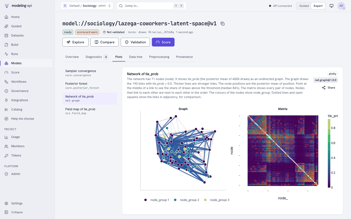
The plot Network of tie_prob: the 71 lawyers on the latent map, coloured by office, next to the matrix of the tie probabilities

The node positions are the posterior mean of position, the aligned map.
The colour of a node is its office.
A solid line is a pair with a mean tie_prob above 0.5. In our fit, 190 pairs pass. Thicker lines are more probable ties. Point at the middle of a line to see the share of the draws above 0.5.
Dotted lines show the observed ties (378), for comparison.
The matrix panel shows each pair. Lawyers that link to each other are next to each other.

In this model, the map shows only what the traits do not explain. Thus the offices and the practices are mixed on the map: the centres of the six groups (office × practice) are all within 0.4 of the middle. The direction of the map has no meaning: it is the direction of the Procrustes reference.

To see what the map finds without the traits (notebook model c0), fit the spec again with covariates: false. Then the plot shows these features, as in the notebook:

The four groups of Boston and Hartford (litigation and corporate in each office) are in four different areas of the map.
The 3 Providence corporate lawyers are near the Boston corporate lawyers.
sigma_z is about 2.3, not 0.9.

The model c0 was told nothing about the offices, but it finds them. Most of what the map finds alone is office and practice.

6.5 What a regression of independent dyads gets wrong¶

Fit the spec two more times to get models a and b of the notebook:

In Build, open the spec lazega-coworkers-latent-space.
Change kind: latent_space to kind: sociality.
Click Validate, then Save revision, then Fit.
Do steps 2 and 3 again with kind: covariates.

Each fit makes a new version of the model. Compare the trait effects in Parameters:

Effect	`covariates` (model a)	`sociality` (model b)
`beta[same_office]`	1.61 (89%: 1.39 to 1.84)	2.44 (89%: 2.14 to 2.74)
`beta[same_practice]`	1.59 (89%: 1.38 to 1.81)	2.01 (89%: 1.76 to 2.26)
`beta[same_status]`	-0.50	-0.54

The intervals of the office effect do not overlap. Model a is wrong with confidence, in two ways:

Attenuation. A logistic model without the sociality effects moves the effects toward zero. The busy partners, who work with everyone, make the contrast between the offices smaller.
Pseudo-replication. Model a thinks that it has 2,485 independent observations. Its intervals are too narrow.

6.6 Which model predicts the ties best?¶

The Metrics card of the Overview tab shows elpd_loo of each version. A larger value is better. The recipe of step 8 makes the same comparison in one run.

Model	Notebook	This port
a0, Erdős-Rényi (`kind: covariates`, `covariates: false`)	-1060.5	-1060.5
a, covariates (`kind: covariates`)	-894.2	-894.3
b, sociality (`kind: sociality`)	-763.4	-763.7
c0, latent space without covariates (`kind: latent_space`, `covariates: false`)	-795.7	-796.2
c, latent space (`kind: latent_space`)	-761.6	-761.0

The fit of c0 shows the warning PARETO_K_HIGH: for 7 dyads, the LOO estimate is not reliable. The notebook also finds such dyads for c0.

The difference between c and b is about 2.7, and its standard error is about 2.6. (We calculated the standard error with ArviZ az.compare on the two fits. The web app does not show it.) A difference of about one standard error is not a real difference: the two models are equal. Both models are far better than model a, which has no sociality.

6.7 The numbers of the notebook and of this port¶

Quantity (model c)	Notebook	This port
`beta[same_office]`	2.54	2.55
`beta[same_practice]`	2.08	2.08
`beta[same_status]`	-0.59	-0.60
`beta[same_gender]`	0.38	0.39
`beta[same_school]`	0.33	0.33
`beta[years_gap]`	0.21	0.21
`sigma_s`	0.90	0.90
`sigma_z`	0.88	0.92 (sd 0.29)
`elpd_loo`	-761.6	-761.0

Your numbers can be slightly different if the sampler or its version is different. sigma_z changes most from one fit to the next.

6.8 Make the decision¶

Use these outputs to make the decisions of the notebook:

Do not use a regression of independent dyads. Compare the trait effects of covariates and sociality (section 6.5). If they are different, the sociality is necessary.
Choose the model for the trait effects. Compare elpd_loo (section 6.6). If the latent space is better by less than two standard errors, use the simpler sociality model to report the effects. For the law firm, the two models give the same effects to two digits.
Use the latent space to find structure. Fit latent_space with covariates: false and look at the map in Network of tie_prob. If the map shows groups that you know (the offices, the practices), the traits that you have capture the structure. A group that no trait explains is a reason to look for a new trait.
Do a check of the whole graph. Simulate networks (step 7.2) and compare their statistics with the real network. A statistic far outside the simulations shows what the model does not make.

7. Score the model¶

A score needs a dataset with the dims lawyer and lawyer_, and homophily for each pair. Send the dataset that you fitted. The node set is fixed: a lawyer that the fit did not see stops the score with UNSEEN_LEVELS.

7.1 Predict: the tie probabilities and the degrees¶

On the model version page of lazega-coworkers-latent-space, click Score.
In What do you want to do?, select Predict.
In Values to score, select Use a dataset. Select lazega_coworkers.
Open Advanced. Set Seed (optional) to 21. Type tie_prob, degree, sociality in Variables (optional).
Click Predict.

The request that the page sends (POST /v1/models/{model_id}/versions/{v}:score) is:

{
  "apiVersion": "mapi/v1",
  "kind": "ScoreRequest",
  "model": "model://sociology/lazega-coworkers-latent-space@latest",
  "mode": "predict",
  "data": "dataset://sociology/lazega_coworkers@latest",
  "output": {
    "kind": "expected",
    "summary": ["mean", "hdi_90"],
    "vars": ["tie_prob", "degree", "sociality"]
  },
  "seed": 21
}

The result has tie_prob(lawyer, lawyer_), degree(lawyer) (the expected number of coworkers) and sociality(lawyer). In our fit, half of the sum of the expected degrees is 378.5. The network has 378 ties. Lawyer 22 has the largest expected degree (26.3).

To score a part of the firm, send a dataset with fewer lawyers. degree then counts only the ties inside that part.

7.2 Simulate: networks for a check of the whole graph¶

In What do you want to do?, select Simulate.
In Values to score, select Use a dataset. Select lazega_coworkers.
Open Advanced. Set Quantity to Predictive. Set Draws to 500.
Type graph_stat, degree in Variables (optional).
Click Simulate.

{
  "apiVersion": "mapi/v1",
  "kind": "ScoreRequest",
  "model": "model://sociology/lazega-coworkers-latent-space@latest",
  "mode": "simulate",
  "data": "dataset://sociology/lazega_coworkers@latest",
  "output": {
    "kind": "predictive",
    "summary": ["mean", "hdi_90"],
    "draws": 500,
    "vars": ["graph_stat", "degree"]
  },
  "seed": 21
}

Each draw is one simulated network of the 71 lawyers. graph_stat(statistic) gives nine statistics of each network. Compare them with the real network:

Statistic	Real network	Simulated, mean	Simulated, 90% HDI
`density`	0.152	0.152	0.138 to 0.165
`sd_degree`	5.74	5.93	5.25 to 6.66
`max_degree`	28	29.4	24 to 34
`isolates`	1	0.32	0 to 1
`triangles`	493	485	364 to 608
`transitivity`	0.307	0.294	0.261 to 0.325
`esp0`	12	23.5	12 to 33
`mean_geodesic`	2.10	2.11	2.04 to 2.19
`unreachable`	0.028	0.009	0 to 0.028

The web app does not calculate the statistics of the real network. The values in the second column are from the notebook's functions.

The model makes the spread of the degrees and the transitivity of the real network.
esp0 is the number of ties whose two lawyers have no coworker in common. The real network has 12. In our simulations, 97% of the networks have 12 or more. As in the notebook, the real collaboration is more closed than the model makes.
The real network has one isolate (lawyer 8). The simulations have fewer.

Send all the lawyers for graph_stat

Send a dataset with all 71 lawyers in lawyer and lawyer_, and use Simulate or Predictive. Otherwise the score stops with CAPABILITY_UNSUPPORTED. A statistic of the whole graph needs the whole graph.

If you promote the version to an endpoint, Integrations → the endpoint → Schema and Try it sends the same requests.

8. Run a workflow recipe¶

8.1 The network ladder¶

The recipe sci_network_ladder ("Network ties: which model?") does sections 2, 3, 5 and 6 of the notebook in one run:

It fits the three kinds covariates, sociality and latent_space on the same dyads.
It ranks them by elpd_loo (node compare) and calculates their stacking weights (node weights).
It keeps the model with the best elpd_loo (node best).
It shows alpha and the trait effects of that model (node effects).
It draws the network with net.graph (node graph).
It simulates networks from that model (node simulate) and plots the spread of their density and transitivity with core.ridge (node ppc).
It writes a report.

The defaults of the recipe fit the dataset of the e21 export. You do not change the binding.

Set the header to Guided and open Recipes. In Expert mode, open Workflows and the Templates tab.
Find the card Network ties: which model? and click Run on my data.
In 1. Your data, select lazega_coworkers in Dataset.
Open Fine-tune (optional: the defaults are correct for most data). Set Engine to nutpie. Set Tune to 2000 and Target accept to 0.95, as in step 4.
Click Run this recipe.

The monitor of the run has the tabs Graph, Steps, Decisions, Outputs and Events. Outputs has the comparison table, the stacking weights, the effects, the network plot, the plot of the simulated statistics and the report.

What to look for:

The comparison table ranks latent_space first, sociality second and covariates last.
The stacking weights put most of the weight on latent_space. In our fits with ArviZ, the weights are about 0.91, 0.08 and 0.01.
best selects latent_space, because it has the largest elpd_loo.

The best rung is not always the model to report

select.best uses only the value of elpd_loo. It does not use the standard error of the difference. For the law firm, the difference between latent_space and sociality is about one standard error (section 6.6). Read the table before you report the effects of best. The notebook reports the sociality model.

Note

The recipe fits the model three times and simulates 500 networks. With nutpie, the run takes a few minutes. With the default engine pymc, it takes longer.

8.2 Other recipes¶

bayes_workflow_audit ("Bayesian workflow audit") does the checks of a Bayesian workflow on one model. In 2. What the recipe needs to know, type sci.network_latent_space@^1 in Model. In Fine-tune, type {"kind": "sociality", "node_groups": true} in Settings and the bind of step 4 as JSON in Bind. The recovery check simulates each graph from the posterior predictive of the model, so each tie is 0 or 1. It fits the model many times, so it takes longer.
sci_spatial_ladder, sci_phylo_signal, sci_calibrate_then_design and sci_image_model_check are for other science models. They do not apply to this model.

9. The same with the CLI and the Python client¶

CLIPython

mapi use <tenant>/sociology
mapi datasets upload lazega_coworkers.nc --name lazega_coworkers
mapi check lazega-coworkers-latent-space.yaml --remote @   # the server's static validation
mapi fit lazega-coworkers-latent-space.yaml --remote @     # create or revise the spec, fit, follow
mapi explore model lazega-coworkers-latent-space -s params -s diagnostics

cat > simulate-networks.yaml <<'EOF'
apiVersion: mapi/v1
kind: ScoreRequest
model: model://sociology/lazega-coworkers-latent-space@latest
mode: simulate
data: dataset://sociology/lazega_coworkers@latest
output: {kind: predictive, summary: [mean, hdi_90], draws: 500, vars: [graph_stat, degree]}
seed: 21
EOF
mapi score simulate-networks.yaml --remote @ --model <model id> --version 1 \
  -o simulate-networks.zarr.zip

mapi workflows init sci_network_ladder --name coworker-ladder   # writes coworker-ladder.yaml
mapi workflows apply coworker-ladder.yaml
mapi workflows run coworker-ladder \
  -i data=dataset://sociology/lazega_coworkers@latest \
  -p engine=nutpie -p tune=2000 -p target_accept=0.95 --watch
RUN=$(mapi --json workflows runs coworker-ladder -n 1 | jq -r '.[0].run_id')
mapi workflows node "$RUN" compare    # the kinds, best first
mapi workflows node "$RUN" effects    # alpha and beta[...] of the best kind
mapi workflows output "$RUN" simulate scores --out graph_stats.zarr.zip

lazega-coworkers-latent-space.yaml is the spec of step 4. The CLI has no models command. Take the model id from the run (mapi runs get <run>) or from Models in the web app.

from mapi_client import Client

api = Client(project="<tenant>/sociology")
version = api.datasets.upload("lazega_coworkers.nc", dataset="lazega_coworkers")
print(version.ref, version.status.value)

with open("lazega-coworkers-latent-space.yaml", encoding="utf-8") as fh:
    spec_yaml = fh.read()
check = api.specs.validate(spec_yaml)
print("valid" if check.valid else [(i.code, i.pointer) for i in check.issues])
revision = api.specs.upsert(spec_yaml)
run = api.runs.fit(revision.spec_id, revision.revision)
run = api.runs.wait(run.id, raise_on_failure=True)

model = next(m for m in api.models.list() if m.name == "lazega-coworkers-latent-space")
result = api.models.score(
    model.id,
    model.latest_version,
    {
        "model": "model://sociology/lazega-coworkers-latent-space@latest",
        "mode": "simulate",
        "data": "dataset://sociology/lazega_coworkers@latest",
        "output": {
            "kind": "predictive",
            "summary": ["mean", "hdi_90"],
            "draws": 500,
            "vars": ["graph_stat"],
        },
        "seed": 21,
    },
)
summary = result.tree["summary"]  # an xr.DataTree (needs the `xarray` extra)
print(summary["graph_stat"].sel(stat="mean").to_series())

workflow = api.workflows.create(template="sci_network_ladder")
ladder = api.workflows.run(
    workflow.id,
    inputs={"data": "dataset://sociology/lazega_coworkers@latest"},
    params={"engine": "nutpie", "tune": 2000, "target_accept": 0.95},
    wait=True,
)
nodes = {n.node_id: n for n in ladder.nodes}
print(nodes["best"].result["reason_plain"])
print(nodes["effects"].result["params"]["beta[same_office]"])

10. Differences from the notebook¶

The port keeps the models a0, a, b, c and c0 of sections 2 and 3 and the Procrustes alignment. It also keeps the latent map, the graph checks of section 5 and the leave-one-dyad-out LOO of section 6. It leaves out these parts:

The block models (section 4). The port has no stochastic block model and no mixed-membership block model. Thus it does not give the probability that two lawyers are in the same block.
The held-out split with AUC (section 6). The port has no AUC metric and no ROC curve. A mask_block split over [node, node_] holds out random cells, and a dyad is out of the fit when one of its two cells is out. The metrics of such a split count the diagonal cells, so use elpd_loo to compare the kinds.
The figures of the raw positions (section 3). The port aligns the positions after each fit. It does not show the turn of the map within a chain, or the r_hat of the raw positions.
The details of the latent map. net.graph shows the mean positions coloured by office. It does not draw a 50% ellipse for each lawyer or a marker for the practice. Calculate them from the draws of position.
The full histograms (section 5). graph_stat gives esp0 and mean_geodesic, not the full distributions of the shared partners and of the geodesics.
The statistics of the real network. The web app does not calculate them. Use graph_stats from mapi_plugin_science.network on cowork in Python.
Directed ties ("Try it yourself", friendship). The model accepts only a symmetric table.

Next steps:

Fit latent_space with covariates: false and compare its map with the offices and the practices.
Fit latent_dims: 3 and compare elpd_loo.
Read the workflow cookbook to change the network ladder.
Read the model reference for the other science models.