05 · The apps from a notebook

You will learn

• Read a model's estimand in words and plot its curves with their band
• Optimise a budget with an interval and P(beats plan), nothing saved
• Rank what to test next by EIG and EVOI

You need

• Nothing to read it; rerunning needs the reference deployment with its apps, seeded

Run this notebook Recorded session

notebooks/05_apps_from_a_notebook.ipynb

A recorded session against the reference deployment. It cannot be run without that deployment; the outputs on this page were saved from that session.

About 20 minutes

Access needed. The packages and notebooks are not yet publicly distributed. The steps below need a checkout of the UMP repository. Pages show recorded outputs, so you can follow along without running them.

Recorded run

This page shows a recorded session against the reference deployment. It cannot be run without that deployment. The identity stub (as_=) and the localhost address belong to the reference deployment, not to the standard; a conforming core authenticates callers as section 19 requires.

The web front end is one way into the apps; a notebook is another.

The media lead’s question, Monday morning: should Northwind move money, and by how much? Priya answers it from her notebook with the same services the web app calls:

1. engines: which modelling engines are live and what they can do;
2. models: the validated model, what its numbers mean, its response curves with their band;
3. planner: the budget optimised on that model, with intervals and P(beats plan); nothing saved;
4. experiments: which channel is worth testing next;
5. console: where the client stands.

Writes: step 4 stores one priority snapshot in the experiments app. Everything else only reads.

In [1]:

import os

import babelfin as fin

CLIENT = os.environ.get("UMP_NOTEBOOK_CLIENT", "northwind-e2e-live")
s = fin.connect(as_="maya.chen")

1. Engines

Engines run behind adapters, each in its own container with its own lockfile; the core never imports a modelling library.

In [2]:

s.engines()[["name", "kind", "family", "reachable", "stub", "tiers_produced"]]

Out [2]:

	name	kind	family	reachable	stub	tiers_produced
0	atlas-planner	planner	media_mix	True	False	[]
1	geo-experiments	experiment	media_mix	True	False	[]
2	mapi-mmm	model	media_mix	True	False	[A, C]
3	mei	model	effectiveness_index	True	False	[B]
4	an in-house MMM framework	model	media_mix	True	False	[A, B, C, D]
5	mtm-negative-control	negative_control	media_tracking	True	False	[D]

2. The model and its curves

In [3]:

s.models.list(client=CLIENT, state="validated", tier="A")

Out [3]:

	id	title	state	tier	engine	capability_status
0	mdl_d6b843bfde3848f2886d	Northwind MMM (Bayesian NUTS) [northwind-e2e-l...	validated	A	an in-house MMM framework	certified
1	mdl_a03aad21a7f6431c9709	Northwind MMM (Bayesian NUTS) [northwind-e2e-l...	validated	A	an in-house MMM framework	certified

In [4]:

model = s.models.get(s.models.list(client=CLIENT, state="validated", tier="A").iloc[0]["id"])
model

Out [4]:

Northwind MMM (Bayesian NUTS) [northwind-e2e-live] (calibrated R4)

A full model that passed the accuracy test; refit today.

details

id	mdl_d6b843bfde3848f2886d
tier	A
means	roi: revenue per dollar from removing all spend, geo_set, versus zero spend, over 104 weeks, posterior mean, 94% hdi
acceptance	passed
use	validated method
dependence	joint_draws

Response curves come on a spend grid (0 to 2.5 times current spend, the proposed Tier C grid). rung says which rung of the fallback ladder produced them, and the band says how it was drawn.

In [5]:

curves = model.curves()
curves

Out [5]:

<Curves 4 channels, 3 draws, spend_table, band min_max>

In [6]:

curves.plot();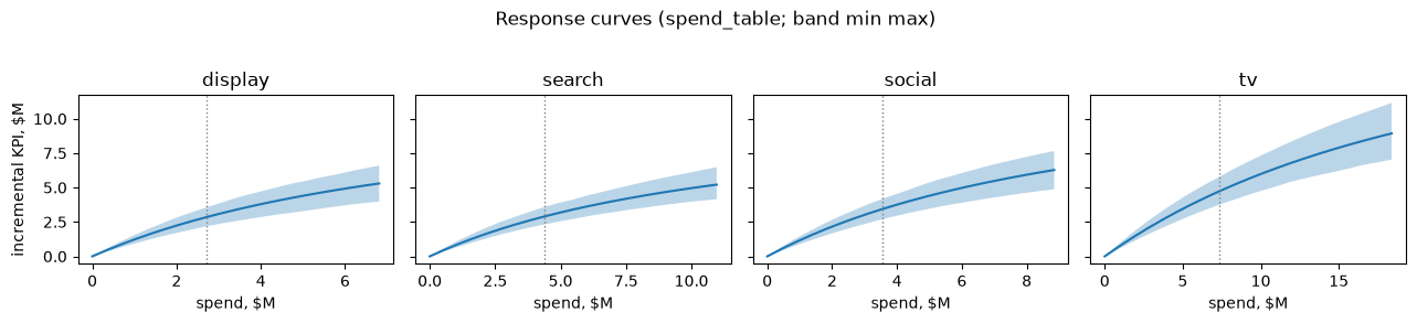

Out [6]:

3. Optimise the budget (nothing saved)

The planner optimises on the model’s joint draws. The uplift is a number with its own estimand: a reallocation against the current plan. opt.save("name") would save it as a scenario, the same as the web app’s Save button.

In [7]:

opt = s.planner.optimize(model, max_change=0.30)
opt

Out [7]:

Uplift vs current plan: 373,412, likely between $89K and $650K

engine budget_optimizer

details

means	revenue in total from moving 1,870,673 of spend from search, tv to display, social (total unchanged), versus the current plan, over 52 weeks, posterior mean, 90% eti
P(beats current plan)	0.985
ladder	full_model
dependence	joint_draws
saved	no (pass save=True or call .save(name))

channel	current_spend	optimal_spend	change_pct	interval_lo	interval_hi
display	2723561.0	3538441.0	30.0	3328406.0	3540629.0
search	4385998.0	3434452.0	-22.0	3070199.0	4713605.0
social	3537429.0	4593222.0	30.0	4033065.0	4598658.0
tv	7353012.0	6433885.0	-13.0	5147108.0	6887863.0

In [8]:

opt.allocation.to_frame().round(0)

Out [8]:

	channel	current_spend	optimal_spend	change_pct	interval_lo	interval_hi
0	display	2723561.0	3538441.0	30.0	3328406.0	3540629.0
1	search	4385998.0	3434452.0	-22.0	3070199.0	4713605.0
2	social	3537429.0	4593222.0	30.0	4033065.0	4598658.0
3	tv	7353012.0	6433885.0	-13.0	5147108.0	6887863.0

In [9]:

opt.uplift

Out [9]:

uplift in revenue versus the baseline plan (optimised_plan:budget_optimizer): 373,412

likely between $89K and $650K · low confidence

details

means	revenue in total from moving 1,870,673 of spend from search, tv to display, social (total unchanged), versus the current plan, over 52 weeks, posterior mean, 90% eti
interval	90% eti 89,339 to 650,251
trust level	2

4. What should we test next?

Candidate tests ranked by expected information gain and expected value of information, using the model’s posterior. The rule is stated, and no (1 - 1/e) greedy bound is claimed for EVOI.

In [10]:

priority = s.experiments.prioritise(model)
priority

Out [10]:

Test next: tv

keep the plan, or move 20% of one channel's spend to another; pick the action with the highest expected annual KPI

details

kept	P1
note	No (1 - 1/e) bound is claimed for EVOI or for budget-constrained selection. Keeping the better of P1 (cost-scaled greedy) and P2 (best single test) gives a constant-factor guarantee for EIG only.

channel	eig	evoi	cost	n_treated	n_markets	weeks	design
tv	0.0015	248.1330	75905.4678	10	50	6	randomised_geos
display	0.0007	233.5540	43855.4200	10	50	6	randomised_geos
social	0.0007	154.9855	49489.8944	10	50	6	randomised_geos
search	0.0005	115.7876	55364.6025	10	50	6	randomised_geos

In [11]:

priority.to_frame().round(4)

Out [11]:

	channel	eig	evoi	cost	n_treated	n_markets	weeks	design
0	tv	0.0015	248.1330	75905.4678	10	50	6	randomised_geos
1	display	0.0007	233.5540	43855.4200	10	50	6	randomised_geos
2	social	0.0007	154.9855	49489.8944	10	50	6	randomised_geos
3	search	0.0005	115.7876	55364.6025	10	50	6	randomised_geos

5. Where the client stands

The console’s client view: returns per channel with their source and interval. The same JSON feeds leadership’s Measurement Console.

In [12]:

view = s.console.client(CLIENT)
view.returns

Out [12]:

	channel	source	value	lo	hi	level	range_words	label
0	TV	best_guess	2.346911	1.266270	4.349775	0.95	likely between $1.27 and $4.35	TV return (benchmark best guess)
1	Search	best_guess	3.226087	1.503377	6.922840	0.95	likely between $1.50 and $6.92	Search return (benchmark best guess)
2	Social	best_guess	2.690645	1.571230	4.607581	0.95	likely between $1.57 and $4.61	Social return (benchmark best guess)
3	Display	not_available	NaN	NaN	NaN	NaN	NaN	NaN

In [13]:

s.close()

Going deeper

Every result keeps the app’s JSON on .raw, and each app’s OpenAPI page lists the rest (http://localhost:8104/docs for the planner, and so on). The rest of the Monday story (decision draft, review, Newton’s read-only drafts, the signature and the sealed decision) is in the reference deployment’s tooling.