11 · Conversion lift: ITT, CACE and why platform A/B never calibrates

You will learn

Plan a lift test with power and assurance
Tell intent-to-treat from the effect on the exposed (CACE)
Correct segment results for multiple tests with Benjamini-Hochberg
See a class D platform A/B test excluded from calibration

You need

Python 3.12 and uv
Notebook 01, or the estimand idea from it

Run this notebook Offline

notebooks/11_conversion_lift_itt_cace_ghost_ads.ipynb

Runs offline on your laptop. The outputs on this page were saved from a real run.

About 30 minutes

Access needed. The packages and notebooks are not yet publicly distributed. The steps below need a checkout of the UMP repository. Pages show recorded outputs, so you can follow along without running them.

cd notebooks && uv run jupyter lab

Runs offline. Uses babelfin, NumPy, pandas, SciPy and matplotlib. The data is SYNTHETIC, generated below with a known truth (TRUE), so every number can be checked.

Northwind Outdoor’s six-week YouTube flight has ended. Li Wei has two readouts on her desk and a budget meeting on Thursday. The platform’s “A/B creative test” says +18% conversions, and the CMO has already put that in a slide. The other readout is the ghost-ads user holdout the agency pre-registered. Its first number looks disappointingly small next to 18%.

This notebook is Li’s afternoon: plan, readout, a false start, the segment trap, and what UMP lets each number do.

In [1]:

import babelfin as fin
import matplotlib.pyplot as plt
import numpy as np
import pandas as pd
from scipy.stats import norm

SEED = 8
Z90 = norm.ppf(0.95)                              # every interval here is 90%, matching the estimands
pd.set_option("display.max_colwidth", None)       # an estimand is a sentence; never cut it short


def table(numbers):
    """A list of fin.Number as rows: value, interval and the estimand in words."""
    return pd.DataFrame([{"label": n.label, "value": n.value, "lo": n.lo, "hi": n.hi, "estimand": n.estimand.words}
                         for n in numbers]).round(2)

1. Two numbers on Li’s desk and the CMO’s 18%

The three estimands Li will hand over. Same KPI (conversions), same channel and window, different populations. Rates are tiny (0.4% is “big” here), so every rate is scaled per 1,000 users.

In [2]:

itt_e = fin.estimand("E-USER-ITT", kpi="conversions_per_1000_eligible_users", per="absolute", population="itt",
                     channels="youtube", weeks=6, level=0.9)
cace_e = fin.estimand("E-USER-ITT", kpi="conversions_per_1000_exposed_users", per="absolute", population="exposed",
                      channels="youtube", weeks=6, level=0.9)
iroas_e = fin.estimand("E-USER-ITT", kpi="revenue", per="spend", population="itt",
                       channels="youtube", weeks=6, level=0.9)
for e in (itt_e, cace_e, iroas_e):
    print("-", e.words)

Out [2]:

- conversions per 1000 eligible users in total, net from removing all spend, itt, versus the control counterfactual, over 6 weeks, estimator point, 90% confidence
- conversions per 1000 exposed users in total, net from removing all spend, exposed, versus the control counterfactual, over 6 weeks, estimator point, 90% confidence
- revenue per dollar, net from removing all spend, itt, versus the control counterfactual, over 6 weeks, estimator point, 90% confidence

2. Plan first: power and assurance

Three weeks before launch, the client asked for a 10% holdout (“we don’t want to lose 20% of the audience”). Li sized it with a normal approximation, with no simulation needed:

SE of CACE ≈ √(p(1−p)(1/n_t + 1/n_c)) ÷ exposure rate, at p = 2% and 35% expected reach.
Assurance is power averaged over what we believe the effect is. The belief came from the Tier D MMM’s YouTube summary, translated to about 5 per 1,000 exposed users, sd 1.5. That translation is an assumption.

In [3]:

PRIOR = {"mean": 5.0, "sd": 1.5}     # per 1,000 exposed users; ASSUMED, from the MMM's Tier D summary


def se_cace(n, treat_share, reach=0.35, p=0.02):
    """Normal-approximation SE of the Wald CACE, per 1,000 exposed users."""
    nt, nc = n * treat_share, n * (1 - treat_share)
    return 1000 * np.sqrt(p * (1 - p) * (1 / nt + 1 / nc)) / reach


def assurance(n, treat_share):
    s = se_cace(n, treat_share)
    d = np.random.default_rng(0).normal(PRIOR["mean"], PRIOR["sd"], 200_000)
    return float(np.mean(norm.cdf(d / s - Z90) + norm.cdf(-d / s - Z90)))


def mde80(n, treat_share):          # smallest effect detected with 80% power at the 90% level
    return (Z90 + norm.ppf(0.8)) * se_cace(n, treat_share)


plans = pd.DataFrame([{"holdout": f"{1 - s:.0%}", "SE per 1k exposed": se_cace(400_000, s),
                       "MDE80 per 1k exposed": mde80(400_000, s), "assurance": assurance(400_000, s)}
                      for s in (0.9, 0.8)]).round(2)
plans

Out [3]:

	holdout	SE per 1k exposed	MDE80 per 1k exposed	assurance
0	10%	2.11	5.24	0.72
1	20%	1.58	3.93	0.86

The 10% holdout gives about 72% assurance. UMP’s floor is 80% (proposed, §9). The plan goes through fin.check as a plain dict: babelfin has no TestPlan wrapper, so the dict is the document.

In [4]:

plan = {"client_id": "northwind-outdoor", "question": "Does YouTube drive incremental conversions?",
        "decision_informed": "Q1 YouTube budget", "channel": "youtube", "primary_metric": "conversions",
        "estimand": cace_e.to_dict(), "design": "ghost_ads", "estimator": "cace", "admissibility_class": "A",
        "power": {"assurance": round(assurance(400_000, 0.9), 2), "mde": round(mde80(400_000, 0.9), 2),
                  "duration_weeks": 6}}
fin.check("test_plan", plan).to_frame()

Out [4]:

	gate	outcome	message	codes
0	G-EXP-01	fallback	not pre-registered	NOT_PREREGISTERED
1	G-EXP-02	warn	assurance 72% is below the 80% proposed floor	LOW_ASSURANCE

Two gates fire, and neither blocks:

G-EXP-02 warns LOW_ASSURANCE.
G-EXP-01 falls back: the plan is not locked yet.

G-EXP-03, the spillover check, does not apply. Users are randomised one by one, so there are no neighbouring geos to leak into. Li takes the warning to the client and wins a 20% holdout. Then she locks the plan.

In [5]:

revised = {**plan, "power": {"assurance": round(assurance(400_000, 0.8), 2), "mde": round(mde80(400_000, 0.8), 2),
                             "duration_weeks": 6},
           "preregistration": {"locked": True, "primary_metric": "conversions", "analysis_method": "cace",
                               "decision_rule": "scale YouTube if the CACE 90% interval excludes 0"},
           "status": "locked"}
r = fin.check("test_plan", revised)
print(r, "| assurance", revised["power"]["assurance"])

Out [5]:

<GateReport Would pass · 0 stops · 0 fallbacks · 0 warnings · 12 gates (0 fired)> | assurance 0.86

3. Simulate the holdout, with ghost-ad flags

Each eligible user is randomised: 80% treat, 20% control. In treat, the ad server reaches 35% of users. In control the ads are suppressed, but the server logs a ghost ad wherever it would have served. Reached users are heavier converters to start with (3.6% vs 1.1%), which is why naive “exposed vs unexposed” comparisons lie.

Truth: +4.0 conversions per 1,000 exposed users, concentrated in the 25 to 34 band.

In [6]:

TRUE = {"n_eligible": 400_000, "treat_share": 0.8, "exposure_rate": 0.35, "base_cr": 0.020,
        "base_cr_reached": 0.036, "cace_abs_lift": 0.0040, "itt_abs_lift": 0.0014, "aov": 85.0, "spend": 24_000,
        "segment_share": {"18_24": 0.15, "25_34": 0.35, "35_54": 0.40, "55_plus": 0.10},
        "segment_cace": {"18_24": 0.0, "25_34": 0.0080, "35_54": 0.0030, "55_plus": 0.0},
        "platform_ab_selection_bias": 0.0026}
# The truth is internally consistent: segment lifts average to the overall CACE, ITT = CACE x reach.
assert np.isclose(sum(TRUE["segment_share"][s] * TRUE["segment_cace"][s] for s in TRUE["segment_cace"]),
                  TRUE["cace_abs_lift"])
assert np.isclose(TRUE["cace_abs_lift"] * TRUE["exposure_rate"], TRUE["itt_abs_lift"])
TRUE["iroas"] = TRUE["itt_abs_lift"] * TRUE["n_eligible"] * TRUE["treat_share"] * TRUE["aov"] / TRUE["spend"]


def simulate(seed=SEED):
    rng = np.random.default_rng(seed)
    n = TRUE["n_eligible"]
    segment = rng.choice(list(TRUE["segment_share"]), n, p=list(TRUE["segment_share"].values()))
    treat = rng.random(n) < TRUE["treat_share"]
    would_serve = rng.random(n) < TRUE["exposure_rate"]          # the ad server's choice, logged in both arms
    p_rest = (TRUE["base_cr"] - TRUE["exposure_rate"] * TRUE["base_cr_reached"]) / (1 - TRUE["exposure_rate"])
    lift = pd.Series(segment).map(TRUE["segment_cace"]).to_numpy()
    p = np.where(would_serve, TRUE["base_cr_reached"], p_rest) + (treat & would_serve) * lift
    return pd.DataFrame({"segment": segment, "treat": treat, "exposed": treat & would_serve,
                         "ghost": ~treat & would_serve, "converted": rng.random(n) < p})


users = simulate()
users.groupby("treat").agg(users=("converted", "size"), exposed=("exposed", "mean"), ghost=("ghost", "mean"),
                           conv_rate=("converted", "mean")).round(4)

Out [6]:

	users	exposed	ghost	conv_rate
treat
False	80039	0.0000	0.3519	0.0199
True	319961	0.3499	0.0000	0.0214

The ghost flag earns its keep before any lift is computed: control’s ghost rate matches treat’s exposure rate, so the ad server picked the same kind of people in both arms.

4. ITT, a false start, then CACE

ITT is the plain difference in conversion rates between the arms: everyone assigned, reached or not.

In [7]:

def itt_cace(df):
    """ITT and Wald CACE (ITT / exposure rate) with delta-method SEs, both per 1,000 users."""
    t, c = df[df.treat], df[~df.treat]
    y_t, y_c, d_t = t.converted.to_numpy(float), c.converted.to_numpy(float), t.exposed.to_numpy(float)
    itt, r = y_t.mean() - y_c.mean(), d_t.mean()
    v_itt = y_t.var(ddof=1) / len(y_t) + y_c.var(ddof=1) / len(y_c)
    v_r, cov = r * (1 - r) / len(d_t), np.cov(y_t, d_t)[0, 1] / len(d_t)
    v_cace = v_itt / r**2 + itt**2 * v_r / r**4 - 2 * itt * cov / r**3
    return {"itt": 1000 * itt, "itt_se": 1000 * np.sqrt(v_itt), "cace": 1000 * itt / r,
            "cace_se": 1000 * np.sqrt(v_cace), "reach": r}


est = itt_cace(users)
itt = fin.number(est["itt"], (est["itt"] - Z90 * est["itt_se"], est["itt"] + Z90 * est["itt_se"]), itt_e,
                 label="YouTube ITT lift")
itt

Out [7]:

YouTube ITT lift: 1.53

likely between 0.62 and 2.45 · low confidence

details

means	conversions per 1000 eligible users in total, net from removing all spend, itt, versus the control counterfactual, over 6 weeks, estimator point, 90% confidence
interval	90% confidence 0.62 to 2.45
trust level	2

Li’s first draft said “+1.5 conversions per 1,000 exposed users”. It went into the deck under the CMO’s 18%, and it looked feeble. It is also wrong: ITT divides by everyone eligible, and 65% of them never saw an ad. Attaching the exposed-user estimand to the ITT value makes the error visible in words:

In [8]:

false_start = fin.number(itt.value, (itt.lo, itt.hi), cace_e, label="DRAFT: ITT mislabelled as per exposed")
print(false_start.estimand.words)
print("value says per 1,000 eligible; the words say per 1,000 exposed -> withdrawn")

Out [8]:

conversions per 1000 exposed users in total, net from removing all spend, exposed, versus the control counterfactual, over 6 weeks, estimator point, 90% confidence
value says per 1,000 eligible; the words say per 1,000 exposed -> withdrawn

CACE (complier average causal effect) rescales ITT by the share actually reached. This is the Wald / IV ratio. It is valid because control could not be exposed (one-sided non-compliance) and assignment only moves conversions through exposure. The delta-method interval is checked against a bootstrap of the arm totals.

In [9]:

cace = fin.number(est["cace"], (est["cace"] - Z90 * est["cace_se"], est["cace"] + Z90 * est["cace_se"]), cace_e,
                  label="YouTube CACE lift")


def bootstrap_cace(df, reps=2000, seed=SEED):
    """Resample users within arms via multinomial cell counts (same as row resampling, much faster)."""
    rng = np.random.default_rng(seed + 1)
    t, c = df[df.treat], df[~df.treat]
    cells = t.groupby(["exposed", "converted"]).size().reindex(pd.MultiIndex.from_product([[False, True]] * 2),
                                                               fill_value=0)
    keys, n_t, n_c = list(cells.index), len(t), len(c)
    draws_t = rng.multinomial(n_t, cells.to_numpy() / n_t, reps)
    conv_t = draws_t[:, [i for i, k in enumerate(keys) if k[1]]].sum(1) / n_t
    reach = draws_t[:, [i for i, k in enumerate(keys) if k[0]]].sum(1) / n_t
    conv_c = rng.binomial(n_c, c.converted.mean(), reps) / n_c
    return 1000 * (conv_t - conv_c) / reach


boot = bootstrap_cace(users)
pd.DataFrame({"method": ["delta", "bootstrap"], "lo": [cace.lo, np.quantile(boot, 0.05)],
              "hi": [cace.hi, np.quantile(boot, 0.95)]}).round(2)

Out [9]:

	method	lo	hi
0	delta	1.77	7.00
1	bootstrap	1.84	7.04

In [10]:

cace

Out [10]:

YouTube CACE lift: 4.39

likely between 1.77 and 7.00 · low confidence

details

means	conversions per 1000 exposed users in total, net from removing all spend, exposed, versus the control counterfactual, over 6 weeks, estimator point, 90% confidence
interval	90% confidence 1.77 to 7.00
trust level	2

The two intervals agree to within a tenth, so the delta method is safe here.

Why ghost ads pay off twice: comparing reached users in treat with ghost-flagged users in control estimates the same CACE, using only the 35% who could ever respond. The noise from the other 65% drops out.

In [11]:

reached_t = users[users.exposed].converted
ghost_c = users[users.ghost].converted
g = 1000 * (reached_t.mean() - ghost_c.mean())
g_se = 1000 * np.sqrt(reached_t.var() / len(reached_t) + ghost_c.var() / len(ghost_c))
ghost_cace = fin.number(g, (g - Z90 * g_se, g + Z90 * g_se), cace_e, label="YouTube CACE, ghost-ad comparison")
print(f"Wald CACE width {cace.hi - cace.lo:.2f}; ghost-ad width {ghost_cace.hi - ghost_cace.lo:.2f} per 1,000 exposed")
ghost_cace

Out [11]:

Wald CACE width 5.23; ghost-ad width 4.14 per 1,000 exposed

YouTube CACE, ghost-ad comparison: 3.80

likely between 1.73 and 5.87 · low confidence

details

means	conversions per 1000 exposed users in total, net from removing all spend, exposed, versus the control counterfactual, over 6 weeks, estimator point, 90% confidence
interval	90% confidence 1.73 to 5.87
trust level	2

5. Same KPI, different estimands

ITT and CACE are both “conversion lift on YouTube over six weeks”. UMP still refuses to put them in one column: G-EST-02 finds the population (and so the unit) differs, and shows them side by side.

In [12]:

alignment = fin.compare(itt, cace)
print(alignment.explain())
alignment.to_frame()

Out [12]:

rung: side_by_side (KPI, unit or scope differ)
fields that differ: intervention, unit
G-EST-02 ESTIMAND_ALIGNED: no defensible alignment; numbers shown side by side, not combined

	field	first	second
0	intervention	type remove_all, size -1.0, size_kind relative, arms holdout, population itt	type remove_all, size -1.0, size_kind relative, arms holdout, population exposed
1	unit	kpi conversions_per_1000_eligible_users, per absolute, cost_basis net, currency USD	kpi conversions_per_1000_exposed_users, per absolute, cost_basis net, currency USD

6. iROAS with an interval

Incremental revenue = ITT × treated users × AOV. The AOV of $85 is assumed (no order values in this test), so the interval carries only conversion noise. The spend of $24,000 is what the flight cost to reach this test’s treat arm.

In [13]:

n_treat = int(users.treat.sum())
scale = n_treat / 1000 * TRUE["aov"] / TRUE["spend"]
iroas = fin.number(itt.value * scale, (itt.lo * scale, itt.hi * scale), iroas_e, label="YouTube iROAS")
print(f"TRUE iROAS {TRUE['iroas']:.2f}")
iroas

Out [13]:

TRUE iROAS 1.59

YouTube iROAS: 1.74

likely between $0.70 and $2.78 · low confidence

details

means	revenue per dollar, net from removing all spend, itt, versus the control counterfactual, over 6 weeks, estimator point, 90% confidence
interval	90% confidence 0.70 to 2.78
trust level	2

7. Segments, forking paths and Benjamini-Hochberg

Four age bands were pre-registered. Four tests means four chances to be fooled. Li’s colleague also wanted gender, device and region: that would be twenty “findings” to choose from, which is how a forking path starts. Benjamini-Hochberg at q = 0.10 (proposed, §10) controls the false discovery rate across the four that were registered.

In [14]:

rows = []
for seg, df in users.groupby("segment"):
    e = itt_cace(df)
    rows.append({"segment": seg, "cace": e["cace"], "se": e["cace_se"], "p": 2 * norm.sf(abs(e["cace"] / e["cace_se"]))})
segs = pd.DataFrame(rows).sort_values("p").reset_index(drop=True)
m, Q = len(segs), 0.10
passed = segs.p.to_numpy() <= Q * np.arange(1, m + 1) / m
k = (np.nonzero(passed)[0].max() + 1) if passed.any() else 0     # step-up: keep every test up to the last pass
segs["bh_keep"] = segs.index < k
segs["truth"] = segs.segment.map(TRUE["segment_cace"]) * 1000
segs.round(4)

Out [14]:

	segment	cace	se	p	bh_keep	truth
0	25_34	7.8441	2.7532	0.0044	True	8.0
1	35_54	4.3943	2.4871	0.0773	False	3.0
2	18_24	-2.8350	4.0945	0.4887	False	0.0
3	55_plus	3.1342	4.8163	0.5152	False	0.0

In [15]:

segment_numbers = [
    fin.number(r.cace, (r.cace - Z90 * r.se, r.cace + Z90 * r.se), cace_e,
               label=f"CACE {r.segment}: " + ("detected (BH q=0.10)" if r.bh_keep else "not detected (BH q=0.10)"))
    for r in segs.itertuples()]
table(segment_numbers)

Out [15]:

	label	value	lo	hi	estimand
0	CACE 25_34: detected (BH q=0.10)	7.84	3.32	12.37	conversions per 1000 exposed users in total, net from removing all spend, exposed, versus the control counterfactual, over 6 weeks, estimator point, 90% confidence
1	CACE 35_54: not detected (BH q=0.10)	4.39	0.30	8.49	conversions per 1000 exposed users in total, net from removing all spend, exposed, versus the control counterfactual, over 6 weeks, estimator point, 90% confidence
2	CACE 18_24: not detected (BH q=0.10)	-2.83	-9.57	3.90	conversions per 1000 exposed users in total, net from removing all spend, exposed, versus the control counterfactual, over 6 weeks, estimator point, 90% confidence
3	CACE 55_plus: not detected (BH q=0.10)	3.13	-4.79	11.06	conversions per 1000 exposed users in total, net from removing all spend, exposed, versus the control counterfactual, over 6 weeks, estimator point, 90% confidence

Only 25 to 34 survives. Note the trap in 35 to 54: alone it clears p < 0.10, but as the second of four tests it needs p < 0.05. Picking it out after the fact is the forking path BH guards against.

“Not detected” is not zero. 35 to 54 has a real lift of 3 per 1,000 that this test is too small to confirm, and 55+ has an interval from about −5 to +11. The honest line for both is “we could not tell”, never “no effect”.

In [16]:

fig, ax = plt.subplots(figsize=(7, 2.8))
for i, r in enumerate(segs.itertuples()):
    ax.plot([r.cace - Z90 * r.se, r.cace + Z90 * r.se], [i, i], color="C0" if r.bh_keep else "0.6", lw=3)
    ax.plot(r.cace, i, "o", color="C0" if r.bh_keep else "0.6")
    ax.plot(r.truth, i, "x", color="C3")
ax.axvline(0, color="0.3", lw=0.8)
ax.set_yticks(range(len(segs)), segs.segment)
ax.set_xlabel("conversions per 1,000 exposed users (90% interval; x = truth)")
ax.set_title("Segment CACE: blue kept by BH, grey not detected")
plt.tight_layout()
plt.show()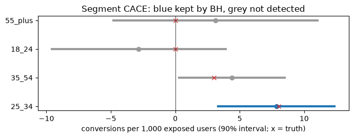

Out [16]:

Segment CACE in conversions per 1,000 exposed users with 90% intervals, truth marked with an x. Only 25 to 34 is kept by Benjamini-Hochberg, at about 8 with an interval from about 3 to 12. The 35 to 54, 18 to 24 and 55 plus intervals are grey (not detected), and the last two cover zero.

8. Class A holdout vs class D platform A/B

Now the CMO’s 18%. The platform split the flight into a creative arm and a house-ad arm, then let its delivery algorithm pick who saw each. It found likelier buyers for the creative arm: a divergent-delivery test. Same true lift, plus a selection gap.

In [17]:

def platform_ab(seed=31, n_per_arm=150_000):          # the platform ran its own split: its own seed
    rng = np.random.default_rng(seed)
    p_a = TRUE["base_cr_reached"]
    p_b = p_a + TRUE["cace_abs_lift"] + TRUE["platform_ab_selection_bias"]   # true lift + who the algorithm picked
    a, b = rng.binomial(n_per_arm, p_a) / n_per_arm, rng.binomial(n_per_arm, p_b) / n_per_arm
    se = np.sqrt(a * (1 - a) / n_per_arm + b * (1 - b) / n_per_arm)
    return 1000 * (b - a), 1000 * se, (b - a) / a


ab, ab_se, ab_rel = platform_ab()
platform = fin.number(ab, (ab - Z90 * ab_se, ab + Z90 * ab_se), cace_e, label="Platform A/B lift (class D)")
print(f"platform relative lift {ab_rel:+.0%}; overstates TRUE CACE by {ab - 1000 * TRUE['cace_abs_lift']:.1f} per 1,000 "
      f"(selection gap {1000 * TRUE['platform_ab_selection_bias']:.1f})")
platform

Out [17]:

platform relative lift +18%; overstates TRUE CACE by 2.6 per 1,000 (selection gap 2.6)

Platform A/B lift (class D): 6.56

likely between 5.39 and 7.73 · medium confidence

details

means	conversions per 1000 exposed users in total, net from removing all spend, exposed, versus the control counterfactual, over 6 weeks, estimator point, 90% confidence
interval	90% confidence 5.39 to 7.73
trust level	2

A tight interval around the wrong number. UMP does not try to argue with it. It classifies it. Both readouts become TestResult documents (plain dicts; the typed form is ump_spec.models.TestResult, and babelfin has no wrapper), then go through fin.check(..., operation="calibrate").

In [18]:

def result(cls, method, number, **extra):
    return {"client_id": "northwind-outdoor", "channel": "youtube", "admissibility_class": cls, "method": method,
            "estimand": cace_e.to_dict(), "lift": number.to_dict(), "outcome": "positive", "duration_weeks": 6,
            "applies_to": {"media_ids": ["youtube"]}, **extra}


doc_a = result("A", "cace", cace, preregistered=True, iroas=iroas.to_dict(), provenance_tier="own-experimental")
doc_d = result("D", "platform_ab", platform, preregistered=False, provenance_tier="platform-reported")
typed = fin.validate("test_result", doc_a)
print(type(typed).__name__, typed.admissibility_class, typed.method)
report_a = fin.check("test_result", doc_a, operation="calibrate")
report_d = fin.check("test_result", doc_d, operation="calibrate")
print("class A:", report_a)
report_d.to_frame()

Out [18]:

TestResult A cace
class A: <GateReport Would pass · 0 stops · 0 fallbacks · 0 warnings · 12 gates (0 fired)>

	gate	outcome	message	codes
0	G-EXP-05	exclude_and_continue	excluded from calibration: ['youtube'] (class D/E or contaminated)	EVIDENCE_EXCLUDED
1	G-EXP-01	fallback	not pre-registered	NOT_PREREGISTERED

The holdout passes clean. The platform A/B is excluded and the flow continues (G-EXP-05, EVIDENCE_EXCLUDED): class D never calibrates incrementality, whatever its interval looks like. The CMO can keep the 18% as a creative signal. It does not go into the model.

9. Attaching to the Tier D MMM: R4 falls back to R6

Northwind’s MMM vendor ships only summary numbers (Tier D). Li asks for route R4 (reweight the posterior). R4 needs joint draws, which a Tier D model does not have.

In [19]:

calibration = {"client_id": "northwind-outdoor", "model_id_in": "mdl_nw_tierD", "route": "R4", "model_tier": "D",
               "tested_channel": "youtube"}
cal_report = fin.check("calibration", calibration, operation="calibrate", context={"test_results": [doc_a]})
cal_report.to_frame()

Out [19]:

	gate	outcome	message	codes
0	G-CAL-02	fallback	no excision chosen: default excision incl. adstock tail applied	DEFAULT_EXCISION
1	G-CAL-04	fallback	Tier D is attach-only; route R4 replaced by R6	ATTACH_ONLY

Both are fallbacks, labelled:

G-CAL-04 ATTACH_ONLY: R4 becomes R6. The readout sits beside the model, and the model is unchanged.
G-CAL-02 DEFAULT_EXCISION: no excision window was chosen, so the default (flight plus adstock tail) applies.

R6 never counts as calibrated. babelfin has no Calibration wrapper, so the typed model answers that directly:

In [20]:

from ump_spec.models import Calibration

attached = Calibration(**{**calibration, "route": "R6", "route_attempted": ["R4", "R6"], "attach_only": True})
print("counts as calibrated:", attached.counts_as_calibrated)

Out [20]:

counts as calibrated: False

10. What Li hands over

Asked: did YouTube drive incremental conversions, and is the platform’s +18% right?
Handed over: the CACE and iROAS below, each with its estimand and 90% interval, checked against the truth.
Assumed or fell back: AOV fixed at $85; the planning prior from the MMM; G-EXP-05 excluded the platform A/B; G-CAL-04 attached the holdout (R6) instead of reweighting; the default excision applied.
Next: recommend the 25 to 34 band; plan a larger follow-up for 35 to 54 (“not detected” there means underpowered); ask the MMM vendor for Tier B curves so a later readout can actually calibrate.

In [21]:

handover = [itt, cace, iroas]
check = pd.DataFrame({"number": [n.label for n in handover], "value": [n.value for n in handover],
                      "lo": [n.lo for n in handover], "hi": [n.hi for n in handover],
                      "truth": [1000 * TRUE["itt_abs_lift"], 1000 * TRUE["cace_abs_lift"], TRUE["iroas"]]})
check["covered"] = (check.lo <= check.truth) & (check.truth <= check.hi)
print(f"CACE / ITT = {cace.value / itt.value:.2f} (1 / reach = {1 / est['reach']:.2f})")
check.round(2)

Out [21]:

CACE / ITT = 2.86 (1 / reach = 2.86)

	number	value	lo	hi	truth	covered
0	YouTube ITT lift	1.53	0.62	2.45	1.40	True
1	YouTube CACE lift	4.39	1.77	7.00	4.00	True
2	YouTube iROAS	1.74	0.70	2.78	1.59	True

Going deeper

Spec §9 (test plans and admissibility classes A to E) and §10 (calibration routes R1 to R6, BH conflicts).
docs/06-mmm-ema-technical-guide.md: EIG/EVOI, power and non-geo RCTs.
Notebook 01 for fin.compare and the alignment ladder; notebook 02 for fin.check and gate reports.

Next: take the same readout to a Tier B model, where R5 can adjust the YouTube curve instead of attaching.